---
title: "A Statistical Primer"
---
```{=latex}
\mainmatter
```
```{python}
#| label: python-setup-03-statistical-primer
#| include: false
import numpy as np
import pandas as pd
import matplotlib.pyplot as plt
import seaborn as sns
from scipy import stats
```
## Learning Objectives
::: {.callout-note icon="false"}
## 📘 What You'll Learn in This Chapter
By the end of this chapter, you will be able to:
- Distinguish between populations and samples, understand why we sample, and recognize sampling bias
- Compute and interpret measures of central tendency: mean (arithmetic, weighted, geometric, harmonic), median, and mode
- Explain how skewness affects the relationship between mean and median, and when to use each
- Calculate and interpret measures of spread: range, variance, standard deviation, interquartile range (IQR), and coefficient of variation
- Understand the intuition behind variance, variance as a squared quantity, and why this matters
- Define probability formally using classical, frequentist, and subjective definitions
- Apply probability rules: addition, multiplication, complement, and conditional probability
- Understand and apply Bayes' theorem in practical contexts
- Work with discrete probability distributions (Bernoulli, Binomial, Poisson) and continuous distributions (Uniform, Normal, Exponential)
- Recognize and explain the Central Limit Theorem—the most important result in statistics
- Construct confidence intervals and interpret them correctly
- Understand the t-distribution and its role in small samples
:::
---
## Populations and Samples: Why We Sample and How Sampling Works
Imagine you're a market researcher in Nigeria tasked with understanding the financial behavior of Nigerian adults. The **population** you care about is roughly 90 million adults. Ideally, you'd collect data on all 90 million—their income, spending, savings, debt—and compute exact statistics about them.
But this is impossible. You can't interview 90 million people. You can't afford it; you don't have time; it's logistically infeasible.
This is why we sample. A **sample** is a subset of the population, selected strategically. We collect data from, say, 2,000 Nigerians and use their data to estimate what's true about all 90 million.
**Population:** The entire group we care about
**Sample:** A subset we actually measure
**Parameter:** A true characteristic of the population (usually unknown)
**Statistic:** A measured characteristic of the sample (what we compute)
For example:
- Population parameter: "The true average monthly income of Nigerian adults" (unknown; we can't measure 90 million people)
- Sample statistic: "The average monthly income of our 2,000 sampled Nigerians: ₦85,000" (what we observe)
The sample statistic is our *estimate* of the population parameter. It's rarely exactly right, but if we sample carefully, it's close.
### Why Sample Rather Than Census?
A **census** is an attempt to measure the entire population. Nigeria conducts a national census every 10 years. But censuses are expensive, time-consuming, and prone to error. For business analytics, we sample because:
1. **Cost:** Sampling 2,000 people costs far less than surveying 2,000,000
2. **Speed:** You can get results in weeks instead of months or years
3. **Feasibility:** Some measurements are destructive (testing the lifespan of a battery means running it until it dies) and you can't do this to every unit
4. **Practical value:** A 95% accurate estimate in 2 weeks is more useful than a 99% accurate census result in 6 months
The trade-off: sampling introduces **sampling error**—random variation in the sample statistic due to which particular observations we happened to include.
### Sampling Bias: The Danger
The critical challenge is **sampling bias**: systematically collecting a sample that doesn't represent the population.
::: {.callout-caution icon="false"}
## 📝 Review Questions: Populations and Samples
1. A bank wants to understand its customer base's average annual income. The population is 500,000 customers. Why is sampling preferable to measuring every customer?
2. A survey is conducted online on a bank's website, asking customers about their satisfaction. Is this sampling method likely to have bias? Explain. Who is missing from this sample?
3. The National Bureau of Statistics conducts a household survey to estimate employment rates across Nigeria. Would a sample of households in Lagos alone represent the entire population of Nigeria? Why or why not?
:::
### Sampling Methods
To reduce bias, researchers use formal sampling methods. Here are the main ones:
**Simple Random Sampling:** Every member of the population has an equal chance of being selected. You create a numbered list of the population (1 to 500,000 for your bank customers) and randomly select 2,000 numbers. This is the gold standard—it's unbiased, but it requires a complete list of the population.
**Stratified Random Sampling:** Divide the population into strata (groups) and sample randomly from within each stratum. For a bank, you might divide customers by account type (Savings, Checking, Business) and sample within each type proportionally. If 50% of customers are Savings, 50% of your sample will be Savings. This ensures representation of each segment and often reduces sampling error.
**Cluster Sampling:** Divide the population into clusters (geographic regions, branches) and randomly select clusters. If you're sampling a bank's customers, you might randomly select 10 branches and survey all customers from those branches. This is cheaper and faster than simple random sampling but more prone to bias if clusters differ from each other.
**Systematic Sampling:** Select every kth observation from an ordered list. If your population has 500,000 customers, divide by desired sample size (2,000) to get k = 250. Start at a random number between 1 and 250, then select every 250th customer thereafter. Fast and practical but can introduce bias if the list has hidden patterns.
### Sampling Bias: Nigerian Examples
**Example 1 - Urban Bias:** A telecommunications company surveys customer satisfaction online. The sample is biased toward customers who use the company's internet service regularly (since they're taking the survey online). Rural customers without reliable broadband are underrepresented. **Bias:** The sample overrepresents satisfied digital-native customers and underrepresents others.
**Example 2 - Self-Selection Bias:** A bank sends a survey link to customers, asking about recent credit card experience. Only customers with strong feelings (very satisfied or very upset) are likely to respond. **Bias:** The sample is weighted toward extreme opinions; moderate, satisfied customers don't bother responding. The estimated satisfaction will be polarized and unrepresentative.
**Example 3 - Time-of-Day Bias:** A retailer in Lagos conducts street surveys of mall shoppers. Surveys happen 10 AM - 4 PM on weekdays. **Bias:** Working professionals and students are underrepresented; retirees and shift workers are overrepresented. The sample doesn't represent the general population's preferences.
The antidote to sampling bias is **random selection** with no systematic pattern that favors some population members over others.
---
## Measures of Central Tendency: Finding the Middle
A sample of 2,000 Nigerian adults contains 2,000 income values. You need a single number to represent "the typical income." This is a **measure of central tendency**—a value that represents the center of the data.
Three measures are in common use: **mean**, **median**, and **mode**. Each tells a different story.
### The Arithmetic Mean
The **mean** (or average) is the sum of all values divided by the count. If your sample has incomes: ₦50k, ₦75k, ₦80k, ₦100k, ₦500k, the mean is (50 + 75 + 80 + 100 + 500) / 5 = 161k.
::: {.callout-tip icon="false"}
## 🔑 Arithmetic Mean Formula
$$\bar{x} = \frac{1}{n} \sum_{i=1}^{n} x_i = \frac{x_1 + x_2 + \ldots + x_n}{n}$$
Where:
- $\bar{x}$ is the sample mean
- $x_i$ is the value of the *i*-th observation
- $n$ is the number of observations
:::
The mean is intuitive and has nice mathematical properties (it's at the heart of many statistical methods). But it's sensitive to outliers. In the example above, one high income (₦500k) pulls the mean way up. Most people earn ₦50k-₦100k, but the mean says ₦161k—unrepresentative.
**Why the mean has this flaw:** The mean is calculated using every single value, including extreme outliers. A few very rich Nigerians pull the mean of "typical income" far above what most people actually earn.
### The Median
The **median** is the middle value when data is sorted. In the income example, sorted: ₦50k, ₦75k, ₦80k, ₦100k, ₦500k. The median is ₦80k—the 3rd of 5 values. Half earn more; half earn less.
For an even number of observations, the median is the average of the two middle values.
The median is robust to outliers. Whether the highest income is ₦500k or ₦5 million, the median stays ₦80k. This makes it a better representation of "typical" when outliers exist.
**When to use median:** Use the median when you care about "typical" and your data has outliers. Income, house prices, and other economic data often have outliers, so median is often preferred for these.
### The Mode
The **mode** is the most frequent value. In a survey of account types (Savings, Checking, Business, Student), if 40% of customers have Savings accounts, the mode is "Savings."
The mode is the only measure of central tendency that works for categorical data.
### Skewness: How Outliers Affect the Mean vs. Median
**Skewness** measures whether a distribution is lopsided. A distribution can be:
- **Symmetric:** Mean = Median. Outliers are balanced on both sides.
- **Right-skewed (positively skewed):** Long tail on the right (high values). Mean > Median. Examples: income, company size (few very large companies pull the mean up). This is the common pattern in Nigerian economic data.
- **Left-skewed (negatively skewed):** Long tail on the left (low values). Mean < Median. Example: test scores on an easy exam (few low scores pull the mean down).
::: {.callout-tip icon="false"}
## 🔑 The Right-Skewed Distribution (Common in Economics)
Imagine Nigerian household incomes:
- Most people earn ₦100k - ₦500k monthly
- A smaller group earns ₦500k - ₦2M
- A tiny group earns ₦2M+
The few very rich households have high incomes that pull the mean far above the median. The mean might be ₦750k (artificially high) while the median is ₦300k (what most people actually earn).
:::
This matters for decision-making. A bank using mean income would overestimate typical customers' earning power. A politician using median income would get closer to reality.
### Weighted Mean
Sometimes observations have different importance. A **weighted mean** assigns weights to each value.
::: {.callout-tip icon="false"}
## 🔑 Weighted Mean Formula
$$\bar{x}_w = \frac{\sum_{i=1}^{n} w_i x_i}{\sum_{i=1}^{n} w_i}$$
Where $w_i$ is the weight of observation $i$.
:::
**Example:** A portfolio has three stocks: ₦1M in Stock A (return 10%), ₦2M in Stock B (return 15%), ₦3M in Stock C (return 8%). The weighted average return is:
$$\bar{r} = \frac{(1M \times 0.10) + (2M \times 0.15) + (3M \times 0.08)}{1M + 2M + 3M} = \frac{0.1M + 0.3M + 0.24M}{6M} = \frac{0.64M}{6M} = 0.1067 = 10.67\%$$
This is more accurate than the simple average (10 + 15 + 8) / 3 = 11%, which ignores that you have more money in lower-return Stock C.
### Geometric Mean
The **geometric mean** is used for growth rates and percentages. If an investment grows 10% one year, then 20% the next, the average growth is not (10 + 20) / 2 = 15%. It's the geometric mean.
::: {.callout-tip icon="false"}
## 🔑 Geometric Mean Formula
$$\bar{x}_g = \sqrt[n]{x_1 \times x_2 \times \ldots \times x_n}$$
Or, for growth rates: multiply the growth factors, then take the nth root.
:::
If an investment is worth ₦100 in year 0, grows to ₦110 (10% growth) in year 1, then to ₦132 (20% growth) in year 2:
Growth factors: 1.10, 1.20
Geometric mean of growth factors: $\sqrt{1.10 \times 1.20} = \sqrt{1.32} = 1.149$
Average annual growth rate: 14.9%
Check: ₦100 × 1.149 = ₦114.9 (year 1), then ₦114.9 × 1.149 = ₦132 (year 2). Correct!
### Harmonic Mean
The **harmonic mean** is used for rates and ratios. If a car travels from Lagos to Abuja (200 km) at 80 km/hr, then returns at 100 km/hr, what's the average speed?
The simple mean would be (80 + 100) / 2 = 90 km/hr, but this is wrong. The car spends more time going at 80 km/hr (slower), so the average should be less than 90.
::: {.callout-tip icon="false"}
## 🔑 Harmonic Mean Formula
$$\bar{x}_h = \frac{n}{\frac{1}{x_1} + \frac{1}{x_2} + \ldots + \frac{1}{x_n}}$$
:::
$$\bar{x}_h = \frac{2}{\frac{1}{80} + \frac{1}{100}} = \frac{2}{0.0125 + 0.0100} = \frac{2}{0.0225} = 88.9 \text{ km/hr}$$
Check: 200 km at 80 km/hr = 2.5 hours; 200 km at 100 km/hr = 2 hours. Total: 400 km in 4.5 hours = 88.9 km/hr. Correct!
---
## Section Review: Central Tendency and Skewness
::: {.callout-caution icon="false"}
## 📝 Review Questions: Measures of Central Tendency
1. A bank has 10,000 customers. Nine thousand earn between ₦200k and ₦500k monthly. One thousand earn between ₦5M and ₦50M monthly. Would the mean or median better represent "typical customer income"? Why?
2. Compute the mean, median, and mode for the following incomes (in thousands): 30, 35, 40, 40, 45, 50, 200. Explain the difference between the mean and median and what this suggests about the distribution.
3. An investment grows 20% in year 1 and 10% in year 2. Is the average growth rate 15%? Why or why not? What is the correct average growth rate?
4. A company has three divisions with average salaries: Division A, 100 employees at ₦500k average; Division B, 200 employees at ₦600k average; Division C, 50 employees at ₦800k average. What is the overall company average salary? (Hint: use weighted mean.)
5. In a right-skewed distribution (e.g., household income), why is mean > median? Draw a rough sketch showing this relationship.
:::
---
## Measures of Spread: How Dispersed Is the Data?
Imagine two bank branches, each serving 100 customers with daily transaction volumes:
- **Branch A:** Consistent: Every day, 80-120 transactions (around 100)
- **Branch B:** Volatile: Some days 50 transactions, some days 150 (average 100)
Both branches average 100 transactions, but they're very different. Branch A's operations are predictable; Branch B's are chaotic. Measures of **spread** (or **dispersion**) quantify this variability.
### Range
The **range** is the simplest measure: maximum value minus minimum value.
- Branch A: 120 - 80 = 40 transactions
- Branch B: 150 - 50 = 100 transactions
Range is intuitive but crude. A single extreme outlier can inflate it artificially.
### Variance and Standard Deviation
**Variance** measures the average squared distance from the mean. Why squared? To penalize large deviations more than small ones and to eliminate the sign (distance is always positive).
::: {.callout-tip icon="false"}
## 🔑 Variance and Standard Deviation
$$s^2 = \frac{1}{n-1} \sum_{i=1}^{n} (x_i - \bar{x})^2$$
$$s = \sqrt{s^2}$$
Where:
- $s^2$ is the sample variance
- $s$ is the sample standard deviation
- $(x_i - \bar{x})$ is the deviation of observation $i$ from the mean
- We divide by $n-1$ (not $n$) for technical reasons: this makes $s^2$ an unbiased estimator of the true population variance
:::
**The key insight:** Variance is in squared units. If you're measuring income in Naira, variance is in Naira². This is why standard deviation—the square root of variance, in the original units—is often easier to interpret.
**Example:**
Data: 80, 90, 100, 110, 120 transactions
Mean: 100
Deviations: -20, -10, 0, 10, 20
Squared deviations: 400, 100, 0, 100, 400
Variance: (400 + 100 + 0 + 100 + 400) / 4 = 250 (note: dividing by n-1 = 4, not n = 5)
Standard deviation: √250 = 15.8 transactions
Interpretation: Observations typically deviate from the mean by about 15.8 transactions.
### Interquartile Range (IQR)
The **interquartile range** is the difference between the 75th percentile (Q3) and 25th percentile (Q1).
For the transaction data (80, 90, 100, 110, 120):
- Q1 (25th percentile): 90
- Q3 (75th percentile): 110
- IQR: 110 - 90 = 20
IQR captures the spread of the middle 50% of data, ignoring outliers. It's robust and often used in box plots.
### Coefficient of Variation
The **coefficient of variation (CV)** is the standard deviation divided by the mean. It's unitless and lets you compare spread across variables with different scales.
::: {.callout-tip icon="false"}
## 🔑 Coefficient of Variation
$$CV = \frac{s}{\bar{x}} \times 100\%$$
:::
**Example:**
Branch A: mean 100, std dev 15.8, CV = 15.8%
Branch B: mean 100, std dev 30, CV = 30%
Branch B is more variable (30% variation) than Branch A (15% variation).
**Use CV when:** Comparing variables with different units or scales. For instance, comparing volatility of stock prices (₦1,000 to ₦10,000 range) to volatility of cryptocurrency (₦100 to ₦1,000,000 range) requires CV, not just standard deviation.
---
## Section Review: Measures of Spread
::: {.callout-caution icon="false"}
## 📝 Review Questions: Measures of Spread
1. Two investment funds have average annual returns of 12%. Fund A's standard deviation is 5%; Fund B's is 15%. Which is riskier, and why would an investor care about this difference?
2. Why is variance in squared units (e.g., Naira²) unnatural to interpret, and what solution do we use?
3. A bank wants to compare the variability of customer wait times (hours) across two branches. Branch A: mean 0.5 hours, std dev 0.1 hours. Branch B: mean 2 hours, std dev 0.3 hours. Which has higher relative variability? (Use coefficient of variation.)
4. Data: 10, 15, 20, 25, 30. Compute the mean, standard deviation, and range. If you removed the value 30, how would each measure change?
5. Why is the interquartile range (IQR) often preferred over range when data has outliers?
:::
---
## Probability Fundamentals: The Language of Uncertainty
Statistics is about making decisions under uncertainty. **Probability** is the language we use to quantify uncertainty.
What does it mean to say "There's a 30% probability it will rain tomorrow"? Different interpretations exist:
### Classical Probability
The **classical definition** applies when outcomes are equally likely. The probability of an event is:
$$P(A) = \frac{\text{Number of outcomes favoring A}}{\text{Total number of equally likely outcomes}}$$
**Example:** A fair die has six equally likely faces. The probability of rolling a 3 is 1/6 ≈ 0.167.
The classical definition works for gambling and formal games but doesn't apply well to real-world events (like rain tomorrow—the outcomes aren't equally likely).
### Frequentist Probability
The **frequentist definition** bases probability on long-run frequency: if you repeat an experiment infinitely many times, the probability is the limiting proportion of successes.
$$P(A) = \lim_{n \to \infty} \frac{\text{Number of times A occurs}}{n}$$
**Example:** To estimate the probability that a Nigerian bank customer defaults on a loan, look at historical data: "Of 100,000 loans issued, 8,000 defaulted. P(default) ≈ 0.08 = 8%."
This is the definition most useful for analytics. Historical data gives us observed frequencies, which we treat as probability estimates.
### Subjective Probability
The **subjective definition** treats probability as personal belief or credibility, updated as you learn.
**Example:** "I think there's a 70% chance our startup will secure Series A funding next year."
This captures expert judgment. Bayesian statistics formalizes subjective probability, allowing you to update beliefs as you gather data.
---
### Basic Probability Rules
**Rule 1: Probabilities are between 0 and 1**
An impossible event has probability 0. A certain event has probability 1. Everything else is in between.
$$0 \leq P(A) \leq 1$$
**Rule 2: Complement Rule**
The probability of an event not occurring is 1 minus the probability it does occur.
$$P(\text{not } A) = 1 - P(A)$$
If P(customer buys) = 0.3, then P(customer doesn't buy) = 0.7.
**Rule 3: Addition Rule**
For two events A and B:
$$P(A \text{ or } B) = P(A) + P(B) - P(A \text{ and } B)$$
We subtract $P(A \text{ and } B)$ to avoid double-counting cases where both occur.
**Example:** At a bank, 40% of customers have a savings account (S), 30% have a checking account (C), 20% have both.
$$P(S \text{ or } C) = 0.40 + 0.30 - 0.20 = 0.50$$
50% of customers have at least one account.
**Rule 4: Multiplication Rule**
For two independent events (where one doesn't affect the other):
$$P(A \text{ and } B) = P(A) \times P(B)$$
**Example:** A customer applies for two loans independently. P(approval for loan 1) = 0.8, P(approval for loan 2) = 0.7.
$$P(\text{approved for both}) = 0.8 \times 0.7 = 0.56$$
---
### Conditional Probability
**Conditional probability** is the probability of an event given that another event has occurred. We write $P(A | B)$, read as "probability of A given B."
$$P(A | B) = \frac{P(A \text{ and } B)}{P(B)}$$
**Example:** A bank observes:
- 5% of customers are students (S)
- 15% of customers have defaulted (D)
- 1% of customers are both students and have defaulted
What's the probability that a customer defaulted, *given that they're a student*?
$$P(D | S) = \frac{P(D \text{ and } S)}{P(S)} = \frac{0.01}{0.05} = 0.20 = 20\%$$
Students default at a 20% rate, compared to the overall 15% rate. Students are higher risk.
---
### Bayes' Theorem: Updating Beliefs With Data
**Bayes' Theorem** is the workhorse of probability. It tells us how to update our beliefs when we observe new evidence.
::: {.callout-tip icon="false"}
## 🔑 Bayes' Theorem
$$P(A | B) = \frac{P(B | A) \times P(A)}{P(B)}$$
Where:
- $P(A | B)$ is the **posterior** probability (updated belief after seeing evidence B)
- $P(B | A)$ is the **likelihood** (probability of observing B if A is true)
- $P(A)$ is the **prior** probability (belief before seeing evidence B)
- $P(B)$ is the **marginal likelihood** (probability of observing B overall)
:::
**Intuitive interpretation:** Start with a prior belief $P(A)$. Observe evidence $B$. Update your belief using the likelihood $P(B | A)$ to get posterior $P(A | B)$.
**Example (Medical Testing):** A test for a disease has 99% accuracy:
- If you have the disease, the test is positive 99% of the time: $P(\text{positive} | \text{disease}) = 0.99$
- If you don't have the disease, the test is negative 99% of the time: $P(\text{negative} | \text{no disease}) = 0.99$
The disease is rare: 1 in 10,000 people have it: $P(\text{disease}) = 0.0001$
You test positive. What's the probability you actually have the disease?
$$P(\text{disease} | \text{positive}) = \frac{P(\text{positive} | \text{disease}) \times P(\text{disease})}{P(\text{positive})}$$
We need $P(\text{positive})$:
$$P(\text{positive}) = P(\text{positive} | \text{disease}) \times P(\text{disease}) + P(\text{positive} | \text{no disease}) \times P(\text{no disease})$$
$$= 0.99 \times 0.0001 + 0.01 \times 0.9999 = 0.000099 + 0.009999 = 0.010098$$
$$P(\text{disease} | \text{positive}) = \frac{0.99 \times 0.0001}{0.010098} = \frac{0.000099}{0.010098} \approx 0.0098 = 0.98\%$$
**Key insight:** Even though the test is 99% accurate, a positive result only gives you a 0.98% chance of having the disease. Why? Because the disease is so rare that false positives (1% of the 99.99% healthy people) outnumber true positives.
This is Bayes' theorem in action: updating a very low prior (0.01%) with evidence that's not perfectly informative (99% accurate) gives a still-low posterior (0.98%).
---
## Section Review: Probability
::: {.callout-caution icon="false"}
## 📝 Review Questions: Probability Fundamentals
1. Define probability in three different ways (classical, frequentist, subjective). Give an example where each definition is most appropriate.
2. A bank has 1,000 customers. 400 have a savings account, 300 have a credit card, 100 have both. What's the probability a random customer has a savings account OR a credit card?
3. Among loan applicants, 40% are employed and 60% are unemployed. Of employed applicants, 90% are approved. Of unemployed, 40% are approved. What's the probability a randomly chosen applicant is approved? (Use the law of total probability.)
4. A fraud detection system catches 95% of fraudulent transactions but has a 1% false positive rate. If 0.1% of transactions are actually fraudulent, what's the probability that a flagged transaction is actually fraudulent? (Use Bayes' theorem.)
5. Explain why $P(A \text{ and } B) = P(A) \times P(B)$ only holds when A and B are independent.
:::
---
## Probability Distributions: Models of Randomness
A **probability distribution** is a mathematical model that describes the probabilities of different outcomes for a random variable.
Imagine flipping a coin 100 times and recording heads (1) or tails (0). The outcomes vary randomly, but follow a pattern. A distribution captures that pattern.
Distributions come in two types: **discrete** (countable outcomes: 0, 1, 2, 3...) and **continuous** (infinite outcomes: any real number).
### Discrete Distributions
#### The Bernoulli Distribution
The **Bernoulli distribution** models a single trial with two outcomes: success (1) or failure (0), each with probability $p$.
$$P(X = 1) = p, \quad P(X = 0) = 1 - p$$
**Business examples:**
- A customer either buys (1) or doesn't (0)
- A loan applicant is approved (1) or rejected (0)
- A transaction is fraudulent (1) or legitimate (0)
If you know the probability $p$ of the outcome, you know the Bernoulli distribution completely.
#### The Binomial Distribution
The **Binomial distribution** models the number of successes in $n$ independent Bernoulli trials.
::: {.callout-tip icon="false"}
## 🔑 Binomial Distribution
If $X$ is the number of successes in $n$ independent trials, each with success probability $p$:
$$P(X = k) = \binom{n}{k} p^k (1-p)^{n-k}$$
Where $\binom{n}{k} = \frac{n!}{k!(n-k)!}$ is the binomial coefficient.
The mean is $\mu = np$ and the variance is $\sigma^2 = np(1-p)$.
:::
**Example:** A loan portfolio has 100 loans, each with 5% default probability. What's the probability that exactly 3 loans default?
$$P(X = 3) = \binom{100}{3} (0.05)^3 (0.95)^{97}$$
This calculation is complex by hand but easy in software (R or Python).
**Business applications:**
- Quality control: Of 1,000 units produced, how many are defective?
- Marketing: Of 500 emails sent, how many result in a click?
- Lending: Of 1,000 loans, how many will default?
#### The Poisson Distribution
The **Poisson distribution** models the number of rare events occurring in a fixed time period or region.
::: {.callout-tip icon="false"}
## 🔑 Poisson Distribution
If $X$ is the number of events in a fixed period, with average rate $\lambda$:
$$P(X = k) = \frac{e^{-\lambda} \lambda^k}{k!}$$
Where $e \approx 2.718$. The mean is $\mu = \lambda$ and the variance is $\sigma^2 = \lambda$.
:::
**Example:** A bank's fraud detection system flags an average of 5 transactions per day as suspicious. What's the probability of exactly 8 flagged transactions tomorrow?
$$P(X = 8) = \frac{e^{-5} \times 5^8}{8!} \approx 0.065 = 6.5\%$$
**Business applications:**
- Number of customer service calls per hour (with known average rate)
- Number of equipment failures per year
- Number of defects in a batch of products
- Frequency of rare events like system outages or data breaches
### Continuous Distributions
#### The Uniform Distribution
All values in a range are equally likely. If $X$ is uniform on [a, b]:
$$P(a \leq X \leq b) = 1, \quad P(X = c) = \frac{1}{b-a}$$
**Example:** A customer's arrival time at a store is equally likely anywhere between 9 AM and 5 PM. This is uniform on [9, 17] hours.
#### The Normal (Gaussian) Distribution
The **normal distribution** is the most important distribution in statistics. It appears everywhere: heights, test scores, errors in measurements, IQ scores. Many phenomena in nature and business follow this pattern.
::: {.callout-tip icon="false"}
## 🔑 Normal Distribution
A normal distribution is determined by two parameters: mean $\mu$ and standard deviation $\sigma$.
The probability density function is:
$$f(x) = \frac{1}{\sigma \sqrt{2\pi}} e^{-\frac{(x-\mu)^2}{2\sigma^2}}$$
The distribution is symmetric and bell-shaped, with most values near the mean and fewer far away.
The **68-95-99.7 rule:** Approximately 68% of data falls within 1 standard deviation of the mean, 95% within 2, and 99.7% within 3.
:::
**Why the normal distribution is important:**
1. **It appears everywhere:** Many quantities in nature and business are approximately normal
2. **Central Limit Theorem:** The average of any distribution approaches normal as sample size grows
3. **Simplicity:** It's easy to work with mathematically
4. **Statistical tests:** Most common statistical tests assume normality
**Nigerian examples:**
- Distribution of customer incomes (approximately normal, though often right-skewed)
- Distribution of product weights from a factory (approximately normal if production is stable)
- Distribution of test scores across students (approximately normal if the test is well-designed)
#### The Exponential Distribution
The **exponential distribution** models the time between rare events (like equipment failures or customer arrivals).
**Example:** Customer arrivals at a store follow a Poisson distribution with an average of 10 per hour. The time between arrivals follows an exponential distribution with mean 1/10 hour = 6 minutes.
---
## Section Review: Probability Distributions
::: {.callout-caution icon="false"}
## 📝 Review Questions: Probability Distributions
1. A loan officer approves 80% of applications. Is this a Bernoulli or Binomial process? If they review 25 applications, what distribution models the number of approvals?
2. An email marketing campaign has a click-through rate of 2%. You send 5,000 emails. Is this a Bernoulli or Binomial distribution? What are the expected number of clicks and the standard deviation?
3. A customer service call center receives an average of 15 calls per hour. Why is the Poisson distribution appropriate here? What's the probability of exactly 20 calls in the next hour?
4. Test scores at a Nigerian university are approximately normal with mean 65 and standard deviation 10. What percentage of students score between 45 and 85? (Use the 68-95-99.7 rule.)
5. Why is the normal distribution so important in statistics, even if most real data isn't perfectly normal?
:::
---
## The Central Limit Theorem: The Most Important Result in Statistics
The **Central Limit Theorem (CLT)** is the bedrock of modern statistics. It's the reason we can make inferences about populations from samples, even when we don't know the population distribution.
### The Theorem
Imagine a population with some distribution (any distribution—normal, skewed, uniform, anything). You repeatedly sample $n$ observations from this population and compute the sample mean $\bar{x}$ for each sample. You collect many sample means and look at their distribution.
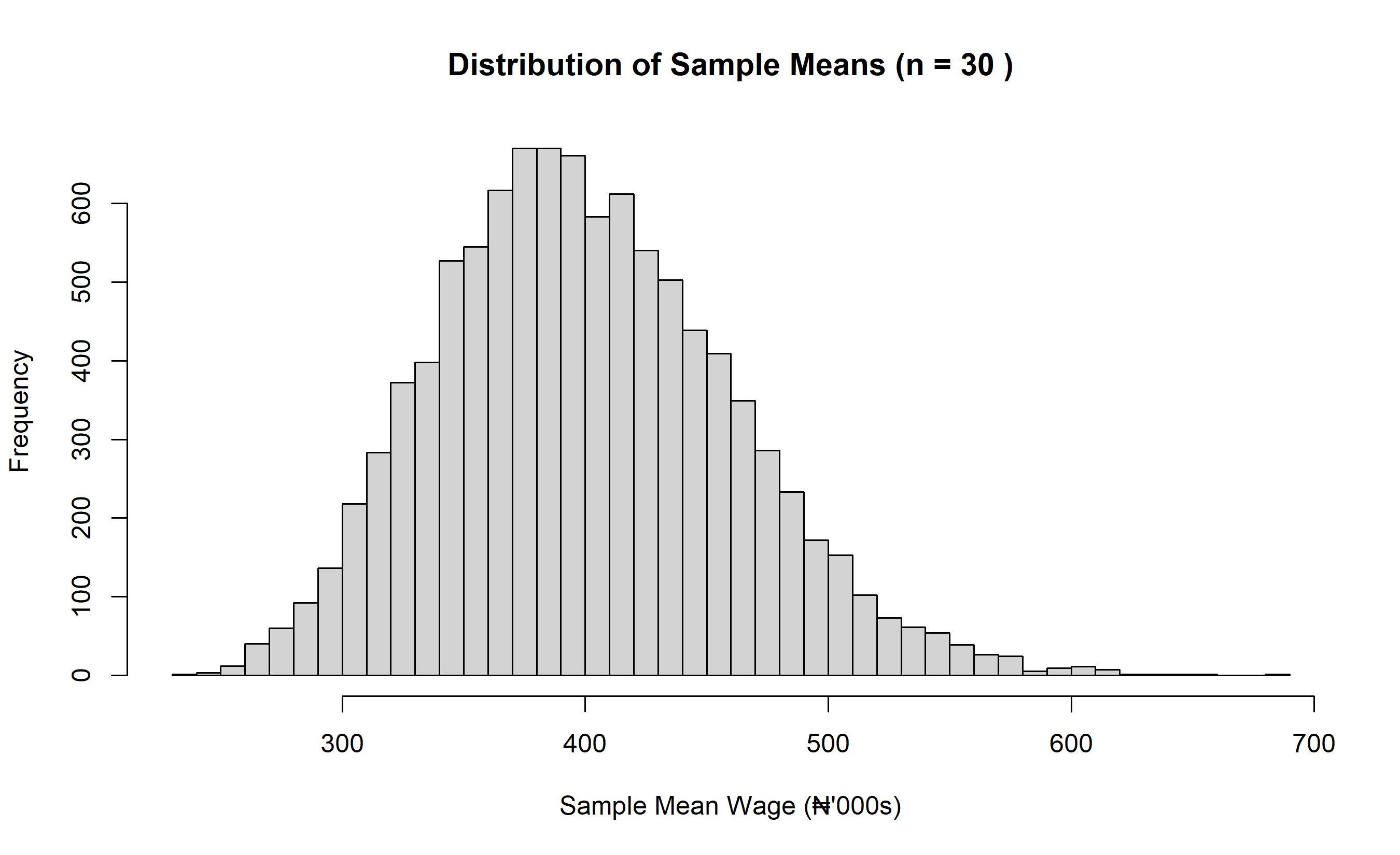
The Central Limit Theorem says: **As $n$ gets larger, the distribution of sample means becomes approximately normal, regardless of the population distribution.**
This is stunning. The population might be skewed, bimodal, anything. But the distribution of sample means becomes normal.
### Why This Matters
This gives us enormous power:
1. We can use normal distribution properties (like the 68-95-99.7 rule) for any population
2. We can construct confidence intervals and hypothesis tests
3. We can make inferences from samples even when we don't know the population exactly
### Understanding CLT Through Simulation
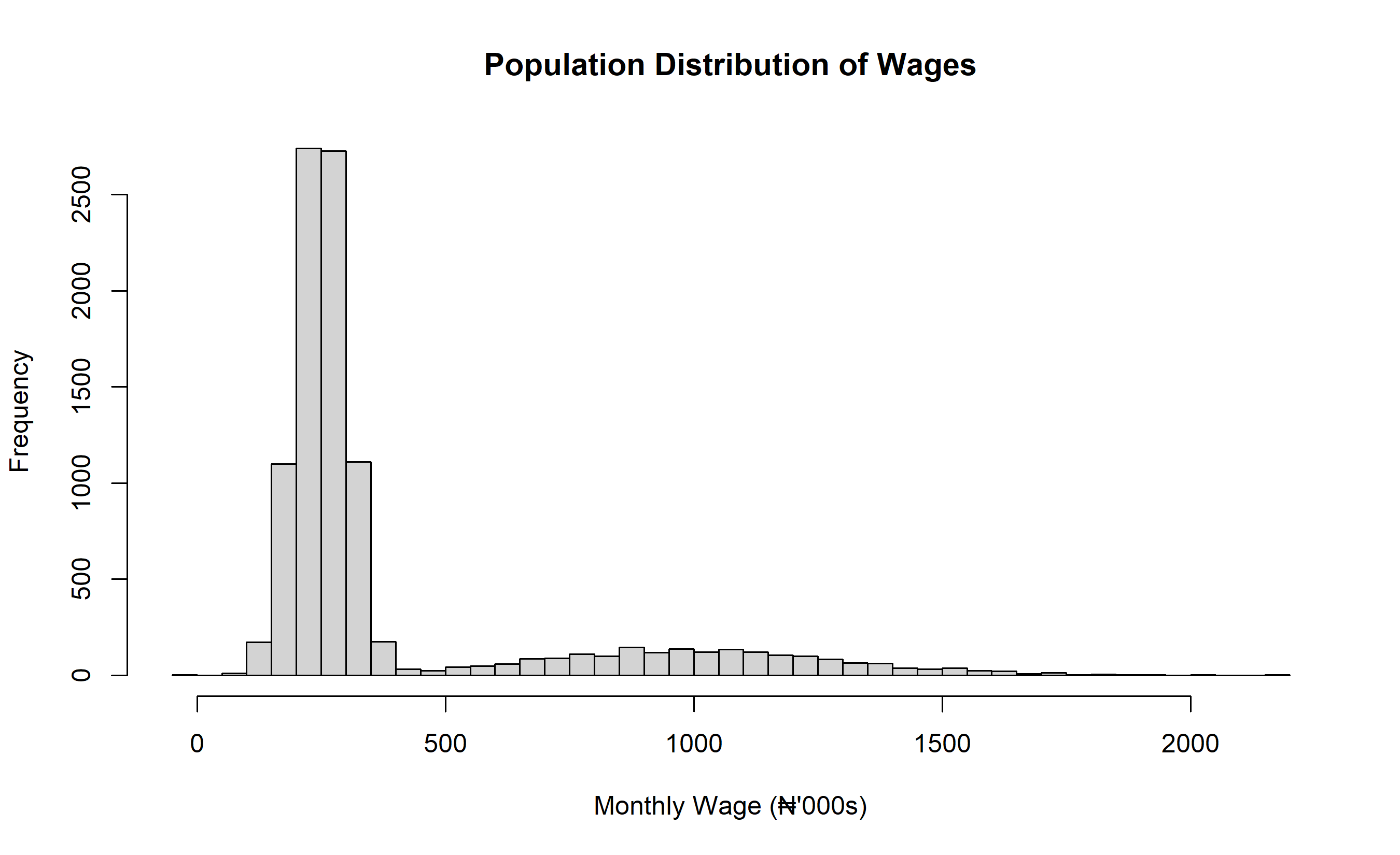
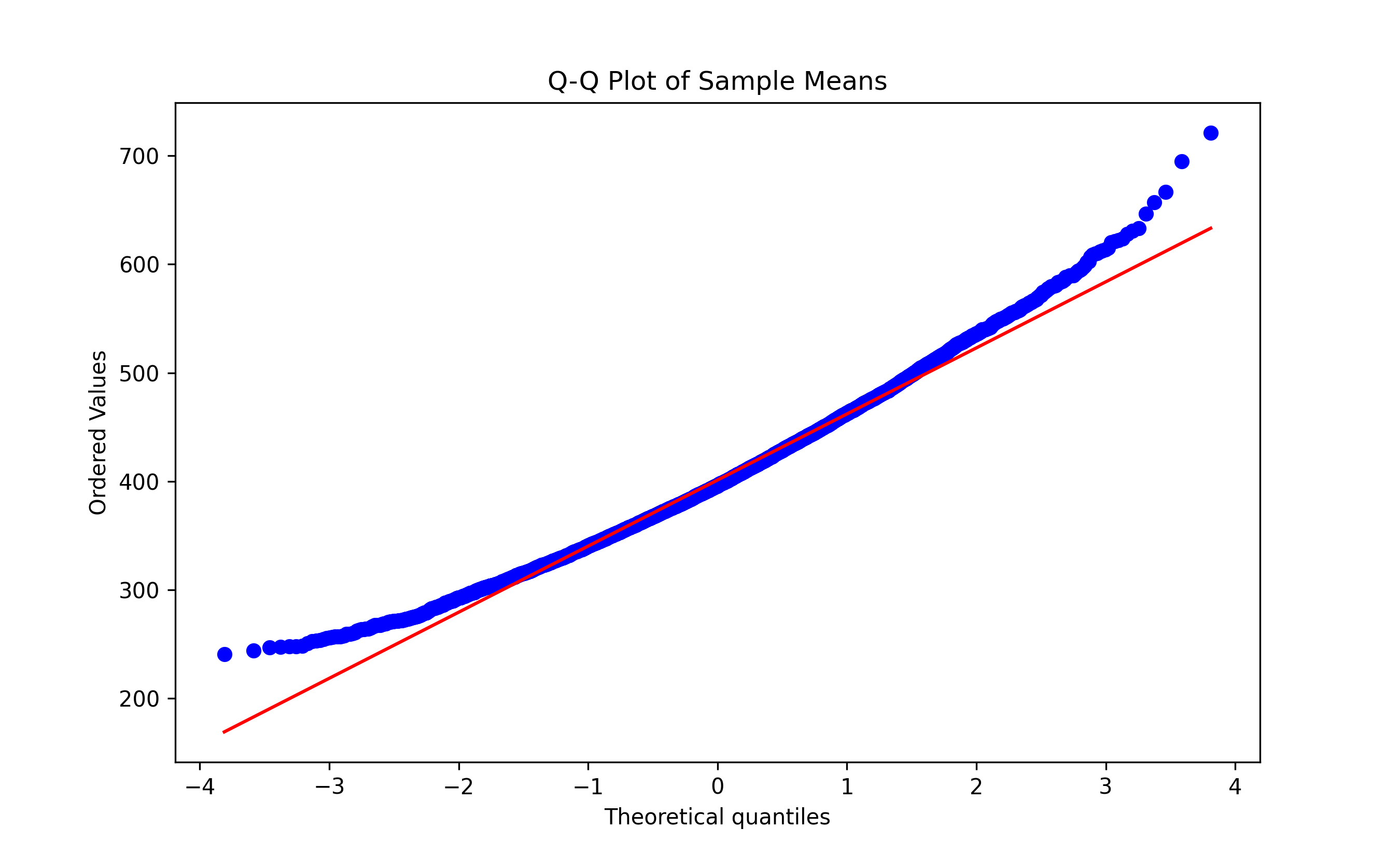
Let's see this in action with data from a Nigerian wage survey. Suppose the true population distribution of monthly wages is bimodal (right-skewed: many people earning ₦200k-₦300k, and a smaller group earning ₦500k-₦2M). This is not normal; it's distinctly non-normal.
Now we simulate the CLT:
::: {.panel-tabset}
## R
```{r}
# Simulate bimodal population of wages (in thousands Naira)
set.seed(123)
population <- c(
  rnorm(8000, mean = 250, sd = 50),  # 8000 people earning ~250k
  rnorm(2000, mean = 1000, sd = 300) # 2000 people earning ~1M
)

# Visualize population distribution
hist(population, breaks = 50,
     main = "Population Distribution of Wages",
     xlab = "Monthly Wage (₦'000s)")
# Now simulate sampling: take many samples of size n=30
sample_size <- 30
num_samples <- 10000
sample_means <- replicate(num_samples, mean(sample(population, sample_size)))

# Visualize distribution of sample means
hist(sample_means, breaks = 50,
     main = paste("Distribution of Sample Means (n =", sample_size, ")"),
     xlab = "Sample Mean Wage (₦'000s)")
# The sample means are approximately normal!
# Check with a Q-Q plot
qqnorm(sample_means)
qqline(sample_means)
```
## Python
```{python}
import numpy as np
import matplotlib.pyplot as plt
from scipy import stats

# Simulate bimodal population
np.random.seed(123)
pop1 = np.random.normal(loc=250, scale=50, size=8000)
pop2 = np.random.normal(loc=1000, scale=300, size=2000)
population = np.concatenate([pop1, pop2])

# Visualize population
plt.figure(figsize=(12, 4))
plt.subplot(1, 2, 1)
plt.hist(population, bins=50, edgecolor='black')
plt.title("Population Distribution of Wages")
plt.xlabel("Monthly Wage (₦'000s)")
plt.ylabel("Frequency")

# Simulate sampling
sample_size = 30
num_samples = 10000
sample_means = [np.mean(np.random.choice(population, sample_size))
                for _ in range(num_samples)]

# Visualize distribution of sample means
plt.subplot(1, 2, 2)
plt.hist(sample_means, bins=50, edgecolor='black')
plt.title(f"Distribution of Sample Means (n = {sample_size})")
plt.xlabel("Sample Mean Wage (₦'000s)")
plt.ylabel("Frequency")
plt.tight_layout()
plt.show()
# Q-Q plot to check normality
stats.probplot(sample_means, dist="norm", plot=plt)
plt.title("Q-Q Plot of Sample Means")
plt.show()
```
:::
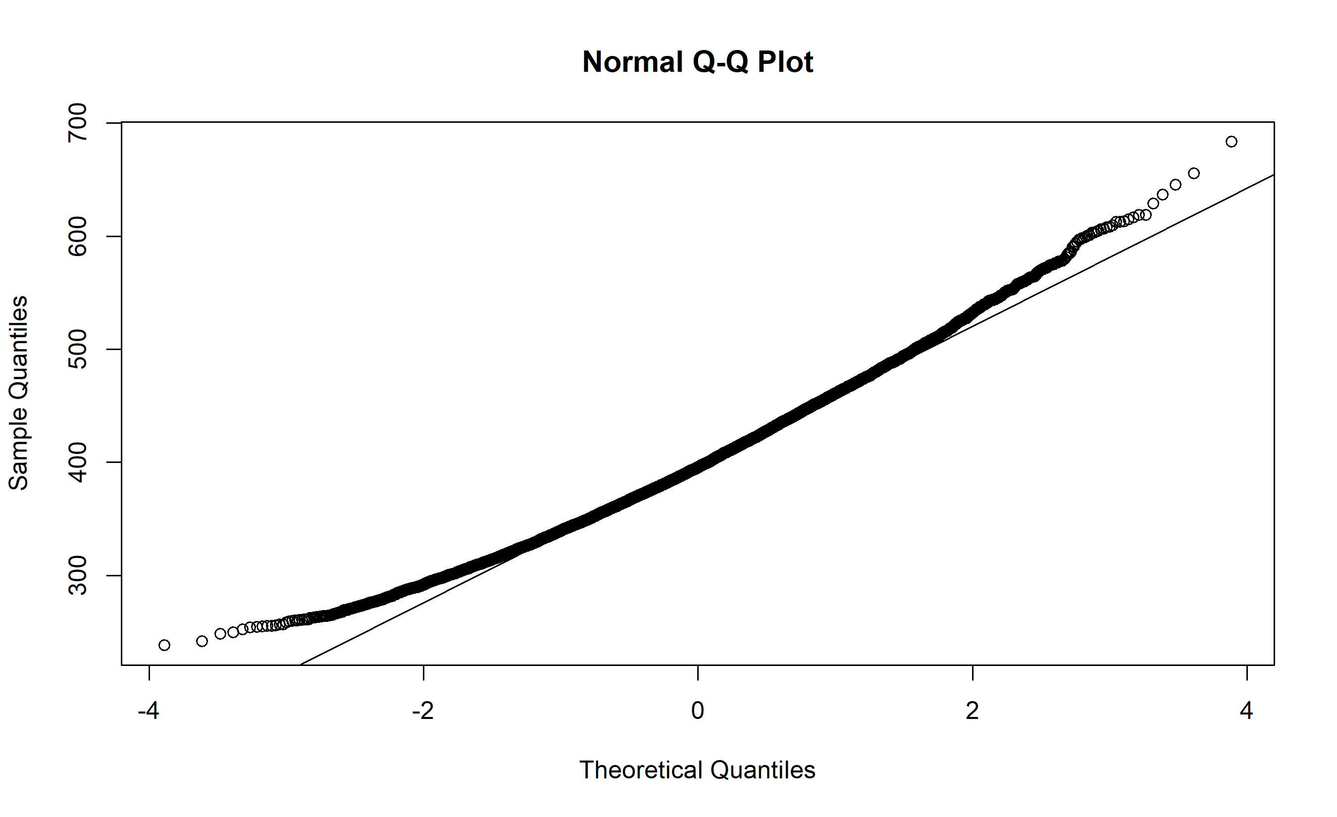
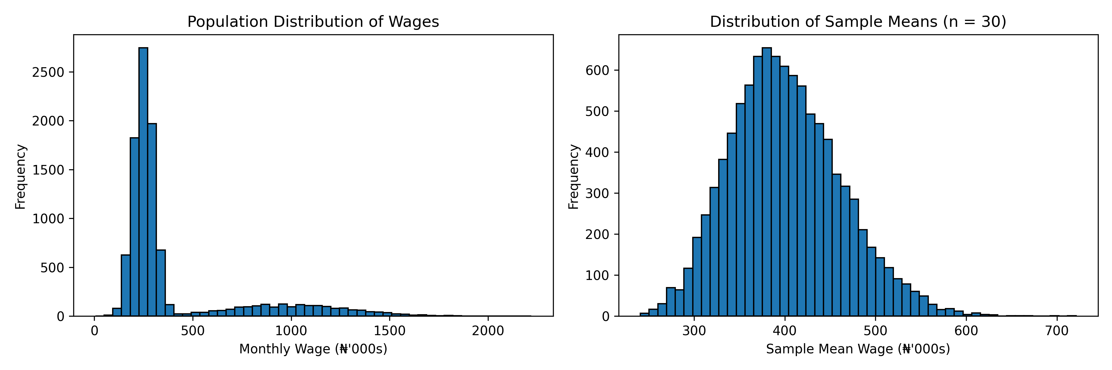
**Key observation:** Although the population distribution is bimodal and non-normal, the distribution of sample means is beautifully normal!
### The Conditions for CLT
1. **Independence:** Samples are drawn independently
2. **Sample size:** Sample size should be "large enough" (typically n ≥ 30, though this depends on how non-normal the population is)
3. **Identical distribution:** All observations come from the same distribution
When these hold, CLT guarantees that sample means are approximately normal, with:
- Mean of sample means: $\mu_{\bar{x}} = \mu$ (the population mean)
- Standard deviation of sample means: $\sigma_{\bar{x}} = \frac{\sigma}{\sqrt{n}}$ (this is called the **standard error**)
### Practical Implication
If the true population mean wage is ₦500k and the population standard deviation is ₦400k, and you survey n = 100 employees:
The sample mean is approximately normal with:
- Mean: 500k
- Standard error: 400k / √100 = 40k
So your sample mean will likely fall within 500k ± 40k = [460k, 540k] (one standard error), and nearly certainly within 500k ± 120k = [380k, 620k] (three standard errors).
---
## Section Review: The Central Limit Theorem
::: {.callout-caution icon="false"}
## 📝 Review Questions: Central Limit Theorem
1. A bank's loan amounts are highly skewed (many small loans, a few large loans). Why does the CLT matter for estimating the average loan amount?
2. You survey 50 random customers about their monthly spending. The sample mean is ₦85,000. Is this the true population mean? How might the CLT help you quantify your uncertainty about the true mean?
3. How does the standard error change as sample size increases? Why is this important for analysts?
4. The CLT says sample means are approximately normal. What conditions must be met for this to be true?
5. A population has mean 100 and standard deviation 25. If you repeatedly sample n=100 observations, what's the approximate standard error of the sample mean?
:::
---
## Confidence Intervals: Quantifying Uncertainty
We rarely know the true population mean. We estimate it from a sample. But the sample mean might be off—that's **sampling error**. How confident should we be in our estimate?
A **confidence interval** is a range of values that, with high confidence (usually 95%), contains the true population parameter.
### The Concept
Imagine you survey 100 Nigerian customers and estimate the average monthly spending at ₦50,000. You're not sure this is exactly right. A 95% confidence interval might be [₦48,000, ₦52,000], meaning: "We're 95% confident the true average lies between ₦48k and ₦52k."
**What does "95% confident" mean?** This is a subtle point often misunderstood.
**Incorrect interpretation:** "There's a 95% probability the true mean is in [₦48k, ₦52k]."
This is wrong because the true mean is fixed (unknown, but fixed). Either it's in the interval or it's not; there's no probability.
**Correct interpretation:** "If we repeated our survey many times, constructing a 95% CI each time, 95% of those intervals would contain the true parameter."
This is a frequentist interpretation: the confidence level refers to the method's long-run behavior, not the probability for a specific interval.
### Constructing a Confidence Interval for the Mean
When you sample from a normal distribution (or when n is large enough by CLT), the sample mean is normally distributed with mean $\mu$ and standard error $\sigma / \sqrt{n}$.
::: {.callout-tip icon="false"}
## 🔑 95% Confidence Interval for the Mean (Known Population σ)
$$\bar{x} \pm z_{0.025} \times \frac{\sigma}{\sqrt{n}}$$
Where $z_{0.025} \approx 1.96$ is the critical value for a 95% confidence level.
In words: sample mean ± 1.96 × standard error
:::
**Example:** You survey 100 Nigerian customers. Sample mean spending: ₦50,000. Population standard deviation (assumed known): ₦10,000.
Standard error: 10,000 / √100 = 1,000
95% CI: 50,000 ± 1.96 × 1,000 = [50,000 ± 1,960] = [₦48,040, ₦51,960]
Interpretation: We're 95% confident the true population mean spending lies between ₦48,040 and ₦51,960.
### The t-Distribution for Small Samples
In practice, we rarely know the population standard deviation $\sigma$. We estimate it from the sample using the sample standard deviation $s$.
When we use $s$ in place of $\sigma$ and have a small sample, the distribution of the sample mean follows a **t-distribution** (named after its developer, William Sealy Gossett, who published under the pseudonym "Student").
The t-distribution is similar to the normal distribution but has heavier tails—it accounts for extra uncertainty from estimating $\sigma$.
::: {.callout-tip icon="false"}
## 🔑 t-Distribution Confidence Interval
$$\bar{x} \pm t_{n-1, \alpha/2} \times \frac{s}{\sqrt{n}}$$
Where $t_{n-1, \alpha/2}$ is the critical value from the t-distribution with $n-1$ degrees of freedom.
:::
For a 95% CI:
- If n = 10: $t_{9, 0.025} \approx 2.262$
- If n = 30: $t_{29, 0.025} \approx 2.045$
- If n = 100: $t_{99, 0.025} \approx 1.984$
- As n → ∞, t approaches the normal value 1.96
**Why degrees of freedom?** When estimating $\sigma$ from sample data, we "lose" one degree of freedom because the sample mean is fixed. A small sample is more uncertain, reflected in a larger critical value.
### Computing Confidence Intervals in R and Python
::: {.panel-tabset}
## R
```{r}
# Sample data: monthly spending for 50 customers
spending <- c(45000, 52000, 48000, 61000, 55000, 42000, 58000,
50000, 47000, 63000, 49000, 51000, 54000, 46000, 60000,
43000, 57000, 52000, 48000, 59000, 41000, 56000,
50000, 44000, 62000, 51000, 49000, 55000, 47000, 64000,
45000, 53000, 50000, 48000, 58000, 42000, 61000,
52000, 46000, 59000, 40000, 57000, 51000, 49000, 63000,
44000, 54000, 50000, 47000, 60000)
# Compute 95% confidence interval using t-distribution
n <- length(spending)
mean_spending <- mean(spending)
se <- sd(spending) / sqrt(n)
df <- n - 1
t_critical <- qt(0.975, df) # 0.975 for two-tailed 95% CI
ci_lower <- mean_spending - t_critical * se
ci_upper <- mean_spending + t_critical * se
cat("Sample mean:", mean_spending, "\n")
cat("Standard error:", se, "\n")
cat("95% Confidence Interval: [", ci_lower, ", ", ci_upper, "]\n")
# Alternatively, use the t.test function
result <- t.test(spending, conf.level = 0.95)
cat("\nUsing t.test function:\n")
print(result)
```
## Python
```{python}
import numpy as np
from scipy import stats
# Sample data: monthly spending
spending = np.array([45000, 52000, 48000, 61000, 55000, 42000, 58000,
50000, 47000, 63000, 49000, 51000, 54000, 46000, 60000,
43000, 57000, 52000, 48000, 59000, 41000, 56000,
50000, 44000, 62000, 51000, 49000, 55000, 47000, 64000,
45000, 53000, 50000, 48000, 58000, 42000, 61000,
52000, 46000, 59000, 40000, 57000, 51000, 49000, 63000,
44000, 54000, 50000, 47000, 60000])
n = len(spending)
mean_spending = np.mean(spending)
se = np.std(spending, ddof=1) / np.sqrt(n)
df = n - 1
t_critical = stats.t.ppf(0.975, df) # 0.975 for two-tailed 95% CI
ci_lower = mean_spending - t_critical * se
ci_upper = mean_spending + t_critical * se
print(f"Sample mean: {mean_spending:.2f}")
print(f"Standard error: {se:.2f}")
print(f"95% Confidence Interval: [{ci_lower:.2f}, {ci_upper:.2f}]")
# Alternatively, use scipy.stats.t.interval
ci = stats.t.interval(0.95, df, loc=mean_spending, scale=se)
print(f"\nUsing scipy.stats.t.interval: [{ci[0]:.2f}, {ci[1]:.2f}]")
```
:::
---
## Section Review: Confidence Intervals
::: {.callout-caution icon="false"}
## 📝 Review Questions: Confidence Intervals
1. A bank surveys 100 customers about monthly savings. Mean: ₦120,000; standard deviation: ₦40,000. Construct a 95% confidence interval for the true population mean savings. Interpret the interval in plain English.
2. Why is the t-distribution used for small samples instead of the normal distribution?
3. How does the width of a confidence interval change as the sample size increases? Why?
4. A politician claims, "The 95% confidence interval shows there's a 95% chance unemployment is between 5% and 8%." Is this correct? Explain the error.
5. You compute a 95% CI and a 99% CI from the same data. Which is wider? Why?
:::
---
## Chapter Summary
This chapter has built a foundation in statistical thinking:
- **Sampling:** Understanding populations, samples, and sampling bias
- **Descriptive statistics:** Using means, medians, and measures of spread to summarize data
- **Probability:** The language of uncertainty, probability rules, and conditional probability
- **Distributions:** Models (Bernoulli, Binomial, Poisson, Normal) that capture randomness
- **Central Limit Theorem:** The guarantee that sample means are normally distributed, even if populations aren't
- **Confidence intervals:** Quantifying uncertainty in our estimates
These concepts underpin everything that follows in this book: hypothesis testing, regression, machine learning. Master these, and the rest flows naturally.
---
## Exercises
::: {.exercises}
#### Chapter 3 Exercises
**1. Populations and Sampling (Recall)**
A Nigerian bank wants to estimate the average loan balance across its 250,000 customers. Explain:
a) Why it's impractical to measure every customer
b) How sampling could provide a good estimate
c) One source of sampling bias the bank should guard against
d) A sampling method that would reduce bias
**2. Central Tendency from Real Data (Comprehension)**
Here's a sample of monthly incomes (in ₦'000s) of 10 Nigerian workers:
150, 180, 160, 200, 900, 165, 155, 170, 175, 160
a) Compute the mean and median
b) Why are they different?
c) Which better represents "typical" income? Justify your answer
**3. Understanding Spread (Comprehension)**
Two investment funds report the same average return (12% annually). Fund A is very consistent (returns 11-13% each year). Fund B is volatile (returns 5% some years, 19% others).
a) Both have the same mean but different standard deviations. Which fund is riskier?
b) An investor might prefer Fund A. Why would understanding spread (not just mean) matter to them?
**4. Probability in Business (Comprehension)**
A call center receives 1,000 customer calls daily. 5% result in a complaint.
a) What's the probability a random caller complains?
b) What's the probability a random caller doesn't complain?
c) If you receive 4 calls, what's the probability all 4 result in complaints? (Assume independence.)
**5. Binomial Distribution (Application)**
An email marketing campaign has a 2% click-through rate. You send 500 emails.
a) How many clicks would you expect, on average?
b) What's the standard deviation of the number of clicks?
c) Is it unusual to get 20 clicks? (Use the normal approximation to the binomial.)
**6. Conditional Probability (Application)**
A bank has 10,000 customers:
- 4,000 have a savings account
- 3,000 have a credit card
- 1,500 have both
a) What's the probability a random customer has a savings account?
b) If you know a customer has a credit card, what's the probability they also have a savings account?
c) Are having a savings account and having a credit card independent? (Hint: check if P(S|C) = P(S).)
**7. The Normal Distribution (Comprehension)**
Customer satisfaction scores at a Nigerian bank are approximately normal with mean 75 and standard deviation 10.
a) Using the 68-95-99.7 rule, estimate the percentage of customers scoring between 55 and 95.
b) Estimate the percentage scoring above 85.
c) If you survey 100 customers, would it be unusual to see a sample mean above 77? Explain.
**8. Central Limit Theorem (Analysis)**
The distribution of daily sales at a retail store is right-skewed (many days with moderate sales, a few very high days). The mean is ₦500k; standard deviation is ₦200k.
a) Is the distribution of daily sales normal? Explain.
b) If you compute the average sales for 50 different days, would the distribution of these 50-day averages be approximately normal? Why?
c) What would be the mean and standard deviation of the distribution of 50-day averages?
**9. Confidence Intervals (Application)**
You survey 64 randomly selected customers at a Lagos store. Average spending: ₦45,000. Sample standard deviation: ₦16,000.
a) Construct a 95% confidence interval for the true population mean spending.
b) Interpret this interval.
c) How would the interval change if you surveyed 256 customers instead of 64 (keeping mean and SD the same)?
**10. Synthesis: The Full Chain (Analysis)**
A bank is considering lowering the interest rate it offers on savings accounts. Before deciding, it wants to estimate the true population mean balance across its customer base.
a) The bank has 500,000 customers. Why not measure all of them?
b) Suggest a sampling method that would reduce bias.
c) Suppose a sample of 100 customers has mean balance ₦2 million with SD ₦800k. Construct a 95% CI.
d) The bank's executives argue the CI is too wide (₦1.84M to ₦2.16M) to make a decision. What sampling change would narrow the interval?
e) Why is this analysis an example of the analytics value chain (data → information → insight → decision)?
:::
---
## Further Reading
- **Whitlock, M. C., & Schluter, D. (2014).** *The Analysis of Biological Data* (2nd ed.). W.H. Freeman. Excellent on foundational statistics with biological examples; many principles transfer to business.
- **Cumming, G. (2012).** *Understanding The New Statistics: Effect Sizes, Confidence Intervals, and Meta-Analysis.* Routledge. Deep dive into confidence intervals and modern approaches to statistical inference.
- **Box, G. E., Hunter, J. S., & Hunter, W. G. (2005).** *Statistics for Experimenters: Design, Innovation, and Discovery* (2nd ed.). Wiley-Interscience. Classic reference on experimental design and statistical thinking.
- **Ross, S. M. (2014).** *Introduction to Probability Models* (11th ed.). Academic Press. Rigorous treatment of probability and distributions.
- **Kahneman, D. (2011).** *Thinking, Fast and Slow.* Farrar, Straus and Giroux. Not purely statistical, but explores human intuition about probability and statistics—essential reading for analysts.
---
## Chapter Appendix: Mathematical Proofs and Derivations
### Appendix 3.A: Why We Divide by n-1 (Not n) in Sample Variance
When computing sample variance, we divide by $n-1$ rather than $n$:
$$s^2 = \frac{1}{n-1} \sum_{i=1}^{n} (x_i - \bar{x})^2$$
Why? Because the sample mean $\bar{x}$ is computed from the same data, it tends to be closer to the data points than the true population mean $\mu$ is. As a result, the sum of squared deviations around $\bar{x}$ is smaller than it would be around $\mu$.
Dividing by $n-1$ instead of $n$ corrects for this bias. With $n-1$, the sample variance $s^2$ is an **unbiased estimator** of the population variance $\sigma^2$.
**Formal proof:** Let $\sigma^2$ be the true population variance. We can show:
$$E\left[\frac{1}{n-1} \sum_{i=1}^{n} (x_i - \bar{x})^2\right] = \sigma^2$$
But:
$$E\left[\frac{1}{n} \sum_{i=1}^{n} (x_i - \bar{x})^2\right] = \frac{n-1}{n} \sigma^2$$
The second formula would systematically underestimate $\sigma^2$. Dividing by $n-1$ corrects this bias. This is why $n-1$ is standard in statistics.
### Appendix 3.B: The Central Limit Theorem—Formal Statement
**Central Limit Theorem:** Let $X_1, X_2, \ldots, X_n$ be independent and identically distributed random variables with mean $\mu$ and variance $\sigma^2$. Let $\bar{X}_n = \frac{1}{n} \sum_{i=1}^{n} X_i$ be the sample mean.
Then, as $n \to \infty$:
$$\frac{\bar{X}_n - \mu}{\sigma / \sqrt{n}} \xrightarrow{d} N(0, 1)$$
In words: the standardized sample mean converges in distribution to a standard normal random variable.
**Intuitive proof (sketch):** The moment generating function of the standardized mean is:
$$M_n(t) = E\left[e^{it(\bar{X}_n - \mu) / (\sigma / \sqrt{n})}\right]$$
By properties of MGFs and Taylor expansion, this converges to the MGF of a standard normal distribution, which is $e^{t^2/2}$. Since the MGF uniquely determines the distribution, the sample mean converges to normal.
### Appendix 3.C: Bayes' Theorem Derivation
Bayes' Theorem follows directly from the definition of conditional probability.
**Start with:** $P(A | B) = \frac{P(A \text{ and } B)}{P(B)}$
**Rearrange:** $P(A \text{ and } B) = P(A | B) \times P(B)$
**Also:** $P(A \text{ and } B) = P(B | A) \times P(A)$
**Therefore:** $P(A | B) \times P(B) = P(B | A) \times P(A)$
**Solve for** $P(A | B)$:
$$P(A | B) = \frac{P(B | A) \times P(A)}{P(B)}$$
This is Bayes' Theorem. Often, we compute $P(B)$ using the law of total probability:
$$P(B) = P(B | A) \times P(A) + P(B | \text{not } A) \times P(\text{not } A)$$
### Appendix 3.D: The t-Distribution and Degrees of Freedom
The t-distribution arises when we standardize the sample mean using the sample standard deviation instead of the population standard deviation:
$$t = \frac{\bar{x} - \mu}{s / \sqrt{n}}$$
This ratio doesn't follow a standard normal distribution (as it would if we used the true $\sigma$). Instead, it follows a t-distribution with $n-1$ degrees of freedom.
**Why $n-1$ degrees of freedom?**
When we estimate $\sigma$ with $s$ from the same sample, we've "used up" one degree of freedom (the constraint that deviations sum to zero: $\sum (x_i - \bar{x}) = 0$). We have $n$ observations but only $n-1$ independent deviations.
As $n \to \infty$, the sample standard deviation $s$ becomes an excellent estimate of $\sigma$, and the t-distribution converges to the normal distribution. For n = 100, the difference is negligible; for n = 10, it matters.
### Appendix 3.E: Proof of the 95% Confidence Interval
Suppose $X_1, \ldots, X_n$ are i.i.d. $N(\mu, \sigma^2)$ with known $\sigma$.
The sample mean $\bar{X}$ is normally distributed: $\bar{X} \sim N(\mu, \sigma^2/n)$.
Standardizing: $Z = \frac{\bar{X} - \mu}{\sigma / \sqrt{n}} \sim N(0, 1)$
For a 95% CI, we want $P(|Z| \leq z_{0.025}) = 0.95$. From the standard normal table, $z_{0.025} = 1.96$.
$$P\left(|Z| \leq 1.96\right) = 0.95$$
$$P\left(\left|\frac{\bar{X} - \mu}{\sigma / \sqrt{n}}\right| \leq 1.96\right) = 0.95$$
$$P\left(\bar{X} - 1.96 \frac{\sigma}{\sqrt{n}} \leq \mu \leq \bar{X} + 1.96 \frac{\sigma}{\sqrt{n}}\right) = 0.95$$
The 95% CI is: $\bar{X} \pm 1.96 \frac{\sigma}{\sqrt{n}}$
This interval traps the true $\mu$ with probability 0.95 (over repeated sampling). In the long run, 95% of such intervals contain the true parameter.