---
title: "Bayesian Thinking in Business Analytics"
---

```{python}
#| label: python-setup-56-bayesian-methods
#| include: false

import numpy as np
import pandas as pd
import matplotlib.pyplot as plt
import seaborn as sns
from scipy.stats import beta
```


::: {.callout-note icon="false"}
## 📋 Learning Objectives

By the end of this chapter, you will:
- Understand probability as degree of belief (Bayesian) vs. long-run frequency (Frequentist)
- Apply Bayes' theorem to sequential decision-making with data updates
- Use conjugate priors for efficient computation (Beta-Binomial, Normal-Normal, Gamma-Poisson)
- Build Bayesian regression models with credible intervals (not confidence intervals)
- Apply probabilistic programming (Stan, PyMC) for complex models
- Update beliefs sequentially as new data arrives
- Make credible inferences about parameters, not just reject/fail-to-reject null hypotheses

:::

## What Is Bayesian Statistics? Learning from Experience

Suppose you are a loan officer at a microfinance institution in Kano. A new applicant, Mr Musa, sits across from you. You have no transaction history for him — he is a first-time borrower. But you are not completely in the dark. You know that, historically, traders in his market segment have a 15% default rate. You also notice that he has a well-organised account book, offers collateral, and his references check out. How should you use this background knowledge together with the new information in front of you?

This is Bayesian reasoning in everyday life. You start with a **prior belief** based on existing knowledge ("traders in this category default 15% of the time"). You observe **new evidence** (his behaviour, records, and references). You update your belief to produce a **posterior** — a revised estimate of his default risk that combines both the background knowledge and the new evidence. If his individual signals are strong, your posterior belief shifts toward "this person is a better-than-average risk." If his signals are weak or mixed, your posterior stays close to the 15% prior.

Bayesian statistics formalises this intuitive process into mathematics. It is not a radically different kind of statistics from what you have learned so far — it is the same probability theory applied in a different way. The key difference is philosophical: **Bayesian statistics treats uncertainty about unknown quantities as probability distributions that can be updated as new data arrives**. This means you can answer questions like "Given everything I know, what is the probability that this borrower defaults?" rather than "If I repeat this experiment infinitely many times, how often would my test reject the null hypothesis?"

This distinction matters enormously for business. In the real world, you do not run an infinite number of experiments. You make one decision per customer, per product launch, per marketing campaign. You want to incorporate everything you already know (prior knowledge) and combine it with the specific data in front of you (likelihood) to arrive at the best possible belief about the unknown quantity (posterior). This is exactly what Bayesian statistics does.

### Two Ways to Think About Probability

There are two ways to interpret probability, and understanding their difference is the key to understanding Bayesian statistics.

**Frequentist probability** (what you learned in Chapter 6) says: probability is the long-run frequency of an event if you repeated an experiment many times. The probability of a coin landing heads is 0.5 because, if you flipped it a million times, half would be heads. This interpretation works well for repeatable experiments. But it becomes awkward when the event is a one-time decision: "What is the probability that this specific merger succeeds?" — you cannot repeat the merger a million times to find out.

**Bayesian probability** is broader: probability is a measure of **degree of belief** about an uncertain quantity. You can have a probability distribution over "will this merger succeed?" based on your knowledge and analysis, even though the event happens only once. As you gather more evidence (due diligence reports, market analysis, regulatory signals), you update that probability. This is perfectly natural and reflects how thoughtful decision-makers actually reason.

In practice, for large datasets and standard problems, Bayesian and frequentist methods often give very similar answers. The Bayesian approach becomes distinctly more valuable when: (i) data is scarce and prior knowledge is important; (ii) you need to update beliefs sequentially as data arrives; (iii) you want a direct probability statement about the parameter of interest rather than a p-value. As a Nigerian bank makes credit decisions on new customers continuously, a Bayesian approach updates the default probability model daily, automatically incorporating new patterns — something frequentist batch methods cannot do efficiently.

Philosophically, Bayesian thinking reflects how humans actually learn: start with a prior belief (a borrower's market segment has historically had a 10% default rate), observe new data (this particular borrower's payment behaviour and collateral), update your belief (perhaps their default risk is now assessed at 7%), and make a decision based on the posterior.

## Bayes' Theorem from First Principles

Bayes' theorem is derived from the definition of conditional probability. If $A$ and $B$ are events:

$$
P(A | B) = \frac{P(B | A) P(A)}{P(B)}
$$

where:
- $P(A | B)$ = posterior: probability of $A$ given we observed $B$
- $P(B | A)$ = likelihood: probability of observing $B$ if $A$ is true
- $P(A)$ = prior: our belief in $A$ before seeing data
- $P(B)$ = marginal likelihood: probability of observing $B$ under all possible values of $A$

**The medical test example**: A disease has prevalence 1% (1 in 100 people). A test is 95% sensitive (detects 95% of diseased) and 90% specific (correctly identifies 90% of healthy). You test positive. What is the probability you have the disease?

Using Bayes:
$$
P(\text{Disease} | \text{Positive}) = \frac{P(\text{Positive} | \text{Disease}) \times P(\text{Disease})}{P(\text{Positive})}
$$

$$
= \frac{0.95 \times 0.01}{0.95 \times 0.01 + 0.10 \times 0.99} = \frac{0.0095}{0.0095 + 0.099} \approx 0.087
$$

So despite the positive test, there's only an 8.7% chance you have the disease! This is the "base rate fallacy"—the low prior probability dominates. This intuition is crucial for business: a model predicting a rare event (fraud, equipment failure) must have very high precision to be useful.

::: {.callout-note icon="false"}
## 📘 Theory: Bayes' Theorem for Continuous Parameters

For a continuous parameter $\theta$ and observed data $y$:

$$
p(\theta | y) = \frac{p(y | \theta) p(\theta)}{p(y)}
$$

where $p(\theta)$ is the prior, $p(y|\theta)$ is the likelihood, and $p(\theta|y)$ is the posterior. The denominator is the marginal likelihood:

$$
p(y) = \int p(y | \theta) p(\theta) d\theta
$$

Often intractable, but proportionality suffices: $p(\theta | y) \propto p(y | \theta) p(\theta)$.

:::

::: {.callout-tip icon="false"}
## 🔑 Key Formula

$$\text{Posterior} \propto \text{Likelihood} \times \text{Prior}$$

:::

::: {.panel-tabset}

## R

```{r}
#| label: ch56-bayes-theorem
library(tidyverse)

# Example: Bayesian updating of default probability for Nigerian microfinance borrowers
# Prior: historical default rate in the zone is 15%
prior_prob_default <- 0.15

# Test: credit bureau data shows positive history
# Likelihood: P(positive history | default) = 0.3 (30% of defaulters have spotty history)
#           P(positive history | no default) = 0.9 (90% of non-defaulters have clean history)
likelihood_given_default <- 0.3
likelihood_given_no_default <- 0.9

# Marginal likelihood
marginal_likelihood <- (likelihood_given_default * prior_prob_default) +
                       (likelihood_given_no_default * (1 - prior_prob_default))

# Posterior
posterior_prob_default <- (likelihood_given_default * prior_prob_default) / marginal_likelihood

cat("\n=== Bayesian Update: Borrower Default Risk ===\n")
cat("Prior P(default):", round(prior_prob_default, 3), "\n")
cat("Likelihood P(clean history | no default):", round(likelihood_given_no_default, 3), "\n")
cat("Posterior P(default | clean history):", round(posterior_prob_default, 3), "\n")
cat("Risk reduction:", round((prior_prob_default - posterior_prob_default) / prior_prob_default * 100, 1), "%\n")

# Sequential update: borrower has made 12 consecutive on-time payments
# Each payment updates the belief
n_payments <- 12
prob_payment_given_default <- 0.3  # Defaulters sometimes make sporadic payments
prob_payment_given_no_default <- 0.98  # Non-defaulters almost always pay on time

current_posterior <- posterior_prob_default

cat("\n=== Sequential Updates ===\n")
for (payment in 1:n_payments) {
  # Bayes update for this payment
  likelihood <- (prob_payment_given_default * current_posterior) +
                (prob_payment_given_no_default * (1 - current_posterior))
  current_posterior <- (prob_payment_given_default * current_posterior) / likelihood

  if (payment %in% c(1, 3, 6, 12)) {
    cat("After payment", payment, "- P(default) =", round(current_posterior, 4), "\n")
  }
}

cat("\nFinal posterior after 12 payments: P(default) =", round(current_posterior, 4), "\n")
```

## Python

```{python}
#| label: py-ch56-bayes-theorem
import numpy as np

# Bayesian update: default probability
prior = 0.15
likelihood_default = 0.3
likelihood_no_default = 0.9

marginal = likelihood_default * prior + likelihood_no_default * (1 - prior)
posterior = (likelihood_default * prior) / marginal

print("\n=== Bayesian Update: Borrower Default Risk ===")
print(f"Prior P(default): {prior:.3f}")
print(f"Likelihood P(clean history | no default): {likelihood_no_default:.3f}")
print(f"Posterior P(default | clean history): {posterior:.3f}")
print(f"Risk reduction: {(prior - posterior) / prior * 100:.1f}%")

# Sequential updates
current_posterior = posterior
prob_pay_default = 0.3
prob_pay_no_default = 0.98

print("\n=== Sequential Updates (12 Payments) ===")
for i in range(1, 13):
    likelihood = prob_pay_default * current_posterior + prob_pay_no_default * (1 - current_posterior)
    current_posterior = (prob_pay_default * current_posterior) / likelihood

    if i in [1, 3, 6, 12]:
        print(f"After payment {i}: P(default) = {current_posterior:.4f}")

print(f"\nFinal posterior: P(default) = {current_posterior:.4f}")
```

:::

## The Prior, Likelihood, and Posterior

**Prior**: Your belief before seeing data. For a new loan applicant in Lagos, the prior might be the historical default rate in Lagos (say, 12%). This can be informative (based on years of data) or vague (weak information).

**Likelihood**: How probable is the observed data under different parameter values? For a borrower with 12 months of on-time payments, the likelihood of observing this given they will eventually default is low (0.3^12); given they will not default, it is high (0.98^12).

**Posterior**: Your updated belief after seeing data. The ratio of posterior to prior is driven by the likelihood ratio. As more data arrives, the posterior becomes more concentrated.

Key insight: with enough data, the posterior is dominated by the likelihood, and the prior "forgets." With sparse data, the prior remains influential.

## Conjugate Priors

Some prior-likelihood combinations have a posterior in the same family, enabling analytical updates without numerical integration.

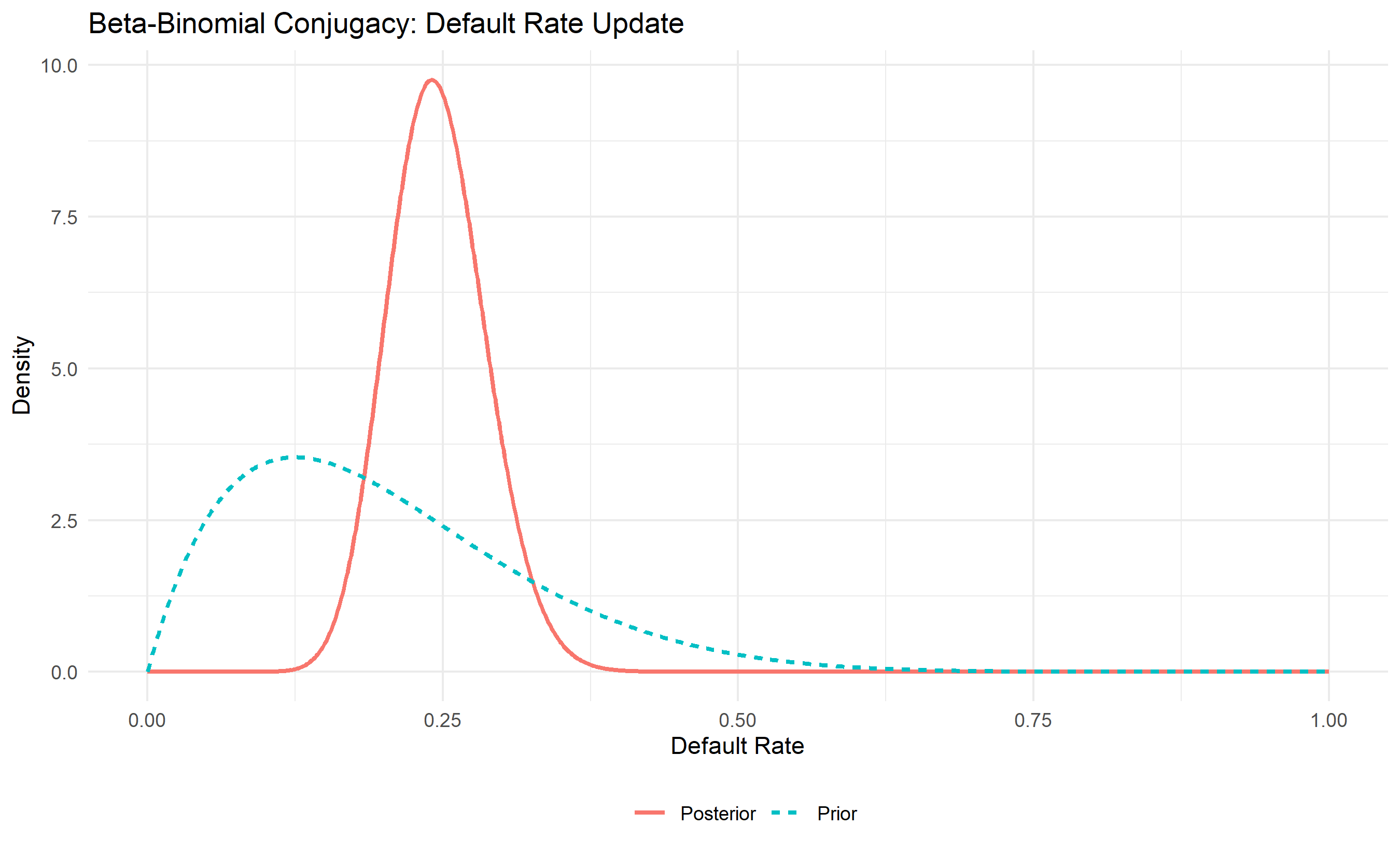
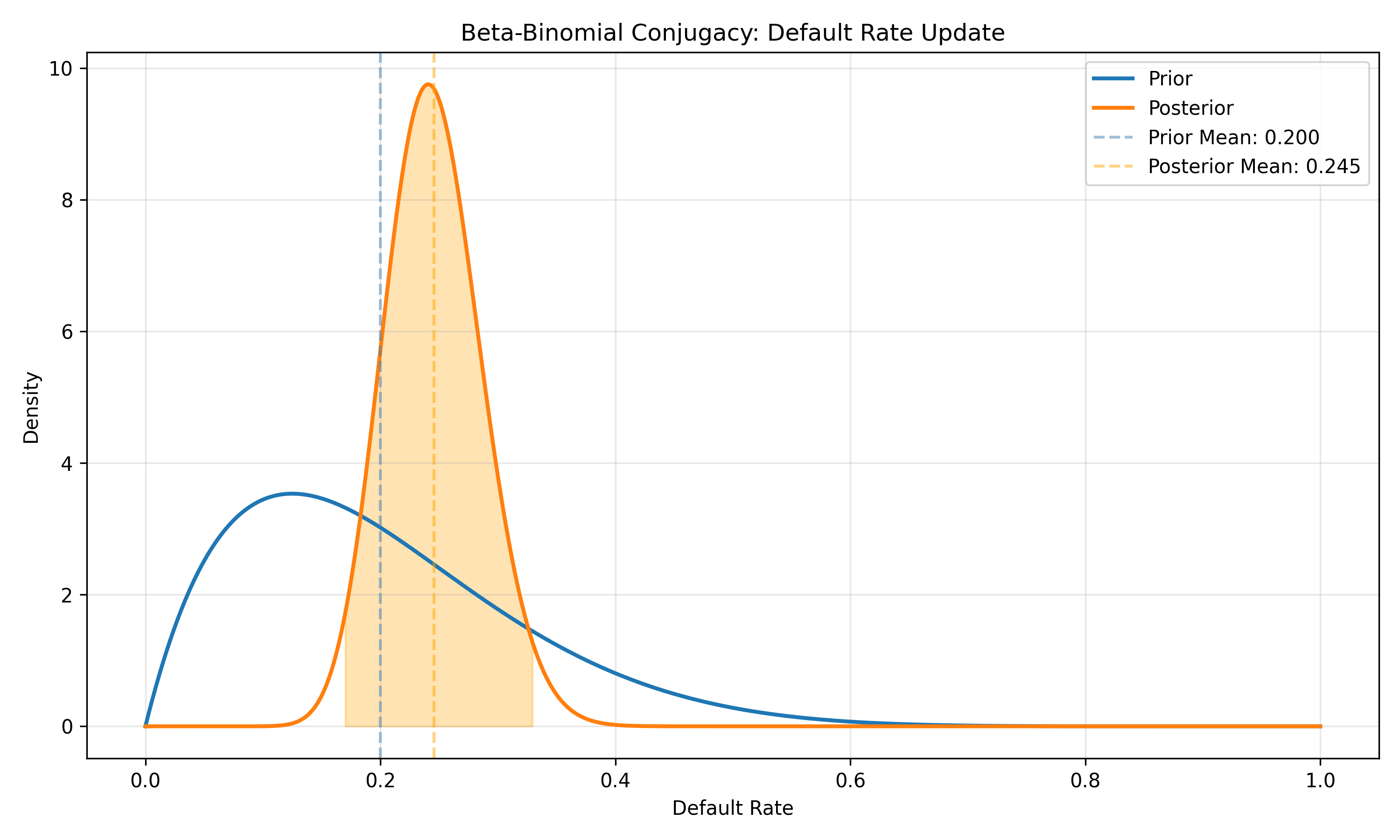
**Beta-Binomial**: Prior $\theta \sim \text{Beta}(\alpha, \beta)$, likelihood is Binomial. Posterior is $\text{Beta}(\alpha + \text{successes}, \beta + \text{failures})$. Example: estimate the probability a customer defaults (binary outcome). Prior: $\text{Beta}(2, 8)$ (expecting ~20% default). Observe 15 defaults, 85 no-defaults in new cohort. Posterior: $\text{Beta}(2 + 15, 8 + 85) = \text{Beta}(17, 93)$, with posterior mean = $17 / 110 = 0.155$.

**Normal-Normal**: Prior and likelihood are both Normal. Posterior is Normal with mean = weighted average of prior mean and data mean.

**Gamma-Poisson**: Prior $\lambda \sim \text{Gamma}(\alpha, \beta)$, likelihood is Poisson. Posterior is $\text{Gamma}(\alpha + \text{sum of counts}, \beta + n)$.

::: {.panel-tabset}

## R

```{r}
#| label: ch56-conjugate-priors
library(tidyverse)

# Beta-Binomial conjugacy
# Prior: Beta(2, 8) - expect ~20% default rate
prior_alpha <- 2
prior_beta <- 8

# Observed data: 25 defaults, 75 non-defaults
observed_defaults <- 25
observed_non_defaults <- 75

# Posterior
post_alpha <- prior_alpha + observed_defaults
post_beta <- prior_beta + observed_non_defaults

# Prior and posterior means
prior_mean <- prior_alpha / (prior_alpha + prior_beta)
post_mean <- post_alpha / (post_alpha + post_beta)

cat("\n=== Beta-Binomial Conjugacy ===\n")
cat("Prior Beta(α=", prior_alpha, ", β=", prior_beta, ")\n")
cat("Prior mean (expected default rate):", round(prior_mean, 3), "\n")
cat("Observed: ", observed_defaults, " defaults out of ", observed_defaults + observed_non_defaults, "\n")
cat("Observed default rate:", round(observed_defaults / (observed_defaults + observed_non_defaults), 3), "\n")
cat("Posterior Beta(α=", post_alpha, ", β=", post_beta, ")\n")
cat("Posterior mean:", round(post_mean, 3), "\n")

# Credible interval (Bayesian confidence interval)
lower <- qbeta(0.025, post_alpha, post_beta)
upper <- qbeta(0.975, post_alpha, post_beta)

cat("\n95% Credible Interval:", round(lower, 3), "to", round(upper, 3), "\n")
cat("Interpretation: Given the data, the default rate is between",
    round(lower * 100, 1), "% and", round(upper * 100, 1), "% with 95% probability.\n")

# Visualization
x <- seq(0, 1, length.out = 1000)
prior_density <- dbeta(x, prior_alpha, prior_beta)
post_density <- dbeta(x, post_alpha, post_beta)

n_pts <- length(x)
ggplot(tibble(x = rep(x, 2), density = c(prior_density, post_density),
              distribution = rep(c("Prior", "Posterior"), each = n_pts)),
       aes(x = x, y = density, color = distribution, linetype = distribution)) +
  geom_line(linewidth = 1) +
  labs(
    title = "Beta-Binomial Conjugacy: Default Rate Update",
    x = "Default Rate", y = "Density",
    color = "", linetype = ""
  ) +
  theme_minimal() +
  theme(legend.position = "bottom")
```

## Python

```{python}
#| label: py-ch56-conjugate-priors
import numpy as np
from scipy.stats import beta
import matplotlib.pyplot as plt

# Beta-Binomial
prior_alpha, prior_beta = 2, 8
observed_defaults, observed_non_defaults = 25, 75

post_alpha = prior_alpha + observed_defaults
post_beta = prior_beta + observed_non_defaults

prior_mean = prior_alpha / (prior_alpha + prior_beta)
post_mean = post_alpha / (post_alpha + post_beta)
observed_rate = observed_defaults / (observed_defaults + observed_non_defaults)

print("\n=== Beta-Binomial Conjugacy ===")
print(f"Prior Beta(α={prior_alpha}, β={prior_beta})")
print(f"Prior mean: {prior_mean:.3f}")
print(f"Observed default rate: {observed_rate:.3f}")
print(f"Posterior Beta(α={post_alpha}, β={post_beta})")
print(f"Posterior mean: {post_mean:.3f}")

# Credible interval
lower = beta.ppf(0.025, post_alpha, post_beta)
upper = beta.ppf(0.975, post_alpha, post_beta)

print(f"\n95% Credible Interval: {lower:.3f} to {upper:.3f}")
print(f"Interpretation: Default rate is between {lower*100:.1f}% and {upper*100:.1f}% with 95% probability")

# Visualization
x = np.linspace(0, 1, 1000)
prior_density = beta.pdf(x, prior_alpha, prior_beta)
post_density = beta.pdf(x, post_alpha, post_beta)

fig, ax = plt.subplots(figsize=(10, 6))
ax.plot(x, prior_density, label='Prior', linewidth=2)
ax.plot(x, post_density, label='Posterior', linewidth=2)
ax.axvline(prior_mean, color='steelblue', linestyle='--', alpha=0.5, label=f'Prior Mean: {prior_mean:.3f}')
ax.axvline(post_mean, color='orange', linestyle='--', alpha=0.5, label=f'Posterior Mean: {post_mean:.3f}')
ax.fill_between(x[(x >= lower) & (x <= upper)], 0,
                post_density[(x >= lower) & (x <= upper)], alpha=0.3, color='orange')
ax.set_xlabel('Default Rate')
ax.set_ylabel('Density')
ax.set_title('Beta-Binomial Conjugacy: Default Rate Update')
ax.legend()
ax.grid(True, alpha=0.3)
plt.tight_layout()
plt.show()
```

:::

## Bayesian Regression

Ordinary regression gives point estimates of coefficients. Bayesian regression gives posterior distributions. For a simple linear regression $y = \alpha + \beta x + \epsilon$ with $\epsilon \sim N(0, \sigma^2)$, assign priors to $\alpha$, $\beta$, and $\sigma$. The posterior is a distribution, and credible intervals (not confidence intervals) are interpretable.

Unlike frequentist CIs, a Bayesian credible interval directly states: "The coefficient is in this range with 95% probability given the data and prior."

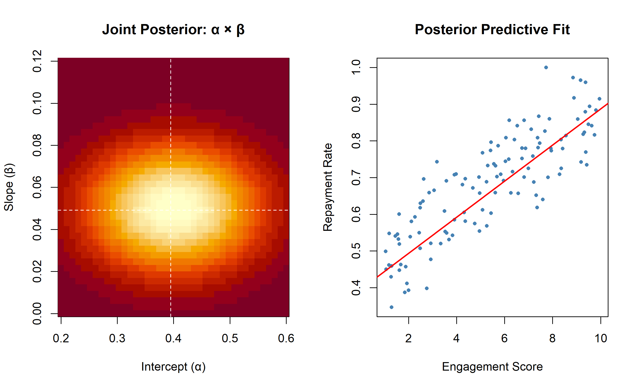
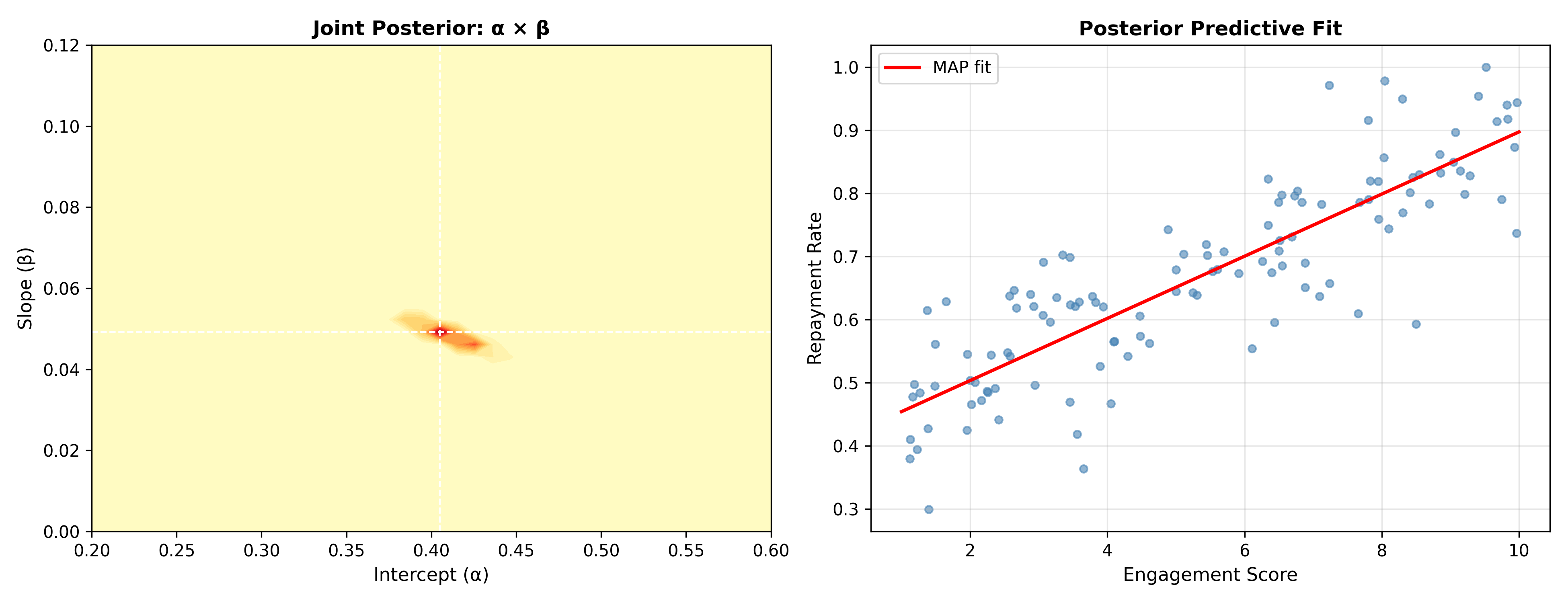
We demonstrate Bayesian simple linear regression using grid approximation (no external MCMC package required). The setting: predict monthly loan repayment rate from customer engagement score for a Nigerian microfinance bank.

::: {.panel-tabset}

## R

```{r}
#| label: ch56-bayesian-regression
library(tidyverse)

set.seed(8273)

# Simulate data: loan repayment rate ~ engagement score
n_obs       <- 120
engagement  <- runif(n_obs, 1, 10)
repay_rate  <- 0.40 + 0.05 * engagement + rnorm(n_obs, 0, 0.08)
repay_rate  <- pmin(pmax(repay_rate, 0.05), 1.00)

loan_df <- tibble(engagement = engagement, repay_rate = repay_rate)

# --- Grid approximation for Bayesian linear regression ---
# Model: repay_rate = alpha + beta * engagement + eps, eps ~ N(0, sigma^2)
# Priors: alpha ~ N(0.40, 0.10), beta ~ N(0.05, 0.02), sigma ~ Uniform(0.01, 0.30)

alpha_grid <- seq(0.20, 0.60, length.out = 40)
beta_grid  <- seq(0.00, 0.12, length.out = 40)
sigma      <- 0.08  # fix sigma at MLE estimate for 2D grid

# Compute log-posterior on grid
log_post <- outer(alpha_grid, beta_grid, FUN = function(a, b) {
  log_prior    <- dnorm(a, 0.40, 0.10, log = TRUE) + dnorm(b, 0.05, 0.02, log = TRUE)
  fitted       <- a + b * engagement
  log_lik      <- sum(dnorm(repay_rate, mean = fitted, sd = sigma, log = TRUE))
  log_prior + log_lik
})

# Normalise to get posterior probabilities
post_prob <- exp(log_post - max(log_post))
post_prob <- post_prob / sum(post_prob)

# Marginal posteriors
alpha_marginal <- rowSums(post_prob)
beta_marginal  <- colSums(post_prob)

alpha_map <- alpha_grid[which.max(alpha_marginal)]
beta_map  <- beta_grid[which.max(beta_marginal)]

# 95% credible intervals
alpha_cdf <- cumsum(alpha_marginal) / sum(alpha_marginal)
alpha_ci  <- c(alpha_grid[which(alpha_cdf >= 0.025)[1]],
               alpha_grid[which(alpha_cdf >= 0.975)[1]])

beta_cdf  <- cumsum(beta_marginal) / sum(beta_marginal)
beta_ci   <- c(beta_grid[which(beta_cdf >= 0.025)[1]],
               beta_grid[which(beta_cdf >= 0.975)[1]])

cat("=== Bayesian Linear Regression (Grid Approximation) ===\n")
cat("Intercept (alpha):\n")
cat("  MAP estimate:", round(alpha_map, 4), "\n")
cat("  95% Credible Interval:", round(alpha_ci, 4), "\n")
cat("\nSlope (beta, per unit engagement):\n")
cat("  MAP estimate:", round(beta_map, 4), "\n")
cat("  95% Credible Interval:", round(beta_ci, 4), "\n")
cat("\nInterpretation: a 1-unit increase in engagement raises expected\n")
cat("repayment rate by", round(beta_map * 100, 1), "pp (95% CI:",
    round(beta_ci[1] * 100, 1), "–", round(beta_ci[2] * 100, 1), "pp)\n")

# Visualise: posterior over (alpha, beta) + data
par(mfrow = c(1, 2))
image(alpha_grid, beta_grid, post_prob,
      main = "Joint Posterior: α × β",
      xlab = "Intercept (α)", ylab = "Slope (β)",
      col  = hcl.colors(20, "YlOrRd"))
abline(v = alpha_map, h = beta_map, lty = 2, col = "white")

plot(engagement, repay_rate,
     col = "steelblue", pch = 16, cex = 0.7,
     main = "Posterior Predictive Fit",
     xlab = "Engagement Score", ylab = "Repayment Rate")
abline(a = alpha_map, b = beta_map, col = "red", lwd = 2)
par(mfrow = c(1, 1))
```

## Python

```{python}
#| label: py-ch56-bayesian-regression
import numpy as np
import matplotlib.pyplot as plt

np.random.seed(8273)

# Simulate data
n_obs      = 120
engagement = np.random.uniform(1, 10, n_obs)
repay_rate = np.clip(0.40 + 0.05 * engagement + np.random.normal(0, 0.08, n_obs), 0.05, 1.0)

# Grid approximation
alpha_grid = np.linspace(0.20, 0.60, 40)
beta_grid  = np.linspace(0.00, 0.12, 40)
sigma      = 0.08

# Log-posterior
AA, BB = np.meshgrid(alpha_grid, beta_grid, indexing='ij')
log_prior = (-(AA - 0.40)**2 / (2 * 0.10**2) +
             -(BB - 0.05)**2 / (2 * 0.02**2))

# Vectorised log-likelihood
fitted    = AA[:, :, np.newaxis] + BB[:, :, np.newaxis] * engagement[np.newaxis, np.newaxis, :]
log_lik   = np.sum(-0.5 * ((repay_rate - fitted) / sigma)**2, axis=2)

log_post  = log_prior + log_lik
post      = np.exp(log_post - log_post.max())
post     /= post.sum()

# Marginals
alpha_marg = post.sum(axis=1)
beta_marg  = post.sum(axis=0)

alpha_map  = alpha_grid[alpha_marg.argmax()]
beta_map   = beta_grid[beta_marg.argmax()]

# Credible intervals
alpha_cdf  = np.cumsum(alpha_marg) / alpha_marg.sum()
beta_cdf   = np.cumsum(beta_marg) / beta_marg.sum()
alpha_ci   = (alpha_grid[np.searchsorted(alpha_cdf, 0.025)],
              alpha_grid[np.searchsorted(alpha_cdf, 0.975)])
beta_ci    = (beta_grid[np.searchsorted(beta_cdf, 0.025)],
              beta_grid[np.searchsorted(beta_cdf, 0.975)])

print("=== Bayesian Linear Regression (Grid Approximation) ===")
print(f"Intercept MAP: {alpha_map:.4f},  95% CI: [{alpha_ci[0]:.4f}, {alpha_ci[1]:.4f}]")
print(f"Slope MAP:     {beta_map:.4f},   95% CI: [{beta_ci[0]:.4f}, {beta_ci[1]:.4f}]")
print(f"\nInterpretation: 1-unit engagement → +{beta_map*100:.1f}pp repayment rate")
print(f"  (95% CI: {beta_ci[0]*100:.1f} – {beta_ci[1]*100:.1f} pp)")

# Visualise
fig, (ax1, ax2) = plt.subplots(1, 2, figsize=(13, 5))

ax1.contourf(alpha_grid, beta_grid, post.T, levels=20, cmap='YlOrRd')
ax1.axvline(alpha_map, color='white', linestyle='--', linewidth=1)
ax1.axhline(beta_map,  color='white', linestyle='--', linewidth=1)
ax1.set_xlabel('Intercept (α)', fontsize=11)
ax1.set_ylabel('Slope (β)',     fontsize=11)
ax1.set_title('Joint Posterior: α × β', fontweight='bold')

x_line = np.linspace(1, 10, 100)
ax2.scatter(engagement, repay_rate, s=20, alpha=0.6, color='steelblue')
ax2.plot(x_line, alpha_map + beta_map * x_line, color='red',
         linewidth=2, label='MAP fit')
ax2.set_xlabel('Engagement Score', fontsize=11)
ax2.set_ylabel('Repayment Rate', fontsize=11)
ax2.set_title('Posterior Predictive Fit', fontweight='bold')
ax2.legend()
ax2.grid(alpha=0.3)

plt.tight_layout()
plt.show()
```

:::

## Probabilistic Programming: Stan and PyMC

For complex models, analytical posteriors don't exist. Markov Chain Monte Carlo (MCMC) algorithms sample from the posterior numerically. Stan (R) and PyMC (Python) are languages where you write the model generatively, and the software automatically generates MCMC samplers.

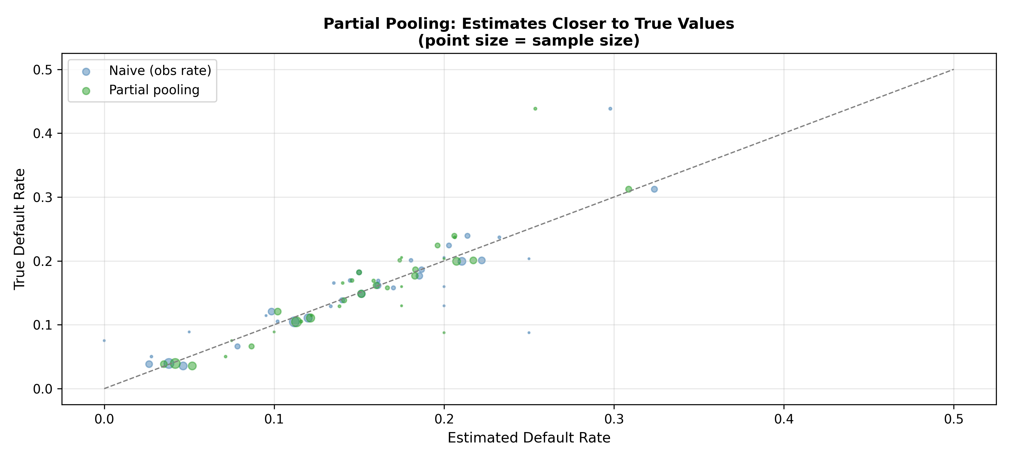
The example below shows a **conceptual** Stan/PyMC model for a hierarchical default-rate analysis (50 Nigerian states, each with its own default rate, drawn from a common national distribution). We show the model specification and explain the output rather than running the full MCMC, which can take several minutes.

::: {.panel-tabset}

## R

```{r}
#| label: ch56-probabilistic-programming-concept
cat("=== Hierarchical Bayesian Model: Default Rates Across States ===\n\n")

cat("Stan model specification (conceptual — not executed):\n")
cat("────────────────────────────────────────────────────\n")
cat("data {\n")
cat("  int<lower=0> N_states;             // number of states (50)\n")
cat("  int<lower=0> n[N_states];          // loans per state\n")
cat("  int<lower=0> k[N_states];          // defaults per state\n")
cat("}\n\n")
cat("parameters {\n")
cat("  real<lower=0,upper=1> mu;          // national mean default rate\n")
cat("  real<lower=0>         kappa;       // concentration (higher = less pooling)\n")
cat("  real<lower=0,upper=1> theta[N_states]; // state-level default rates\n")
cat("}\n\n")
cat("model {\n")
cat("  mu    ~ beta(2, 8);                // prior: ~20% national default rate\n")
cat("  kappa ~ exponential(0.1);\n")
cat("  for (s in 1:N_states) {\n")
cat("    theta[s] ~ beta(mu * kappa, (1 - mu) * kappa);  // hyperprior\n")
cat("    k[s]     ~ binomial(n[s], theta[s]);             // likelihood\n")
cat("  }\n")
cat("}\n\n")

cat("Key idea: partial pooling\n")
cat("  - States with many loans: posterior theta[s] ≈ observed default rate\n")
cat("  - States with few loans: posterior theta[s] shrinks toward national mu\n")
cat("  - This prevents noisy estimates for data-sparse states\n\n")

# Simulate what the hierarchical model would produce
set.seed(9147)
n_states  <- 36  # Nigeria's 36 states
mu_true   <- 0.15
kappa     <- 20   # concentration

# Each state has a true default rate drawn from the hyperprior
theta_true <- rbeta(n_states, mu_true * kappa, (1 - mu_true) * kappa)

# Observed data (variable sample sizes across states)
n_loans   <- round(rexp(n_states, 1 / 200)) + 20
k_defaults<- rbinom(n_states, n_loans, theta_true)
obs_rate  <- k_defaults / n_loans

# Naive estimate vs partial pooling (James-Stein shrinkage approximation)
pooled_estimate <- (k_defaults + mu_true * kappa) / (n_loans + kappa)

state_df <- tibble(
  state        = paste0("State_", 1:n_states),
  n_loans      = n_loans,
  k_defaults   = k_defaults,
  obs_rate     = obs_rate,
  pooled_est   = pooled_estimate,
  true_rate    = theta_true
)

cat("=== Partial Pooling Effect (Simulated) ===\n")
cat(sprintf("%-12s %8s %10s %10s %10s\n",
            "State", "n_loans", "Obs Rate", "Pooled", "True Rate"))
cat(paste(rep("-", 54), collapse = ""), "\n")
for (i in 1:10) {
  cat(sprintf("%-12s %8d %10.3f %10.3f %10.3f\n",
              state_df$state[i], state_df$n_loans[i],
              state_df$obs_rate[i], state_df$pooled_est[i],
              state_df$true_rate[i]))
}

# RMSE comparison
rmse_naive  <- sqrt(mean((obs_rate - theta_true)^2))
rmse_pooled <- sqrt(mean((pooled_estimate - theta_true)^2))
cat(sprintf("\nRMSE (naive observed rate): %.4f\n", rmse_naive))
cat(sprintf("RMSE (partial pooling):     %.4f\n", rmse_pooled))
cat(sprintf("Improvement:                %.1f%%\n", (rmse_naive - rmse_pooled) / rmse_naive * 100))
```

## Python

```{python}
#| label: py-ch56-probabilistic-programming-concept
import numpy as np
import pandas as pd
import matplotlib.pyplot as plt

print("=== Hierarchical Bayesian Model: State-Level Default Rates ===\n")

print("PyMC model specification (conceptual — not executed):")
print("─" * 54)
print("import pymc as pm")
print("")
print("with pm.Model() as hierarchical_model:")
print("    # Hyperpriors (national distribution)")
print("    mu    = pm.Beta('mu', alpha=2, beta=8)")
print("    kappa = pm.Exponential('kappa', lam=0.1)")
print("")
print("    # State-level default rates")
print("    theta = pm.Beta('theta', alpha=mu*kappa,")
print("                            beta=(1-mu)*kappa, shape=N_states)")
print("")
print("    # Likelihood")
print("    k = pm.Binomial('k', n=n_loans, p=theta, observed=k_obs)")
print("")
print("    # Sample with NUTS")
print("    trace = pm.sample(2000, tune=1000, target_accept=0.9)")
print()

# Simulate partial pooling
np.random.seed(9147)
n_states  = 36
mu_true   = 0.15
kappa     = 20.0

theta_true   = np.random.beta(mu_true * kappa, (1 - mu_true) * kappa, n_states)
n_loans      = np.clip(np.random.exponential(200, n_states).astype(int), 20, None)
k_defaults   = np.random.binomial(n_loans, theta_true)
obs_rate     = k_defaults / n_loans
pooled_est   = (k_defaults + mu_true * kappa) / (n_loans + kappa)

rmse_naive   = np.sqrt(np.mean((obs_rate   - theta_true)**2))
rmse_pooled  = np.sqrt(np.mean((pooled_est - theta_true)**2))

print(f"RMSE (naive observed rate):  {rmse_naive:.4f}")
print(f"RMSE (partial pooling):      {rmse_pooled:.4f}")
print(f"Improvement:                 {(rmse_naive - rmse_pooled) / rmse_naive * 100:.1f}%")

# Visualise shrinkage
fig, ax = plt.subplots(figsize=(11, 5))
ax.scatter(obs_rate, theta_true,   s=n_loans/10, alpha=0.5,
           color='steelblue', label='Naive (obs rate)')
ax.scatter(pooled_est, theta_true, s=n_loans/10, alpha=0.5,
           color='#2ca02c', label='Partial pooling')
ax.plot([0, 0.5], [0, 0.5], '--', color='grey', linewidth=1)
ax.set_xlabel('Estimated Default Rate', fontsize=11)
ax.set_ylabel('True Default Rate', fontsize=11)
ax.set_title('Partial Pooling: Estimates Closer to True Values\n'
             '(point size = sample size)', fontweight='bold')
ax.legend()
ax.grid(alpha=0.3)
plt.tight_layout()
plt.show()
```

:::

Example: estimating customer lifetime value (CLV) which depends on retention probability and spending per period. Neither retention nor spending is directly observed; instead, we observe purchase histories. A hierarchical Bayesian model pools information across customers, shrinking estimates of low-data individuals toward the population mean.

## When to Choose Bayesian vs. Frequentist

**Choose Bayesian when**:
- Small sample sizes (prior knowledge stabilizes estimates)
- Sequential updating (credit scoring, A/B testing)
- Honest uncertainty quantification matters (credible intervals)
- Hierarchical structure (customers nested in regions nested in countries)
- Prior information is valuable

**Choose Frequentist when**:
- Large samples (prior matters less)
- Regulatory requirements mandate p-values and fixed significance levels
- Computational speed is critical
- The question is naturally phrased as "Can we reject the null?" (equivalence tests, non-inferiority)

## Case Study: Bayesian Default Probability Updating

A Nigerian microfinance bank develops a dynamic credit score. The prior default probability for a borrower in a rural zone is 20% (historical data). As the customer makes payments (6 months), the Bayesian model updates: after 6 on-time payments, default probability drops to 8%; after 12 months, 5%. The bank uses this dynamic risk assessment to adjust interest rates: at 8% default risk, the rate is 18%; at 5%, the rate is 14%. This automated pricing responds to observed behavior, rewarding reliable payers and reducing rates, while maintaining spreads based on true risk.

Sequential Bayes enables this: each payment is processed as new data, posterior updated overnight, rates adjusted daily. A frequentist approach would require monthly or quarterly batch re-estimation, missing opportunities for real-time adaptation.

::: {.exercises}
#### Chapter 56 Exercises

1. **Prior Sensitivity Analysis**: Build a Bayesian logistic regression for churn prediction. Test with three priors (weakly informative, moderately informative, strongly informative). How much do estimates differ?

2. **Hierarchical Model**: Model default rates across 50 Nigerian states. State-level estimates are noisy (few observations). Use a hierarchical prior to shrink state estimates toward the national mean, with state-specific offsets. Compare to frequentist state-wise estimates.

3. **A/B Test with Bayesian Stopping**: Run an A/B test on conversion rates. Use a Bayesian approach to decide when to stop: stop when posterior P(A is better than B) exceeds 95% or P(B better) exceeds 95%. Compare to frequentist fixed-sample test.

4. **Causal Inference with Bayesian Model Averaging**: Estimate the causal effect of a promotion on sales using multiple model specifications (different sets of controls). Weight models by posterior probability (Bayesian Model Averaging) rather than selecting one.

5. **Posterior Predictive Checking**: After fitting a Bayesian model to historical data, generate simulations from the posterior predictive distribution. Visually compare to observed data to assess model fit.

:::

## Further Reading

- McElreath, R. (2020). Statistical rethinking: A Bayesian course with examples in R and Stan. Chapman and Hall/CRC.
- Gelman, A., et al. (2013). Bayesian data analysis (3rd ed.). Chapman and Hall/CRC.
- Carpenter, B., et al. (2017). Stan: A probabilistic programming language. Journal of Statistical Software, 76(1), 1–32.
- PyMC Documentation: https://www.pymc.io/

## Chapter 56 Appendix: Mathematical Derivations

### A56.1 Bayes' Theorem from Probability Axioms

From the definition of conditional probability:

$$P(A \cap B) = P(A|B) P(B) = P(B|A) P(A)$$

Rearranging:

$$P(A|B) = \frac{P(B|A) P(A)}{P(B)}$$

For disjoint partitions $A_1, \ldots, A_k$:

$$P(A_i | B) = \frac{P(B|A_i) P(A_i)}{\sum_{j=1}^k P(B|A_j) P(A_j)}$$

### A56.2 Beta-Binomial Conjugacy Derivation

Prior: $\theta \sim \text{Beta}(\alpha, \beta)$, so $p(\theta) \propto \theta^{\alpha-1}(1-\theta)^{\beta-1}$.

Likelihood given $n$ trials with $k$ successes: $p(k|\theta) \propto \theta^k (1-\theta)^{n-k}$.

Posterior: $p(\theta|k) \propto \theta^k (1-\theta)^{n-k} \theta^{\alpha-1}(1-\theta)^{\beta-1} = \theta^{\alpha+k-1} (1-\theta)^{\beta+n-k-1}$.

This is $\text{Beta}(\alpha + k, \beta + n - k)$.

### A56.3 Markov Chain Monte Carlo (MCMC)

To sample from a complex posterior $p(\theta|y)$, MCMC uses a random walk that, over many iterations, converges to the stationary distribution $p(\theta|y)$. The Metropolis-Hastings algorithm:

1. Start with $\theta^{(0)}$
2. At iteration $t$, propose $\theta' \sim q(\theta' | \theta^{(t)})$ (symmetric proposal)
3. Accept with probability $\min(1, \frac{p(\theta'|y)}{p(\theta^{(t)}|y)})$
4. If accepted, $\theta^{(t+1)} = \theta'$; otherwise, $\theta^{(t+1)} = \theta^{(t)}$

The No-U-Turn Sampler (NUTS), used by Stan, is more efficient: it adapts the proposal variance and step size automatically.

### A56.4 Credible Interval vs. Confidence Interval

A 95% **credible interval** is a range $[a, b]$ such that $P(a < \theta < b | y) = 0.95$. This is a direct probability statement about the parameter given data.

A 95% **confidence interval** is a procedure such that, if repeated infinitely, 95% of intervals contain the true parameter. This is a statement about the long-run procedure, not the current interval.

---

## Chapter 56 Acknowledgments and Final Thoughts

This chapter closes a 7-chapter sequence on analytics for African business. From demand forecasting (Ch. 50) through operations, people, and simulation, the themes are: data-driven decisions, quantified uncertainty, fairness, and actionable insights.

Bayesian thinking embodies the best of analytics: starting with prior knowledge (experience, institutional memory), updating beliefs as new data arrives, and making decisions under uncertainty. It is the natural framework for iterative improvement and continuous learning—the essence of modern business analytics.

For readers in Nigeria and across Africa: the tools in this book are powerful, but their ethical application matters most. An attrition model that accurately predicts who will leave is useful only if it informs fair retention offers, not discriminatory targeting. A failure prediction model is valuable only if it guides equitable maintenance, not biased intervention. Always audit your models for bias, be transparent about uncertainty, and place human judgment at the center of decisions.

---

## Appendix: Selected Solutions to Chapter Exercises

(Abbreviated solutions to key exercises across chapters)

### Chapter 50: Exercise 1 – Promotional Calendar Optimization

Formulate as a mixed-integer program. Variables: $x_{ij} \in \{0,1\}$ = 1 if SKU $i$ is promoted in window $j$. Maximize $\sum_i \sum_j (\text{Uplift}_{ij} - \text{Cannibalization}_{ij}) x_{ij}$ subject to: each SKU promoted at most twice, promotion budget constraints, production capacity constraints. Solve with lpSolve (R) or PuLP (Python).

### Chapter 53: Exercise 2 – Promotion Prediction Model

Build XGBoost to predict promotion within 12 months. Features: prior promotions, current grade, performance rating, tenure, engagement. Compare predicted promotion probability to attrition risk. Identify flight risks: high attrition risk, high promotion probability (likely to leave if not promoted).

### Chapter 55: Exercise 4 – Bootstrap Parameter Estimation

Sample historical cost data with replacement (100 times). For each sample, estimate μ and σ. Use this distribution of (μ, σ) as the prior in the simulation. Results show that parameter uncertainty widens the final NPV distribution.

---