---
title: "Hypothesis Testing Fundamentals"
---
```{python}
#| label: python-setup-06-hypothesis-testing
#| include: false
import numpy as np
import pandas as pd
import matplotlib.pyplot as plt
import seaborn as sns
from scipy.stats import norm
from scipy import stats
from scipy.stats import chi2_contingency
from scipy.stats import f_oneway
from itertools import combinations
from scipy.stats import ttest_ind
from scipy.stats import mannwhitneyu, kruskal, spearmanr
from scipy.stats import ttest_ind, f_oneway, chi2_contingency
```
::: {.callout-note icon="false"}
## 📋 Learning Objectives
By the end of this chapter, you will be able to:
- Understand the logic of hypothesis testing and why it rests on the principle of falsification
- Distinguish between Type I and Type II errors and understand the trade-off via statistical power
- Interpret p-values correctly and appreciate the replication crisis context
- Apply the t-test family: one-sample, independent samples, and paired t-tests
- Evaluate assumptions (normality, independence, equal variance) and know what to do when they fail
- Use the chi-squared test to assess independence of categorical variables
- Apply ANOVA to compare means across three or more groups
- Conduct post-hoc tests and interpret them responsibly
- Understand non-parametric alternatives and when to use them
- Identify and correct for multiple comparisons problems
:::
## The Logic of Hypothesis Testing
Hypothesis testing is the workhorse of statistical inference. It answers questions like: "Is the average transaction value in our fintech app greater than 50,000 naira?" or "Does customer satisfaction differ between urban and rural markets?" But before you run a test, you need to understand its logic—a logic that often surprises people.
::: {.callout-note icon="false"}
## 📘 Theory: The Philosophy of Falsification
Hypothesis testing follows the principle of **falsification** from philosopher Karl Popper. You cannot prove that something is true; you can only fail to prove it false. Applied to statistics: you set up a **null hypothesis** (H₀) that represents the "boring" claim—no difference, no effect, no relationship. You then ask: *If the null hypothesis were true, how likely is the data I observed?* If the data would be very surprising under the null, you reject the null and conclude there is an effect. If the data are consistent with the null, you fail to reject it.
This is counterintuitive. We don't "accept" the null; we merely "fail to reject" it. The difference matters. Failing to reject the null means we don't have evidence against it, not that we've proved it's true.
**Analogy: The Criminal Justice System.** A defendant is presumed innocent (null hypothesis) until proven guilty. The prosecutor presents evidence; if the evidence is strong enough to convince a jury beyond reasonable doubt, the null is rejected and the defendant is convicted. If the evidence is weak, the defendant is acquitted—not because they're innocent, but because guilt hasn't been proven. Similarly in statistics, failure to reject the null doesn't mean the null is true; it means our sample wasn't large enough or the effect wasn't strong enough to overcome random variation.
**One-Tailed vs. Two-Tailed Tests.** A **two-tailed test** asks whether there's a difference in *either direction*. For instance, "Does the transaction value differ from 50,000 naira?" (could be higher or lower). A **one-tailed test** asks whether there's a difference in a *specific direction*. For instance, "Is the transaction value greater than 50,000 naira?" One-tailed tests are more powerful (smaller p-values) but should only be used if you have a *prior* directional hypothesis, not if you're exploring. Most tests should be two-tailed unless you have strong theoretical reasons to expect a direction.
:::
::: {.callout-caution icon="false"}
## 📝 Section 6.1 Review Questions
1. Explain the principle of falsification and why we set up a null hypothesis rather than directly testing the hypothesis we believe.
2. What is the difference between "accepting the null hypothesis" and "failing to reject the null hypothesis"?
3. Why is the criminal justice analogy useful for understanding hypothesis testing?
4. When is a one-tailed test appropriate, and why are two-tailed tests usually safer?
5. If you fail to reject the null hypothesis, does that mean the null is true? Explain.
:::
## Type I and Type II Errors
Every hypothesis test carries two types of error risk. Understanding the trade-off between them is crucial for responsible inference.
::: {.callout-note icon="false"}
## 📘 Theory: Error Rates and Statistical Power
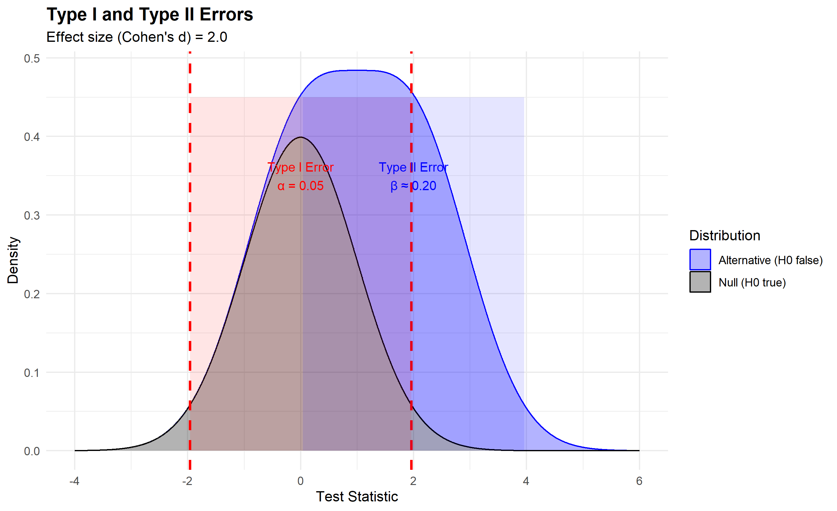
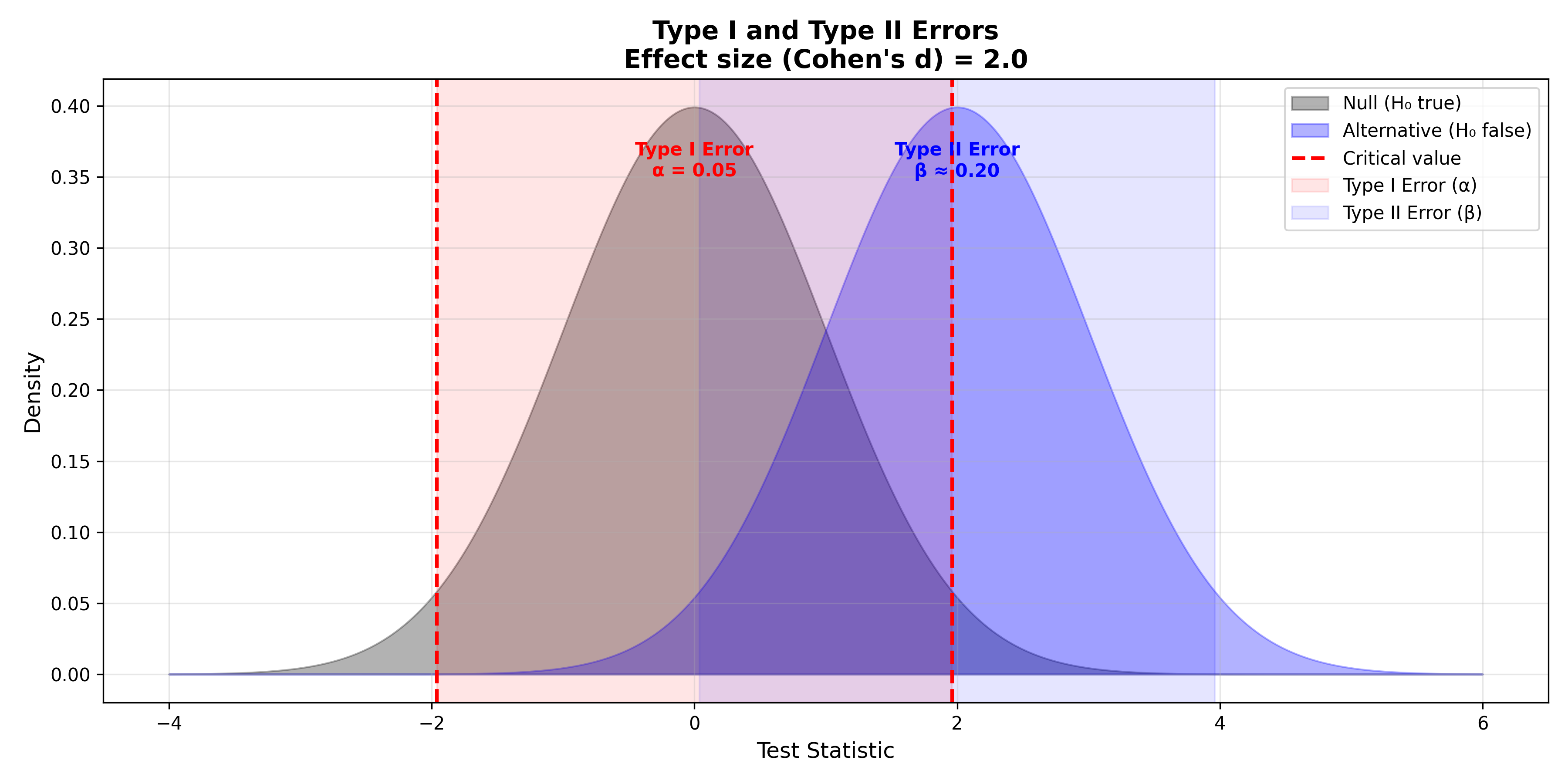
**Type I Error (False Positive, α)**: Rejecting the null when it's actually true. You conclude there's an effect when there isn't. The probability of a Type I error is denoted α (alpha), the significance level. Conventionally, α = 0.05, meaning we tolerate a 5% false positive rate. In the criminal justice analogy, a Type I error is convicting an innocent person—a serious error.
**Type II Error (False Negative, β)**: Failing to reject the null when it's actually false. You conclude there's no effect when there actually is one. The probability of a Type II error is β (beta). If α = 0.05 and β = 0.20 (typical values), then you have an 80% chance of detecting a true effect, called **statistical power** = 1 - β. In the justice system, a Type II error is acquitting a guilty person.
**The Trade-Off**: These errors trade off. To reduce α (fewer false positives), you raise the threshold for rejecting the null, which increases β (more false negatives). You can't minimize both simultaneously with a fixed sample size. The practical choice depends on context. In drug safety testing, you want low α (avoid approving harmful drugs). In early-stage research, you might tolerate higher α (avoid missing promising leads).
**Effect Size**: How large an effect must be to detect it? The **effect size** quantifies the magnitude of the difference. Cohen's d measures standardized difference between two means: $d = \frac{\mu_1 - \mu_2}{\sigma}$. Small effect (d = 0.2), medium (d = 0.5), large (d = 0.8). Larger effects are easier to detect; tiny effects require huge sample sizes.
:::
::: {.callout-tip icon="false"}
## 🔑 Key Formula
**Type I and Type II Errors (Confusion Matrix):**
| | Null True | Null False |
|---|-----------|------------|
| Reject Null | Type I Error (α) | Correct (Power) |
| Fail to Reject | Correct (1 - α) | Type II Error (β) |
**Statistical Power:**
$$\text{Power} = 1 - \beta = P(\text{Reject } H_0 \mid H_0 \text{ is false})$$
**Cohen's d (Effect Size):**
$$d = \frac{\mu_1 - \mu_2}{\sigma}$$
where σ is the pooled standard deviation.
:::
Let's visualize Type I and Type II errors:
::: {.panel-tabset}
## R
```{r}
library(ggplot2)
library(tidyverse)

# Visualize Type I and Type II errors
# Assume two distributions: null (centered at 0) and alternative (centered at effect size)

# Create data
null_dist <- tibble(
  x = seq(-4, 6, length.out = 1000),
  density = dnorm(x, mean = 0, sd = 1),
  group = "Null (H0 true)"
)

effect_size <- 2  # Cohen's d
alt_dist <- tibble(
  x = seq(-4, 6, length.out = 1000),
  density = dnorm(x, mean = effect_size, sd = 1),
  group = "Alternative (H0 false)"
)

combined <- bind_rows(null_dist, alt_dist)

# Critical value (two-tailed, alpha = 0.05)
critical_value <- qnorm(0.975)  # 1.96 for two-tailed alpha=0.05

ggplot(combined, aes(x = x, y = density, color = group, fill = group)) +
  geom_area(alpha = 0.3) +
  geom_vline(xintercept = critical_value, linetype = "dashed", color = "red", linewidth = 1) +
  geom_vline(xintercept = -critical_value, linetype = "dashed", color = "red", linewidth = 1) +
  # Shade Type I error region
  annotate("rect", xmin = -critical_value, xmax = critical_value, ymin = 0, ymax = 0.45,
           alpha = 0.1, fill = "red", label = "Type I Error (α)") +
  # Shade Type II error region
  annotate("rect", xmin = effect_size - critical_value, xmax = effect_size + critical_value,
           ymin = 0, ymax = 0.45, alpha = 0.1, fill = "blue", label = "Type II Error (β)") +
  annotate("text", x = 0, y = 0.35, label = "Type I Error\nα = 0.05", size = 3.5, color = "red") +
  annotate("text", x = 2, y = 0.35, label = "Type II Error\nβ ≈ 0.20", size = 3.5, color = "blue") +
  scale_color_manual(values = c("Null (H0 true)" = "black", "Alternative (H0 false)" = "blue")) +
  scale_fill_manual(values = c("Null (H0 true)" = "black", "Alternative (H0 false)" = "blue")) +
  labs(
    title = "Type I and Type II Errors",
    subtitle = "Effect size (Cohen's d) = 2.0",
    x = "Test Statistic",
    y = "Density",
    color = "Distribution",
    fill = "Distribution"
  ) +
  theme_minimal() +
  theme(
    plot.title = element_text(face = "bold", size = 14),
    legend.position = "right"
  )
```
## Python
```{python}
import numpy as np
import matplotlib.pyplot as plt
from scipy.stats import norm

# Visualize Type I and Type II errors
x = np.linspace(-4, 6, 1000)
null_density = norm.pdf(x, 0, 1)
effect_size = 2.0
alt_density = norm.pdf(x, effect_size, 1)

critical_value = norm.ppf(0.975)  # ~1.96 for two-tailed alpha=0.05

fig, ax = plt.subplots(figsize=(12, 6))

# Plot distributions
ax.fill_between(x, null_density, alpha=0.3, color='black', label='Null (H₀ true)')
ax.fill_between(x, alt_density, alpha=0.3, color='blue', label='Alternative (H₀ false)')

# Critical values
ax.axvline(critical_value, linestyle='--', color='red', linewidth=2, label='Critical value')
ax.axvline(-critical_value, linestyle='--', color='red', linewidth=2)

# Shade error regions
ax.axvspan(-critical_value, critical_value, alpha=0.1, color='red', label='Type I Error (α)')
ax.axvspan(effect_size - critical_value, effect_size + critical_value,
           alpha=0.1, color='blue', label='Type II Error (β)')

# Labels
ax.text(0, 0.35, 'Type I Error\nα = 0.05', ha='center', fontsize=10, color='red', fontweight='bold')
ax.text(effect_size, 0.35, 'Type II Error\nβ ≈ 0.20', ha='center', fontsize=10, color='blue', fontweight='bold')

ax.set_xlabel('Test Statistic', fontsize=12)
ax.set_ylabel('Density', fontsize=12)
ax.set_title('Type I and Type II Errors\nEffect size (Cohen\'s d) = 2.0', fontsize=14, fontweight='bold')
ax.legend(loc='upper right')
ax.grid(alpha=0.3)
plt.tight_layout()
plt.show()
```
:::
::: {.callout-caution icon="false"}
## 📝 Section 6.2 Review Questions
1. What is a Type I error, and in business context, give an example of when you'd want to minimize it.
2. What is a Type II error, and why might you tolerate a higher Type II error rate in exploratory research?
3. Explain the trade-off between Type I and Type II errors. Can you minimize both simultaneously with a fixed sample size?
4. What is statistical power, and how does it relate to sample size and effect size?
5. If Cohen's d = 0.2 (small effect), what implication does this have for the sample size needed to detect it with power = 0.80?
:::
## The p-value Demystified
The p-value is simultaneously one of the most used and most misunderstood concepts in statistics. Let's clarify what it is and—equally important—what it isn't.
::: {.callout-note icon="false"}
## 📘 Theory: The Correct Definition and Common Misconceptions
**The Correct Definition**: The p-value is the probability of observing a test statistic as extreme as (or more extreme than) the one observed, *assuming the null hypothesis is true*. It is a measure of how consistent the data are with the null hypothesis. A small p-value (e.g., 0.02) means that if the null were true, observing such extreme data would be rare—only 2% of the time. This provides evidence against the null.
**What the p-value is NOT:**
1. **Not the probability the null is true.** If p = 0.05, it does not mean there's a 5% chance the null hypothesis is true. The null is either true or false; probability doesn't apply. The p-value conditions on the null being true.
2. **Not the probability the alternative is true.** A small p-value doesn't tell you the probability your hypothesis is correct. It tells you how unlikely the data are if the null is true.
3. **Not a measure of practical significance.** A p-value of 0.001 indicates strong evidence against the null, but the effect might be tiny and irrelevant. Conversely, a p-value of 0.08 might represent a substantial effect you don't want to ignore just because it's not "statistically significant."
**The Replication Crisis**: In recent years, scientists have discovered that p-values and "statistical significance" (p < 0.05) can be misleading at scale. Many published results with p < 0.05 don't replicate. Why? When many studies test many hypotheses and only significant results are published, the bar is accidentally lowered—studies with p = 0.049 get published and celebrated, while p = 0.051 are filed away. This is **publication bias**. Additionally, researchers sometimes "p-hack"—testing many hypotheses until they find significance—which inflates false positives. Modern practice stresses **pre-registration** (committing to analyses before data collection) and **effect sizes** alongside p-values.
:::
::: {.callout-caution icon="false"}
## 📝 Section 6.3 Review Questions
1. State the correct definition of a p-value in one sentence.
2. Why is it incorrect to say "there's a 5% probability the null hypothesis is true" when p = 0.05?
3. Explain the replication crisis and the role of publication bias in inflating false positives.
4. If you test 100 hypotheses at α = 0.05, how many false positives would you expect, even if all nulls are true?
5. Why do modern statisticians recommend reporting effect sizes alongside p-values?
:::
## The t-test Family
The t-test is the most common statistical test, and it comes in three flavors. All assume data are roughly normally distributed and observations are independent.
::: {.callout-note icon="false"}
## 📘 Theory: One-Sample, Independent, and Paired t-Tests
**One-Sample t-Test**: Tests whether the mean of a single sample differs from a hypothesized value (the null hypothesis). Example: "Does average transaction value (μ) equal 50,000 naira?" Null: μ = 50,000. Alternative: μ ≠ 50,000 (two-tailed). The test statistic is:
$$t = \frac{\bar{x} - \mu_0}{SE} = \frac{\bar{x} - \mu_0}{s / \sqrt{n}}$$
where $\bar{x}$ is the sample mean, $\mu_0$ is the hypothesized mean, s is the sample standard deviation, and n is sample size.
**Independent Samples t-Test**: Compares the means of two independent groups. Example: "Do men and women in Lagos earn different average wages?" Null: μ₁ = μ₂. The test statistic depends on whether variances are equal. If equal (which you can test with Levene's test):
$$t = \frac{\bar{x}_1 - \bar{x}_2}{SE_{\text{pooled}}}$$
where $SE_{\text{pooled}} = \sqrt{\frac{s_1^2(n_1 - 1) + s_2^2(n_2 - 1)}{n_1 + n_2 - 2} \left(\frac{1}{n_1} + \frac{1}{n_2}\right)}$. If variances are unequal (Welch's test), the formula is slightly different.
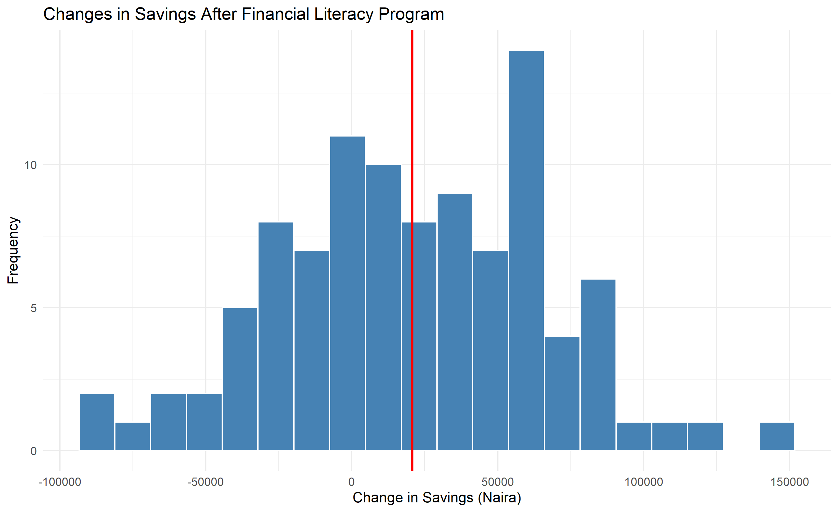
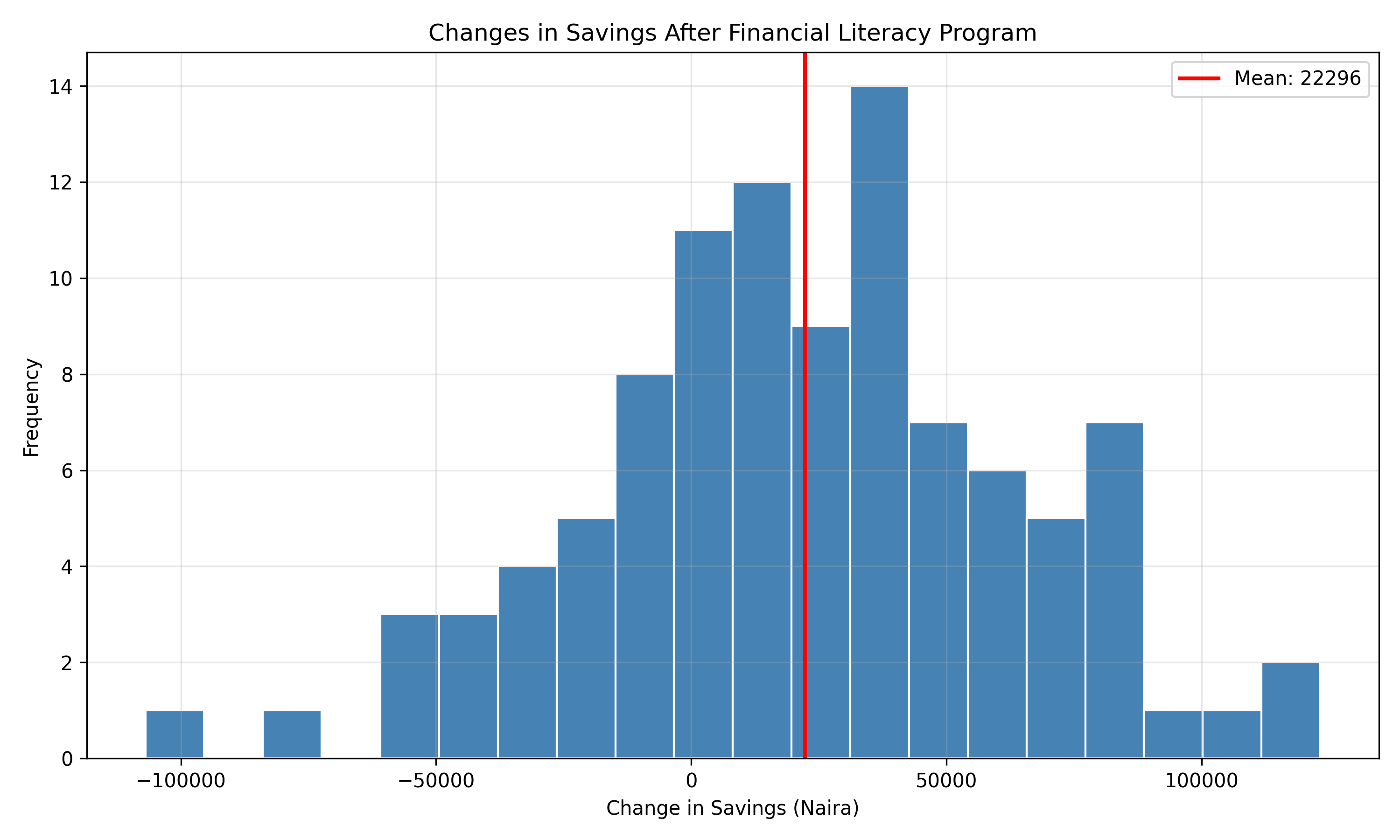
**Paired t-Test**: Compares means of two related measurements (e.g., before and after, left and right). Example: "Does a training program increase average productivity?" Null: μ_difference = 0. The test operates on the differences:
$$t = \frac{\bar{d} - 0}{s_d / \sqrt{n}}$$
where $\bar{d}$ is the mean difference and $s_d$ is its standard deviation.
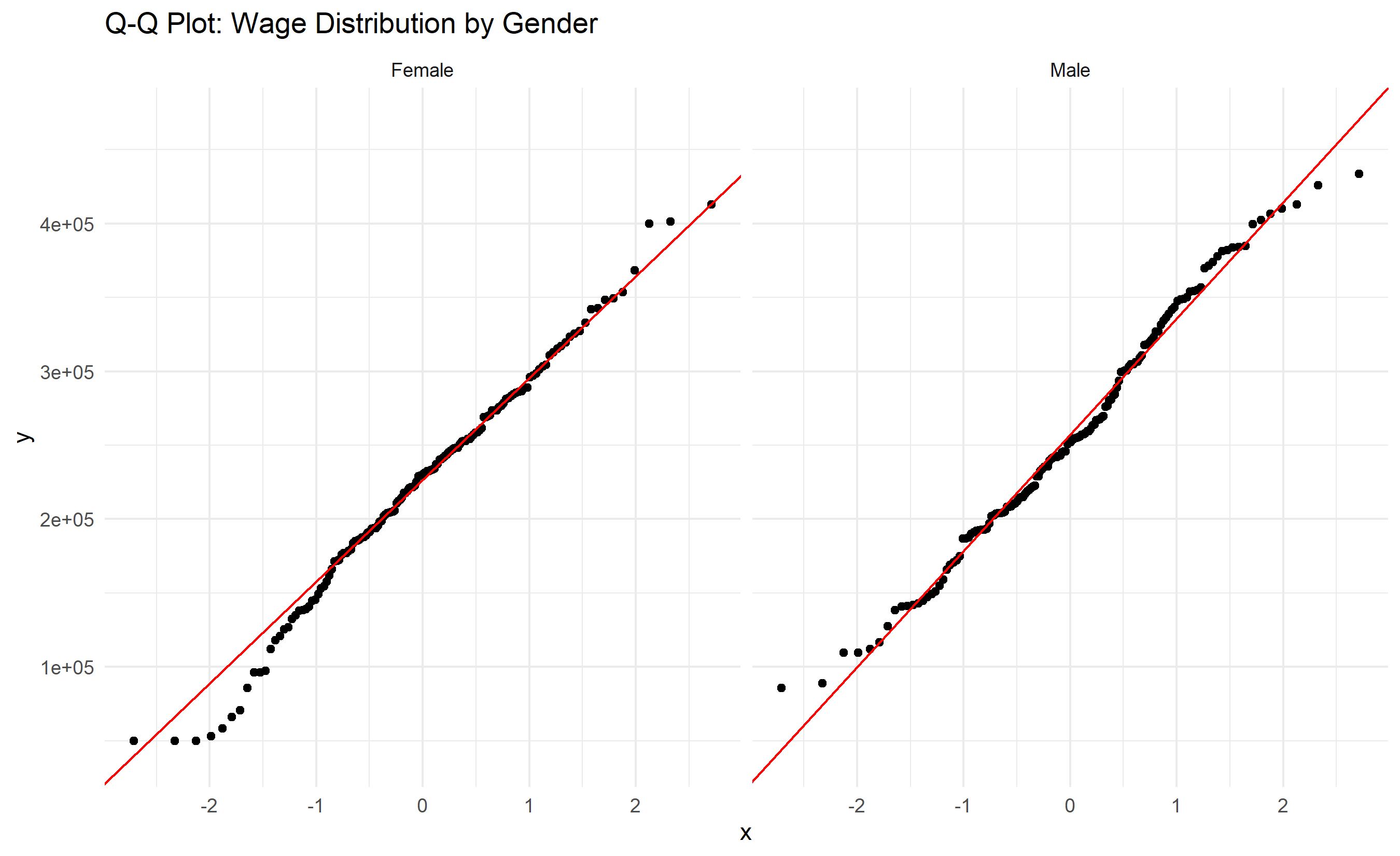
**Assumptions**: All t-tests assume (1) normality of the underlying distribution and (2) independence of observations. For large samples (n > 30), the t-test is robust to mild violations of normality due to the Central Limit Theorem. For small samples, check normality with a Q-Q plot or the Shapiro-Wilk test.
:::
Let's apply t-tests to Nigerian banking data:
::: {.panel-tabset}
## R
```{r}
library(tidyverse)
library(broom)
# Create synthetic Nigerian bank customer data
set.seed(123)
# One-sample test: Does average transaction value differ from 50,000 naira?
transactions <- tibble(
customer_id = 1:200,
amount = rnorm(200, mean = 55000, sd = 25000) |> pmax(1000)
)
# One-sample t-test
t_test_result <- t.test(transactions$amount, mu = 50000)
print(t_test_result)
print(tidy(t_test_result))
# Effect size: Cohen's d
mean_diff <- mean(transactions$amount) - 50000
pooled_sd <- sd(transactions$amount)
cohens_d <- mean_diff / pooled_sd
cat(sprintf("Cohen's d: %.3f\n", cohens_d))
# Independent samples test: Do men and women earn different wages?
wage_data <- tibble(
employee_id = 1:300,
gender = c(rep("Male", 150), rep("Female", 150)),
monthly_wage = c(
rnorm(150, mean = 250000, sd = 80000), # Male wages
rnorm(150, mean = 220000, sd = 75000) # Female wages (lower on average)
) |> pmax(50000)
)
# Check normality (Q-Q plot)
ggplot(wage_data, aes(sample = monthly_wage)) +
stat_qq() +
stat_qq_line(color = "red") +
facet_wrap(~gender) +
labs(title = "Q-Q Plot: Wage Distribution by Gender") +
theme_minimal()
# Independent samples t-test
t_test_wage <- t.test(
filter(wage_data, gender == "Male")$monthly_wage,
filter(wage_data, gender == "Female")$monthly_wage,
var.equal = FALSE # Welch's test (doesn't assume equal variances)
)
print(t_test_wage)
print(tidy(t_test_wage))
# Effect size
male_wage <- filter(wage_data, gender == "Male")$monthly_wage
female_wage <- filter(wage_data, gender == "Female")$monthly_wage
cohens_d_wage <- (mean(male_wage) - mean(female_wage)) /
sqrt(((length(male_wage) - 1) * var(male_wage) +
(length(female_wage) - 1) * var(female_wage)) /
(length(male_wage) + length(female_wage) - 2))
cat(sprintf("\nCohens's d for wage gap: %.3f\n", cohens_d_wage))
# Levene's test for equal variances
car::leveneTest(monthly_wage ~ gender, data = wage_data)
# Paired t-test: Does a financial literacy program improve savings?
literacy_data <- tibble(
participant_id = 1:100,
savings_before = rnorm(100, mean = 50000, sd = 30000) |> pmax(5000),
savings_after = rnorm(100, mean = 75000, sd = 35000) |> pmax(5000)
) |>
mutate(savings_diff = savings_after - savings_before)
t_test_paired <- t.test(
literacy_data$savings_after,
literacy_data$savings_before,
paired = TRUE
)
print(t_test_paired)
print(tidy(t_test_paired))
# Visualize the paired differences
ggplot(literacy_data, aes(x = savings_diff)) +
geom_histogram(bins = 20, fill = "steelblue", color = "white") +
geom_vline(aes(xintercept = mean(savings_diff)), color = "red", linewidth = 1) +
labs(
title = "Changes in Savings After Financial Literacy Program",
x = "Change in Savings (Naira)",
y = "Frequency"
) +
theme_minimal()
# Summary table
summary_table <- tribble(
~Test, ~Null.Hypothesis, ~p.value, ~Effect.Size, ~Interpretation,
"One-sample", "Transaction = 50,000 naira", round(t_test_result$p.value, 4),
round(cohens_d, 3), "Reject null; actual > 50,000",
"Independent", "Male wage = Female wage", round(t_test_wage$p.value, 4),
round(cohens_d_wage, 3), "Reject null; gender wage gap exists",
"Paired", "Savings change = 0", round(t_test_paired$p.value, 4),
round(mean(literacy_data$savings_diff) / sd(literacy_data$savings_diff), 3),
"Reject null; program increases savings"
)
print(summary_table)
```
## Python
```{python}
import numpy as np
from scipy import stats
import pandas as pd
import matplotlib.pyplot as plt
# One-sample t-test
np.random.seed(123)
transactions = np.random.normal(55000, 25000, 200)
transactions = np.maximum(transactions, 1000)
t_stat, p_val = stats.ttest_1samp(transactions, 50000)
print("ONE-SAMPLE T-TEST")
print(f"t-statistic: {t_stat:.4f}")
print(f"p-value: {p_val:.4f}")
print(f"Mean transaction: {transactions.mean():.2f} naira")
# Cohen's d
cohens_d = (transactions.mean() - 50000) / transactions.std()
print(f"Cohen's d: {cohens_d:.3f}\n")
# Independent samples t-test
male_wages = np.maximum(np.random.normal(250000, 80000, 150), 50000)
female_wages = np.maximum(np.random.normal(220000, 75000, 150), 50000)
t_stat_wage, p_val_wage = stats.ttest_ind(male_wages, female_wages, equal_var=False)
print("INDEPENDENT SAMPLES T-TEST")
print(f"t-statistic: {t_stat_wage:.4f}")
print(f"p-value: {p_val_wage:.4f}")
print(f"Mean male wage: {male_wages.mean():.2f} naira")
print(f"Mean female wage: {female_wages.mean():.2f} naira")
# Cohen's d
cohens_d_wage = (male_wages.mean() - female_wages.mean()) / \
np.sqrt(((len(male_wages) - 1) * male_wages.var() +
(len(female_wages) - 1) * female_wages.var()) / \
(len(male_wages) + len(female_wages) - 2))
print(f"Cohen's d: {cohens_d_wage:.3f}\n")
# Levene's test for equal variances
stat_levene, p_levene = stats.levene(male_wages, female_wages)
print(f"Levene's test p-value: {p_levene:.4f}")
print(f"Equal variances: {'Yes' if p_levene > 0.05 else 'No'}\n")
# Paired t-test
savings_before = np.maximum(np.random.normal(50000, 30000, 100), 5000)
savings_after = np.maximum(np.random.normal(75000, 35000, 100), 5000)
savings_diff = savings_after - savings_before
t_stat_paired, p_val_paired = stats.ttest_rel(savings_after, savings_before)
print("PAIRED T-TEST")
print(f"t-statistic: {t_stat_paired:.4f}")
print(f"p-value: {p_val_paired:.4f}")
print(f"Mean change in savings: {savings_diff.mean():.2f} naira")
# Visualize paired differences
plt.figure(figsize=(10, 6))
plt.hist(savings_diff, bins=20, color='steelblue', edgecolor='white')
plt.axvline(savings_diff.mean(), color='red', linewidth=2, label=f'Mean: {savings_diff.mean():.0f}')
plt.xlabel('Change in Savings (Naira)')
plt.ylabel('Frequency')
plt.title('Changes in Savings After Financial Literacy Program')
plt.legend()
plt.grid(alpha=0.3)
plt.tight_layout()
plt.show()
# Summary table
summary_df = pd.DataFrame({
'Test': ['One-sample', 'Independent', 'Paired'],
'Null Hypothesis': ['Trans = 50,000', 'Male = Female', 'Change = 0'],
'p-value': [p_val, p_val_wage, p_val_paired],
'Effect Size (d)': [cohens_d, cohens_d_wage,
savings_diff.mean() / savings_diff.std()],
'Interpretation': ['Reject; actual > 50k', 'Reject; wage gap',
'Reject; savings increase']
})
print("\nSUMMARY TABLE")
print(summary_df.to_string(index=False))
```
:::
::: {.callout-caution icon="false"}
## 📝 Section 6.4 Review Questions
1. When would you use a paired t-test vs. an independent samples t-test? Give a business example for each.
2. What is Levene's test, and when should you consult its result?
3. Explain the relationship between sample size, effect size, and statistical power in the context of t-tests.
4. If a one-sample t-test yields p = 0.06, should you conclude the null is true? Explain.
5. How do you interpret Cohen's d = 0.4? What does this tell you about the practical significance?
:::
## The Chi-Squared Test
When your data are categorical, the chi-squared test assesses whether two categorical variables are independent.
::: {.callout-note icon="false"}
## 📘 Theory: Contingency Tables and the Chi-Squared Statistic
A **contingency table** (or crosstabulation) shows the joint distribution of two categorical variables. Example: In a bank, you have loan applicants classified by employment status (employed, self-employed, unemployed) and loan default (yes, no). The contingency table counts how many fall into each cell.
The **chi-squared test** compares observed counts (O) to expected counts (E) under independence. If the variables are independent, the expected count in each cell is:
$$E_{ij} = \frac{(\text{Row } i \text{ total}) \times (\text{Column } j \text{ total})}{\text{Grand Total}}$$
The chi-squared statistic is:
$$\chi^2 = \sum \frac{(O - E)^2}{E}$$
If observed counts deviate substantially from expected counts, χ² is large, indicating dependence. The p-value is computed from the chi-squared distribution with degrees of freedom = (rows - 1) × (columns - 1).
**Cramér's V** measures the strength of association:
$$V = \sqrt{\frac{\chi^2}{n(k - 1)}}$$
where n is the sample size and k is the minimum of (rows, columns). V ranges from 0 (no association) to 1 (perfect association).
**Assumptions**: Each cell should have at least 5 expected counts. If this is violated, use **Fisher's exact test** (for 2×2 tables) or simulate p-values.
:::
::: {.panel-tabset}
## R
```{r}
# Chi-squared test: Are loan defaults independent of employment status?
loan_data <- tibble(
employment = c(rep("Employed", 300), rep("Self-Employed", 150),
rep("Unemployed", 50)),
default = c(
rep(c("No", "Yes"), times = c(280, 20)), # Employed: 20/300 default
rep(c("No", "Yes"), times = c(135, 15)), # Self-employed: 15/150 default
rep(c("No", "Yes"), times = c(35, 15)) # Unemployed: 15/50 default
)
)
# Create contingency table
contingency_table <- table(loan_data$employment, loan_data$default)
print(contingency_table)
# Chi-squared test
chi_test <- chisq.test(contingency_table)
print(chi_test)
# Cramer's V
n <- nrow(loan_data)
cramers_v <- sqrt(chi_test$statistic / (n * (min(dim(contingency_table)) - 1)))
cat(sprintf("Cramér's V: %.3f\n", cramers_v))
# Visualize the contingency table
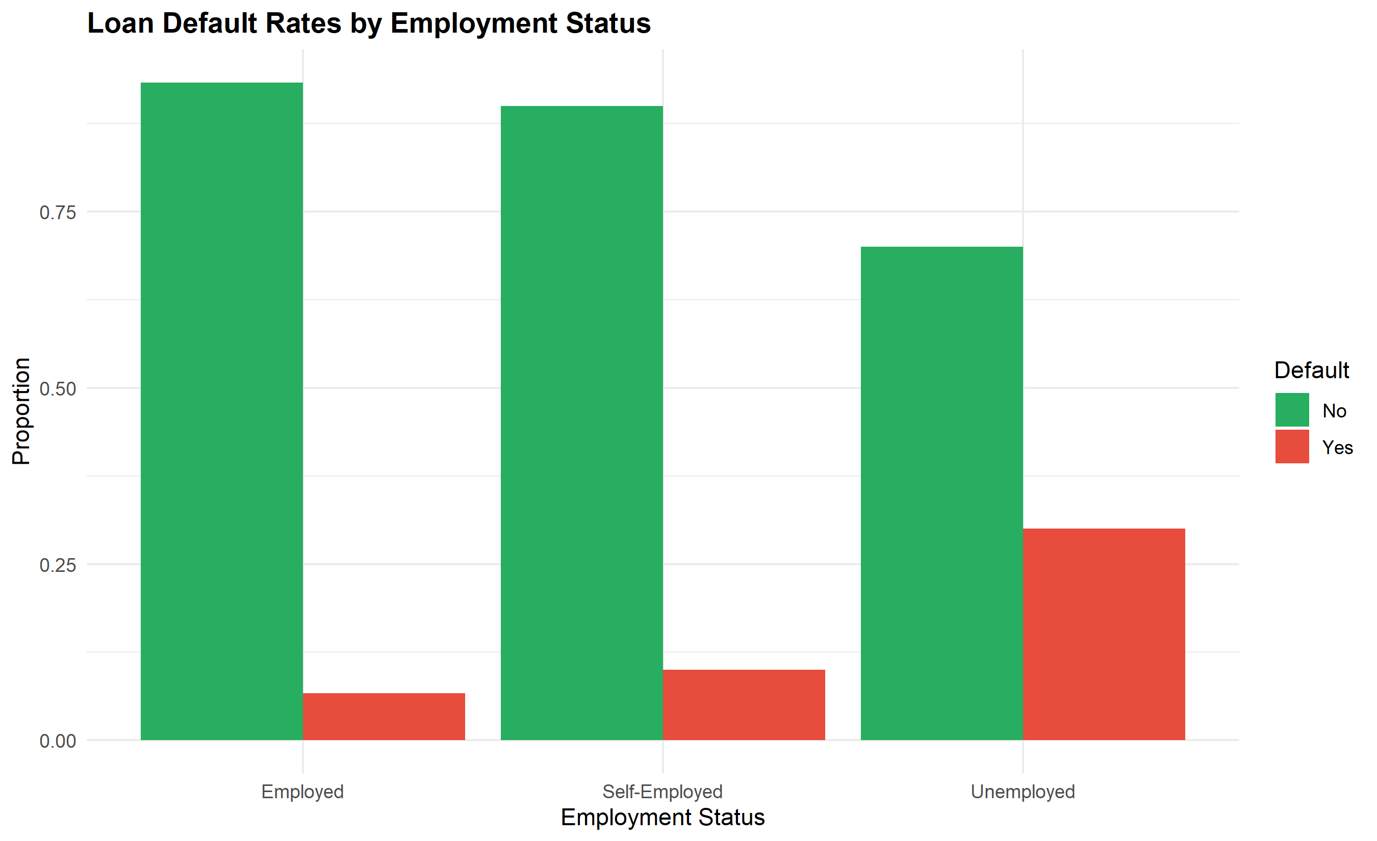
contingency_prop <- prop.table(contingency_table, margin = 1) # Row proportions
contingency_df <- as.data.frame(contingency_prop) |>
rename(Employment = Var1, Default = Var2)
ggplot(contingency_df, aes(x = Employment, y = Freq, fill = Default)) +
geom_col(position = "dodge") +
scale_fill_manual(values = c("No" = "#27AE60", "Yes" = "#E74C3C")) +
labs(
title = "Loan Default Rates by Employment Status",
x = "Employment Status",
y = "Proportion",
fill = "Default"
) +
theme_minimal() +
theme(plot.title = element_text(face = "bold"))
# Expected vs. observed counts
expected_counts <- chi_test$expected |>
as.data.frame() |>
rename(Expected_No = No, Expected_Yes = Yes)
observed_counts <- as.data.frame(contingency_table) |>
rename(Employment = Var1, Default = Var2)
cat("\n--- Expected Counts (under independence) ---\n")
print(chi_test$expected)
# Fisher's exact test for small samples
# (chi-squared may not be appropriate if expected < 5)
cat("\n--- Fisher's Exact Test (alternative for small samples) ---\n")
fisher_test <- fisher.test(contingency_table)
print(fisher_test)
```
## Python
```{python}
from scipy.stats import chi2_contingency
import pandas as pd
# Create contingency table
contingency = np.array([
[280, 20], # Employed: 280 no default, 20 default
[135, 15], # Self-employed
[35, 15] # Unemployed
])
# Chi-squared test
chi2, p_val, dof, expected = chi2_contingency(contingency)
print("CHI-SQUARED TEST")
print(f"Chi-squared statistic: {chi2:.4f}")
print(f"p-value: {p_val:.4f}")
print(f"Degrees of freedom: {dof}")
print(f"\nExpected counts:\n{expected}")
# Cramér's V
n = contingency.sum()
k = min(contingency.shape)
cramers_v = np.sqrt(chi2 / (n * (k - 1)))
print(f"\nCramér's V: {cramers_v:.3f}")
# Create DataFrame for visualization
employment = ['Employed', 'Self-Employed', 'Unemployed']
default_no = [280, 135, 35]
default_yes = [20, 15, 15]
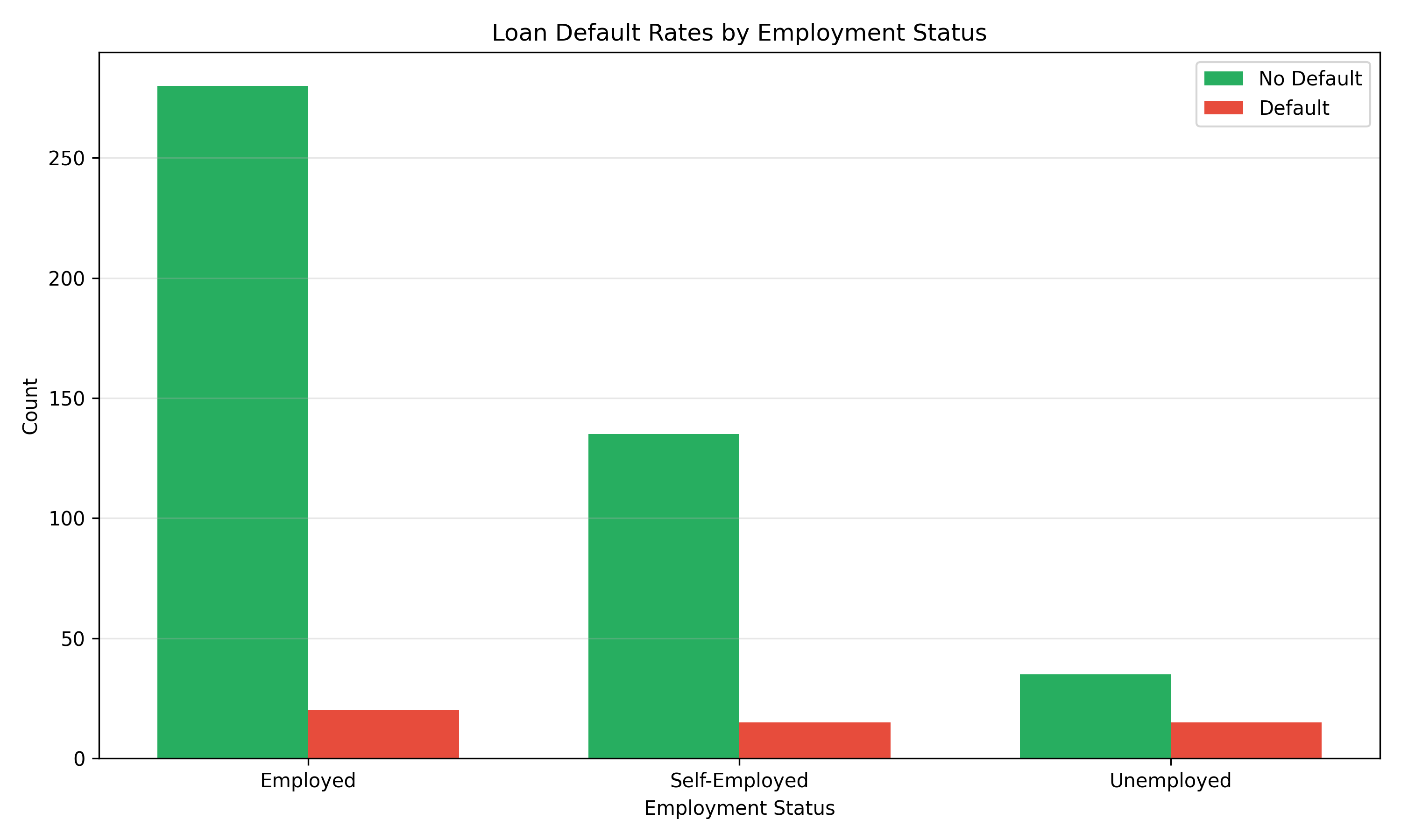
fig, ax = plt.subplots(figsize=(10, 6))
x = np.arange(len(employment))
width = 0.35
ax.bar(x - width/2, default_no, width, label='No Default', color='#27AE60')
ax.bar(x + width/2, default_yes, width, label='Default', color='#E74C3C')
ax.set_xlabel('Employment Status')
ax.set_ylabel('Count')
ax.set_title('Loan Default Rates by Employment Status')
ax.set_xticks(x)
ax.set_xticklabels(employment)
ax.legend()
ax.grid(axis='y', alpha=0.3)
plt.tight_layout()
plt.show()
# Calculate proportions
print("\n--- Default Rates by Employment Status ---")
for i, emp in enumerate(employment):
default_rate = 100 * default_yes[i] / (default_no[i] + default_yes[i])
print(f"{emp}: {default_rate:.1f}%")
```
:::
::: {.callout-caution icon="false"}
## 📝 Section 6.5 Review Questions
1. What is a contingency table, and how does it relate to the chi-squared test?
2. Explain the intuition behind the chi-squared test: what does it compare?
3. When should you use Fisher's exact test instead of chi-squared?
4. What does Cramér's V = 0.2 tell you about the strength of association?
5. In the loan default example, how would you interpret the finding that employment status and default are dependent?
:::
## ANOVA: Comparing More Than Two Groups
When you have three or more groups to compare, ANOVA (Analysis of Variance) extends the t-test framework.
::: {.callout-note icon="false"}
## 📘 Theory: One-Way ANOVA and the F-Statistic
**One-Way ANOVA** tests whether the means of k groups are equal. Null: μ₁ = μ₂ = ... = μ_k. The test compares the variance *between* groups to the variance *within* groups. If groups have different means, between-group variance is large. If all groups have the same mean, between and within variance are similar.
The **F-statistic** is:
$$F = \frac{\text{Between-Group Variance}}{\text{Within-Group Variance}} = \frac{\text{MS}_B}{\text{MS}_W}$$
where MS = Mean Square. Large F indicates group means differ significantly. The p-value is computed from the F-distribution with degrees of freedom df₁ = k - 1 (groups) and df₂ = n - k (observations minus groups).
**Post-Hoc Tests**: If ANOVA rejects the null (p < 0.05), you know *some* groups differ, but not which ones. Use **Tukey's HSD (Honestly Significant Difference)** test to compare all pairs of groups while controlling the false positive rate. Alternatively, use **Bonferroni correction** (divide α by the number of comparisons) for a more conservative approach.
**Two-Way ANOVA** includes two grouping variables, allowing you to test main effects and interactions.
**Assumptions**: Normality within groups, homogeneity of variance (Levene's test), and independence.
:::
::: {.panel-tabset}
## R
```{r}
# One-way ANOVA: Does average loan amount differ across geopolitical zones?

loan_zones <- tibble(
  zone = rep(c("North-West", "North-Central", "South-West", "South-East"), each = 100),
  loan_amount = c(
    rnorm(100, mean = 3000000, sd = 1000000),   # North-West
    rnorm(100, mean = 2500000, sd = 1200000),   # North-Central
    rnorm(100, mean = 4000000, sd = 800000),    # South-West
    rnorm(100, mean = 3500000, sd = 1100000)    # South-East
  ) |> pmax(500000)
)

# Descriptive statistics by zone
loan_zones |>
  group_by(zone) |>
  summarise(
    mean = mean(loan_amount),
    sd = sd(loan_amount),
    n = n(),
    .groups = "drop"
  ) |>
  arrange(desc(mean))
# Check assumptions: Levene's test (equal variances)
car::leveneTest(loan_amount ~ zone, data = loan_zones)
# One-way ANOVA
anova_result <- aov(loan_amount ~ zone, data = loan_zones)
summary(anova_result)
# Effect size: Eta-squared
ss_between <- sum(residuals(anova_result, type = "response")^2)
ss_total <- sum((loan_zones$loan_amount - mean(loan_zones$loan_amount))^2)
eta_squared <- 1 - (ss_between / ss_total)
# Better calculation:
anova_table <- anova(anova_result)
ss_total <- sum(anova_table$`Sum Sq`)
ss_between <- anova_table$`Sum Sq`[1]
eta_squared <- ss_between / ss_total
cat(sprintf("Eta-squared (effect size): %.3f\n", eta_squared))
# Post-hoc test: Tukey HSD
tukey_result <- TukeyHSD(anova_result)
print(tukey_result)
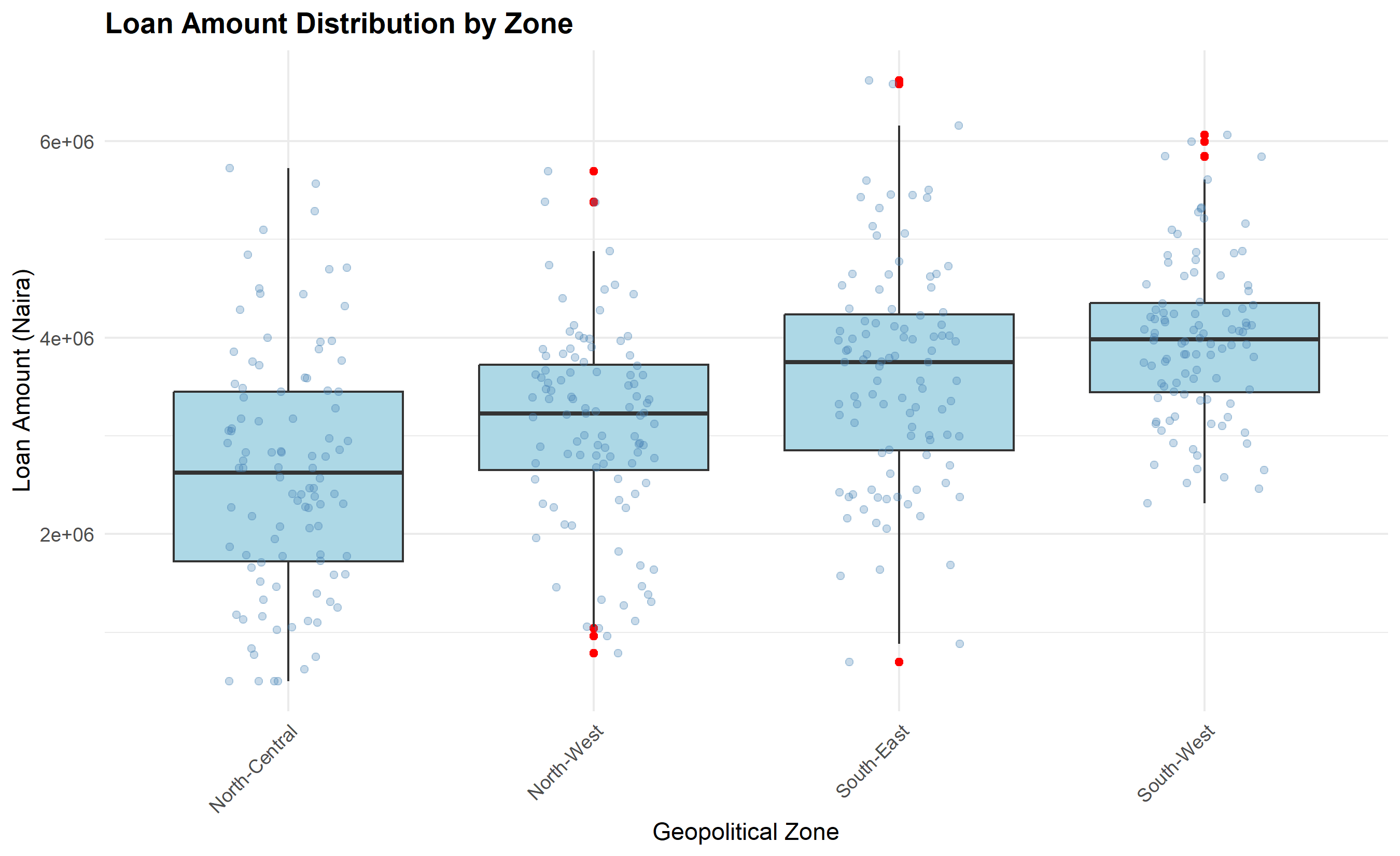
# Visualize with boxplot
ggplot(loan_zones, aes(x = reorder(zone, loan_amount, median), y = loan_amount)) +
geom_boxplot(fill = "lightblue", outlier.colour = "red") +
geom_jitter(width = 0.2, alpha = 0.3, color = "steelblue") +
labs(
title = "Loan Amount Distribution by Zone",
x = "Geopolitical Zone",
y = "Loan Amount (Naira)"
) +
theme_minimal() +
theme(
plot.title = element_text(face = "bold"),
axis.text.x = element_text(angle = 45, hjust = 1)
)
# Two-way ANOVA: Does loan amount differ by zone AND employment status?
loan_zones_2way <- loan_zones |>
mutate(
employment = sample(c("Employed", "Self-Employed", "Unemployed"), n(), replace = TRUE),
loan_amount = loan_amount + ifelse(employment == "Employed", 500000, 0)
)
anova_2way <- aov(loan_amount ~ zone + employment + zone:employment,
data = loan_zones_2way)
summary(anova_2way)
# Visualization: interaction plot
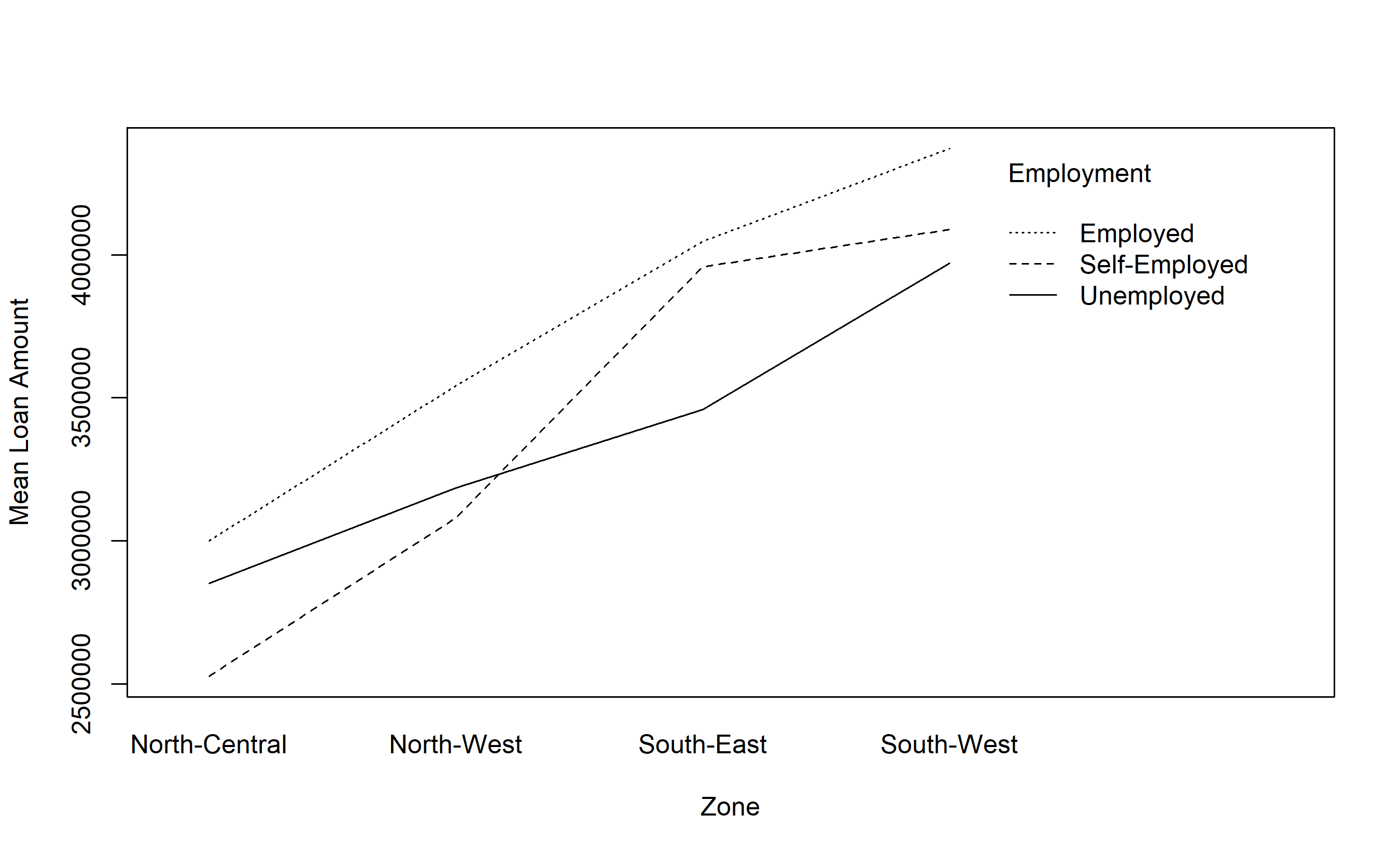
interaction.plot(loan_zones_2way$zone, loan_zones_2way$employment,
loan_zones_2way$loan_amount,
legend = TRUE, xlab = "Zone", ylab = "Mean Loan Amount",
trace.label = "Employment")
```
## Python
```{python}
from scipy.stats import f_oneway
from itertools import combinations
# One-way ANOVA data
np.random.seed(123)
nw_loans = np.maximum(np.random.normal(3000000, 1000000, 100), 500000)
nc_loans = np.maximum(np.random.normal(2500000, 1200000, 100), 500000)
sw_loans = np.maximum(np.random.normal(4000000, 800000, 100), 500000)
se_loans = np.maximum(np.random.normal(3500000, 1100000, 100), 500000)
# One-way ANOVA
f_stat, p_val = f_oneway(nw_loans, nc_loans, sw_loans, se_loans)
print("ONE-WAY ANOVA")
print(f"F-statistic: {f_stat:.4f}")
print(f"p-value: {p_val:.6f}")
# Descriptive statistics
zones_list = ["North-West", "North-Central", "South-West", "South-East"]
loan_lists = [nw_loans, nc_loans, sw_loans, se_loans]
for zone, loans in zip(zones_list, loan_lists):
print(f"{zone}: mean = {loans.mean():,.0f}, sd = {loans.std():,.0f}")
# Effect size: Eta-squared
grand_mean = np.concatenate([nw_loans, nc_loans, sw_loans, se_loans]).mean()
ss_between = sum(len(loans) * (loans.mean() - grand_mean)**2
for loans in loan_lists)
ss_total = sum((x - grand_mean)**2 for loans in loan_lists for x in loans)
eta_squared = ss_between / ss_total
print(f"\nEta-squared (effect size): {eta_squared:.3f}")
# Pairwise comparisons (Bonferroni correction)
from scipy.stats import ttest_ind
n_comparisons = len(list(combinations(range(4), 2)))
bonferroni_alpha = 0.05 / n_comparisons
print(f"\nPAIRWISE COMPARISONS (Bonferroni α = {bonferroni_alpha:.4f}):")
for (i, j) in combinations(range(4), 2):
t_stat, p = ttest_ind(loan_lists[i], loan_lists[j], equal_var=False)
sig = "***" if p < bonferroni_alpha else ""
print(f"{zones_list[i]} vs {zones_list[j]}: p = {p:.6f} {sig}")
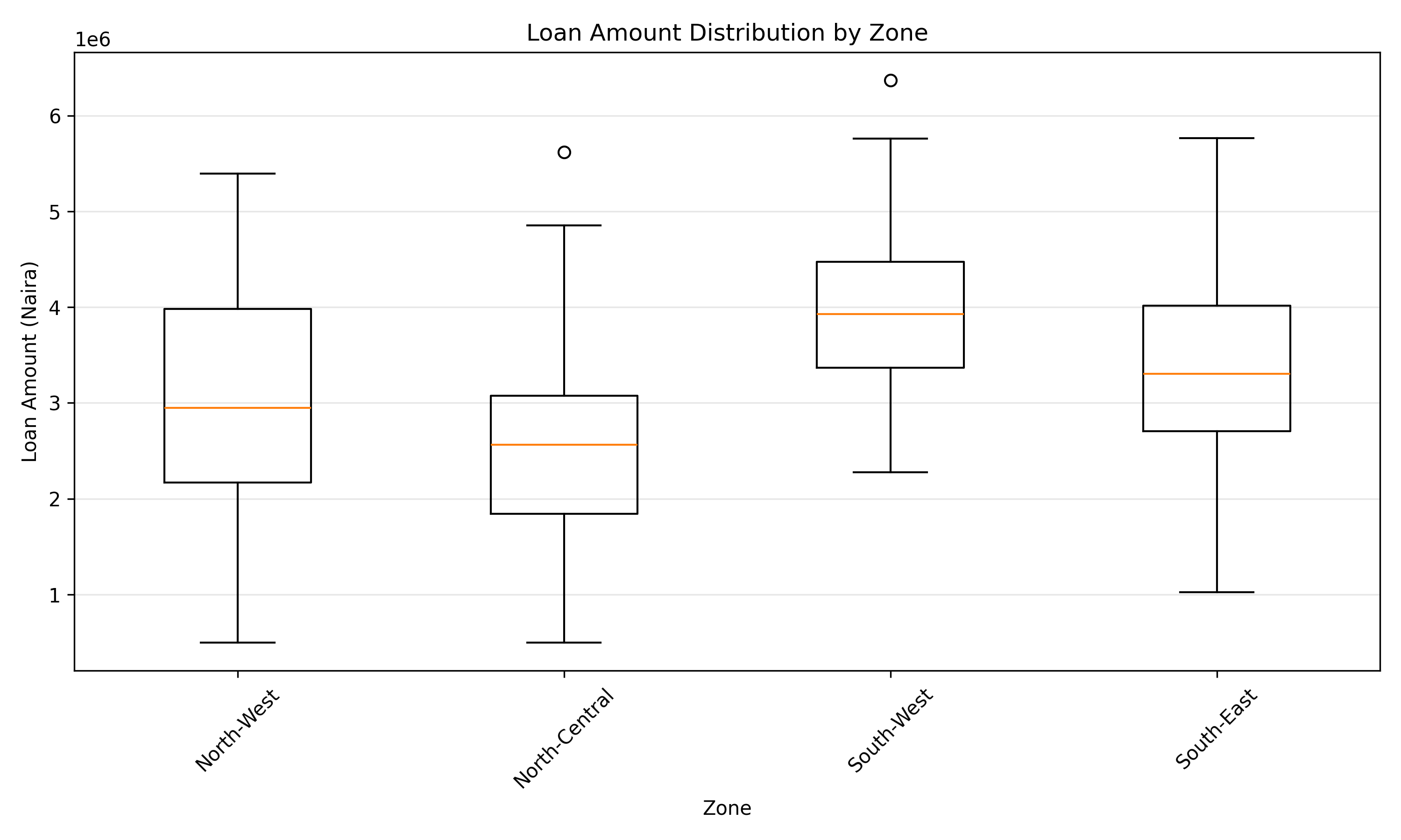
# Boxplot
fig, ax = plt.subplots(figsize=(10, 6))
ax.boxplot([nw_loans, nc_loans, sw_loans, se_loans], labels=zones_list)
ax.set_ylabel('Loan Amount (Naira)')
ax.set_xlabel('Zone')
ax.set_title('Loan Amount Distribution by Zone')
ax.grid(alpha=0.3, axis='y')
plt.xticks(rotation=45)
plt.tight_layout()
plt.show()
```
:::
::: {.callout-caution icon="false"}
## 📝 Section 6.6 Review Questions
1. How does ANOVA extend the t-test for comparing more than two groups?
2. What is the intuition behind the F-statistic in ANOVA?
3. Why do you need post-hoc tests like Tukey HSD after rejecting the null in ANOVA?
4. What is the Bonferroni correction, and why is it conservative?
5. Explain the difference between main effects and interactions in two-way ANOVA.
:::
## Non-Parametric Alternatives
When normality fails or data are ordinal (ranked), non-parametric tests don't assume a distribution.
::: {.callout-note icon="false"}
## 📘 Theory: Distribution-Free Methods
**Mann-Whitney U Test** (non-parametric alternative to independent t-test): Tests whether two groups have the same distribution by comparing ranks. It's more robust to outliers than the t-test.
**Kruskal-Wallis Test** (non-parametric ANOVA): Tests whether k groups have the same distribution.
**Wilcoxon Signed-Rank Test** (non-parametric paired t-test): Tests paired data without assuming normality.
**Spearman Rank Correlation**: Measures association between two variables using ranks, robust to outliers and non-linear relationships.
Use these when (1) sample size is small and normality is questionable, (2) data are ordinal (e.g., survey ratings 1–5), or (3) outliers are present.
:::
::: {.panel-tabset}
## R
```{r}
# Non-parametric tests

# Mann-Whitney U: Do casual and formal employees earn differently?
casual_wage <- rnorm(50, mean = 100000, sd = 40000) |> pmax(10000)
formal_wage <- rnorm(50, mean = 150000, sd = 50000) |> pmax(10000)

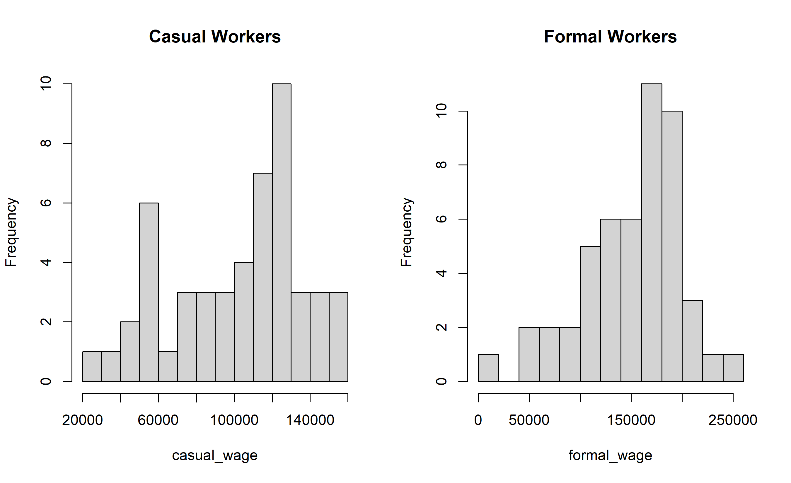
# Distribution check
par(mfrow = c(1, 2))
hist(casual_wage, main = "Casual Workers", breaks = 15)
hist(formal_wage, main = "Formal Workers", breaks = 15)
par(mfrow = c(1, 1))
# Mann-Whitney U test
mw_test <- wilcox.test(casual_wage, formal_wage)
print(mw_test)
# Kruskal-Wallis: Do three income groups differ in spending?
spending_data <- tibble(
group = rep(c("Low", "Medium", "High"), each = 50),
spending = c(
rnorm(50, mean = 20000, sd = 10000) |> pmax(1000),
rnorm(50, mean = 50000, sd = 20000) |> pmax(1000),
rnorm(50, mean = 100000, sd = 30000) |> pmax(1000)
)
)
kw_test <- kruskal.test(spending ~ group, data = spending_data)
print(kw_test)
# Spearman rank correlation: Relationship between education (ordinal) and income
education_level <- c(
rep(1, 30), # Primary
rep(2, 40), # Secondary
rep(3, 50), # Tertiary
rep(4, 30) # Postgraduate
)
income <- c(
rnorm(30, 50000, 20000),
rnorm(40, 150000, 40000),
rnorm(50, 300000, 80000),
rnorm(30, 450000, 100000)
) |> pmax(10000)
spearman_test <- cor.test(education_level, income, method = "spearman")
print(spearman_test)
cat(sprintf("Spearman's rho: %.3f, p-value: %.4f\n",
spearman_test$estimate, spearman_test$p.value))
```
## Python
```{python}
from scipy.stats import mannwhitneyu, kruskal, spearmanr
# Mann-Whitney U test
casual_wage = np.maximum(np.random.normal(100000, 40000, 50), 10000)
formal_wage = np.maximum(np.random.normal(150000, 50000, 50), 10000)
u_stat, p_val = mannwhitneyu(casual_wage, formal_wage)
print("MANN-WHITNEY U TEST")
print(f"U-statistic: {u_stat:.2f}")
print(f"p-value: {p_val:.6f}")
# Kruskal-Wallis test
low_spending = np.maximum(np.random.normal(20000, 10000, 50), 1000)
med_spending = np.maximum(np.random.normal(50000, 20000, 50), 1000)
high_spending = np.maximum(np.random.normal(100000, 30000, 50), 1000)
h_stat, p_val_kw = kruskal(low_spending, med_spending, high_spending)
print("\nKRUSKAL-WALLIS TEST")
print(f"H-statistic: {h_stat:.4f}")
print(f"p-value: {p_val_kw:.6f}")
# Spearman rank correlation
education_level = np.concatenate([
np.repeat(1, 30),
np.repeat(2, 40),
np.repeat(3, 50),
np.repeat(4, 30)
])
income = np.concatenate([
np.maximum(np.random.normal(50000, 20000, 30), 10000),
np.maximum(np.random.normal(150000, 40000, 40), 10000),
np.maximum(np.random.normal(300000, 80000, 50), 10000),
np.maximum(np.random.normal(450000, 100000, 30), 10000)
])
rho, p_spearman = spearmanr(education_level, income)
print("\nSPEARMAN RANK CORRELATION")
print(f"Spearman's rho: {rho:.3f}")
print(f"p-value: {p_spearman:.6f}")
```
:::
::: {.callout-caution icon="false"}
## 📝 Section 6.7 Review Questions
1. When would you choose Mann-Whitney U over an independent samples t-test?
2. What is the advantage of Spearman rank correlation for non-normal data?
3. How do non-parametric tests handle outliers differently than parametric tests?
4. Explain the Kruskal-Wallis test and how it differs from one-way ANOVA.
5. If your data are ordinal (e.g., customer satisfaction 1–5), which test should you use?
:::
## Multiple Comparisons
When you run many statistical tests, the false positive rate accumulates. This is the **multiple comparisons problem**.
::: {.callout-note icon="false"}
## 📘 Theory: Correcting for Multiple Tests
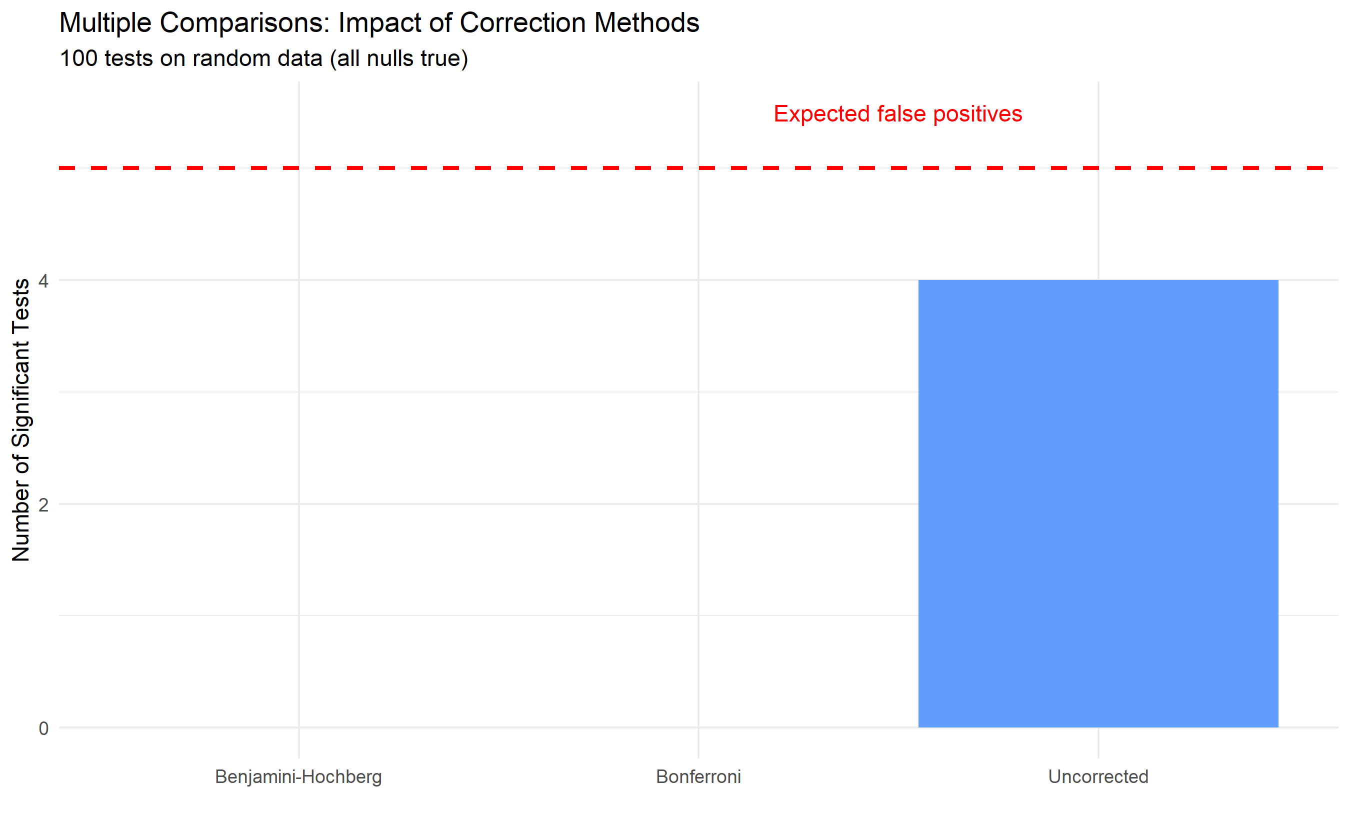
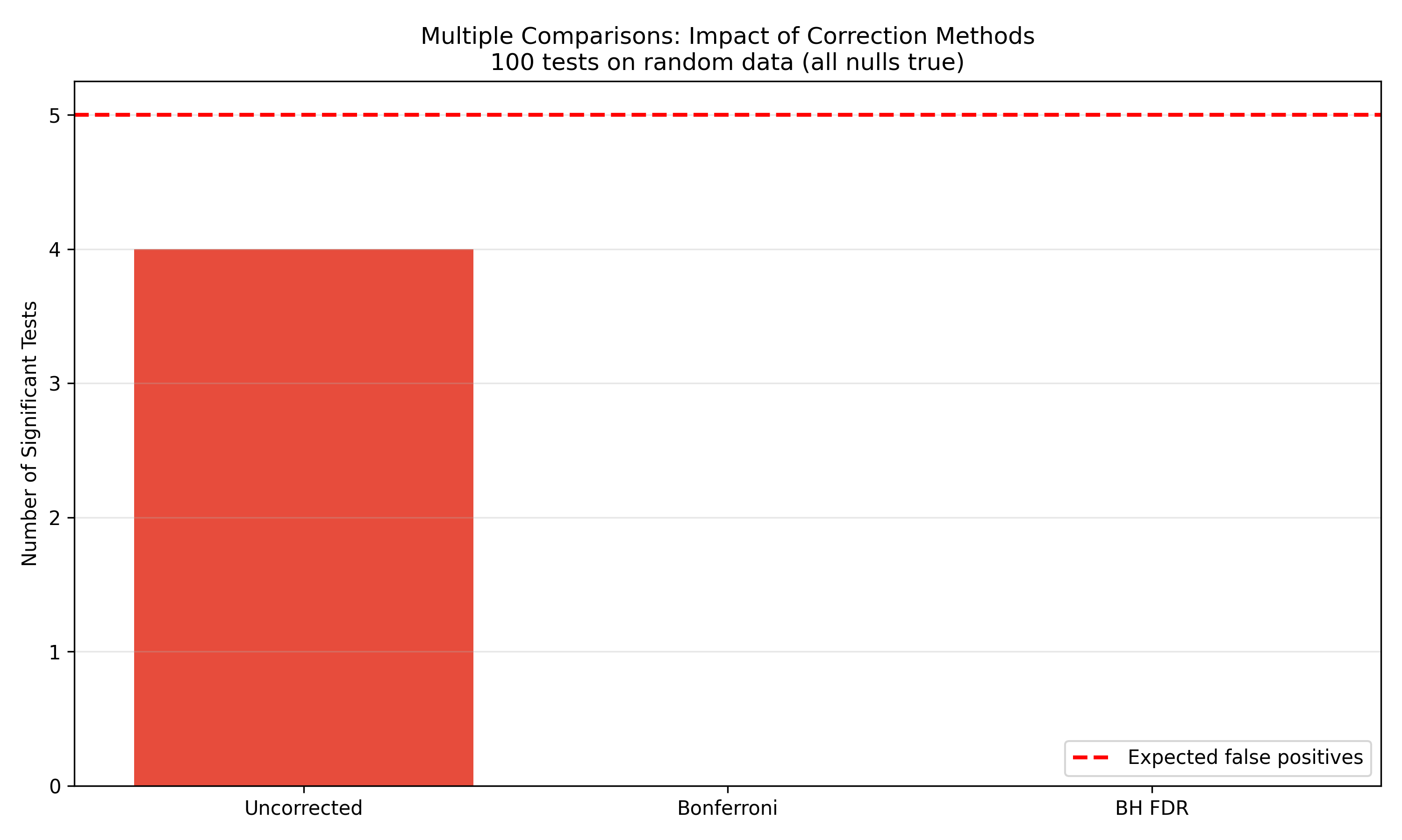
If you test 100 hypotheses at α = 0.05, and all nulls are true, you expect 5 false positives (5% of 100). This inflates the **family-wise error rate** (the probability of at least one false positive across all tests). Several methods correct for this:
1. **Bonferroni Correction**: Divide α by the number of tests. If m tests, use α' = α / m. Conservative but simple. Example: 20 tests, use α = 0.0025 instead of 0.05.
2. **Benjamini-Hochberg FDR Control**: Controls the **False Discovery Rate** (proportion of false positives among all rejections), not the family-wise rate. Less conservative than Bonferroni. Order p-values from smallest to largest. Reject null for test i if p_i ≤ (i / m) × (α / 2).
3. **Tukey Correction**: When comparing pairs in ANOVA, use Tukey HSD instead of multiple t-tests.
**Practical Guidance**: Pre-register your primary hypothesis before data analysis. Distinguish primary tests (critical for your conclusion) from exploratory tests (hypothesis-generating). Apply corrections to exploratory tests.
:::
::: {.panel-tabset}
## R
```{r}
# Demonstration: Multiple comparisons and correction
# Simulate 100 tests on random data (all nulls true)
set.seed(42)
n_tests <- 100L
p_values <- replicate(n_tests, {
x <- rnorm(50)
y <- rnorm(50)
t.test(x, y)$p.value
})
# Uncorrected false positives
uncorrected_sig <- sum(p_values < 0.05)
cat(sprintf("Uncorrected significant tests: %d / %d (expected ~5)\n",
uncorrected_sig, n_tests))
# Bonferroni correction
bonferroni_alpha <- 0.05 / n_tests
bonferroni_sig <- sum(p_values < bonferroni_alpha)
cat(sprintf("Bonferroni-corrected significant tests: %d / %d\n",
bonferroni_sig, n_tests))
# Benjamini-Hochberg FDR control
p_sorted <- sort(p_values)
m <- length(p_values)
fdr_threshold <- which(p_sorted <= (seq_along(p_sorted) / m) * 0.05)
fdr_sig <- if (length(fdr_threshold) > 0) max(fdr_threshold) else 0L
cat(sprintf("Benjamini-Hochberg FDR-controlled significant tests: %d / %d\n",
fdr_sig, n_tests))
# Visualize
correction_df <- tibble(
Method = c("Uncorrected", "Bonferroni", "Benjamini-Hochberg"),
Significant = c(uncorrected_sig, bonferroni_sig, fdr_sig)
)
ggplot(correction_df, aes(x = Method, y = Significant, fill = Method)) +
geom_col() +
geom_hline(yintercept = 5, linetype = "dashed", color = "red", linewidth = 1) +
annotate("text", x = 2.5, y = 5.5, label = "Expected false positives", color = "red") +
labs(
title = "Multiple Comparisons: Impact of Correction Methods",
subtitle = "100 tests on random data (all nulls true)",
y = "Number of Significant Tests",
x = ""
) +
theme_minimal() +
theme(legend.position = "none")
```
## Python
```{python}
from scipy.stats import ttest_ind
import numpy as np
# Simulate 100 tests on random data
np.random.seed(42)
n_tests = 100
p_values = []
for _ in range(n_tests):
x = np.random.normal(0, 1, 50)
y = np.random.normal(0, 1, 50)
t_stat, p_val = ttest_ind(x, y)
p_values.append(p_val)
p_values = np.array(p_values)
# Uncorrected
uncorrected_sig = np.sum(p_values < 0.05)
print(f"Uncorrected significant: {uncorrected_sig} / {n_tests} (expected ~5)")
# Bonferroni
bonferroni_alpha = 0.05 / n_tests
bonferroni_sig = np.sum(p_values < bonferroni_alpha)
print(f"Bonferroni-corrected significant: {bonferroni_sig} / {n_tests}")
# Benjamini-Hochberg FDR
p_sorted_idx = np.argsort(p_values)
p_sorted = p_values[p_sorted_idx]
m = len(p_values)
fdr_threshold = (np.arange(m) + 1) / m * (0.05 / 2)
fdr_sig = np.sum(p_sorted <= fdr_threshold)
print(f"Benjamini-Hochberg FDR-controlled significant: {fdr_sig} / {n_tests}")
# Visualize
methods = ['Uncorrected', 'Bonferroni', 'BH FDR']
sig_counts = [uncorrected_sig, bonferroni_sig, fdr_sig]
plt.figure(figsize=(10, 6))
plt.bar(methods, sig_counts, color=['#E74C3C', '#3498DB', '#27AE60'])
plt.axhline(5, linestyle='--', color='red', linewidth=2, label='Expected false positives')
plt.ylabel('Number of Significant Tests')
plt.title('Multiple Comparisons: Impact of Correction Methods\n100 tests on random data (all nulls true)')
plt.legend()
plt.grid(axis='y', alpha=0.3)
plt.tight_layout()
plt.show()
```
:::
::: {.callout-caution icon="false"}
## 📝 Section 6.8 Review Questions
1. Why does the family-wise error rate increase when you run multiple tests?
2. Explain the difference between family-wise error and false discovery rate (FDR).
3. When would you use Bonferroni correction vs. Benjamini-Hochberg?
4. If you run 50 tests and want to control the false discovery rate at 5%, how do you apply BH correction?
5. How should you distinguish between primary and exploratory analyses to avoid p-hacking?
:::
## Case Study: NBS Labour Force Survey
We conduct hypothesis tests on synthetic labour force data mimicking Nigeria's context: wages by gender, across sectors, and education level independence.
::: {.panel-tabset}
## R
```{r}
# Case Study: NBS Labour Force Survey (Synthetic Data)
# Create synthetic labour force data
set.seed(123)
labour_survey <- tibble(
worker_id = 1:1000,
gender = sample(c("Male", "Female"), 1000, replace = TRUE, prob = c(0.55, 0.45)),
sector = sample(c("Agriculture", "Manufacturing", "Services", "Government"), 1000, replace = TRUE),
education = sample(c("Primary", "Secondary", "Tertiary"), 1000, replace = TRUE),
monthly_wage = NA_real_,
employed = NA
)
# Generate wages based on gender, sector, education
labour_survey <- labour_survey |>
mutate(
gender_effect = ifelse(gender == "Male", 1.0, 0.85), # Gender wage gap
sector_effect = case_when(
sector == "Agriculture" ~ 0.6,
sector == "Manufacturing" ~ 0.9,
sector == "Services" ~ 1.0,
sector == "Government" ~ 0.8
),
education_effect = case_when(
education == "Primary" ~ 0.6,
education == "Secondary" ~ 0.9,
education == "Tertiary" ~ 1.5
),
monthly_wage = 150000 * gender_effect * sector_effect * education_effect +
rnorm(1000, 0, 30000)
) |>
mutate(monthly_wage = pmax(monthly_wage, 20000)) |>
select(-gender_effect, -sector_effect, -education_effect)
# Add employment status
labour_survey <- labour_survey |>
mutate(
employed = sample(c("Employed", "Unemployed"), 1000, replace = TRUE,
prob = c(0.80, 0.20))
)
cat("=== HYPOTHESIS TEST 1: Gender Wage Gap ===\n")
male_wages <- labour_survey |> filter(gender == "Male") |> pull(monthly_wage)
female_wages <- labour_survey |> filter(gender == "Female") |> pull(monthly_wage)
cat(sprintf("Male mean wage: %.0f naira\n", mean(male_wages)))
cat(sprintf("Female mean wage: %.0f naira\n", mean(female_wages)))
cat(sprintf("Wage gap: %.0f naira (%.1f%%)\n",
mean(male_wages) - mean(female_wages),
100 * (mean(male_wages) - mean(female_wages)) / mean(female_wages)))
# Independent t-test
t_test_gender <- t.test(male_wages, female_wages)
print(t_test_gender)
# Effect size
cohens_d_gender <- (mean(male_wages) - mean(female_wages)) /
sqrt(((length(male_wages) - 1) * var(male_wages) +
(length(female_wages) - 1) * var(female_wages)) /
(length(male_wages) + length(female_wages) - 2))
cat(sprintf("Cohen's d: %.3f\n\n", cohens_d_gender))
cat("=== HYPOTHESIS TEST 2: Sector Wage Differences ===\n")
anova_sector <- aov(monthly_wage ~ sector, data = labour_survey)
summary(anova_sector)
# Post-hoc: Tukey HSD
tukey_sector <- TukeyHSD(anova_sector)
print(tukey_sector)
cat("\n=== HYPOTHESIS TEST 3: Education and Employment Independence ===\n")
contingency_edu_emp <- table(labour_survey$education, labour_survey$employed)
print(contingency_edu_emp)
chi_test_edu_emp <- chisq.test(contingency_edu_emp)
print(chi_test_edu_emp)
cat(sprintf("Cramér's V: %.3f\n",
sqrt(chi_test_edu_emp$statistic /
(nrow(labour_survey) * (min(dim(contingency_edu_emp)) - 1)))))
# Summary of findings
cat("\n=== SUMMARY OF FINDINGS ===\n")
cat("1. Gender Wage Gap: ", ifelse(t_test_gender$p.value < 0.05, "SIGNIFICANT", "NOT significant"), "\n")
cat("2. Sector Differences: ", ifelse(summary(anova_sector)[[1]]$`Pr(>F)`[1] < 0.05, "SIGNIFICANT", "NOT significant"), "\n")
cat("3. Education-Employment: ", ifelse(chi_test_edu_emp$p.value < 0.05, "DEPENDENT", "INDEPENDENT"), "\n")
```
## Python
```{python}
import pandas as pd
from scipy.stats import ttest_ind, f_oneway, chi2_contingency
# Create synthetic labour force data
np.random.seed(123)
n = 1000
gender = np.random.choice(['Male', 'Female'], n, p=[0.55, 0.45])
sector = np.random.choice(['Agriculture', 'Manufacturing', 'Services', 'Government'], n)
education = np.random.choice(['Primary', 'Secondary', 'Tertiary'], n)
# Generate wages
gender_effect = (gender == 'Male').astype(float) * 0.15 + 0.85 # Gap of 15%
sector_effect = {'Agriculture': 0.6, 'Manufacturing': 0.9, 'Services': 1.0, 'Government': 0.8}
education_effect = {'Primary': 0.6, 'Secondary': 0.9, 'Tertiary': 1.5}
sector_eff = np.array([sector_effect[s] for s in sector])
edu_eff = np.array([education_effect[e] for e in education])
monthly_wage = 150000 * gender_effect * sector_eff * edu_eff + np.random.normal(0, 30000, n)
monthly_wage = np.maximum(monthly_wage, 20000)
employed = np.random.choice(['Employed', 'Unemployed'], n, p=[0.80, 0.20])
labour_df = pd.DataFrame({
'gender': gender,
'sector': sector,
'education': education,
'monthly_wage': monthly_wage,
'employed': employed
})
# Test 1: Gender wage gap
print("=== HYPOTHESIS TEST 1: Gender Wage Gap ===")
male_wages = labour_df[labour_df['gender'] == 'Male']['monthly_wage'].values
female_wages = labour_df[labour_df['gender'] == 'Female']['monthly_wage'].values
print(f"Male mean wage: {male_wages.mean():,.0f} naira")
print(f"Female mean wage: {female_wages.mean():,.0f} naira")
gap = male_wages.mean() - female_wages.mean()
print(f"Wage gap: {gap:,.0f} naira ({100*gap/female_wages.mean():.1f}%)")
t_stat, p_val = ttest_ind(male_wages, female_wages)
print(f"t-statistic: {t_stat:.4f}, p-value: {p_val:.6f}")
print()
# Test 2: Sector wage differences
print("=== HYPOTHESIS TEST 2: Sector Wage Differences ===")
sector_groups = [labour_df[labour_df['sector'] == s]['monthly_wage'].values
for s in labour_df['sector'].unique()]
f_stat, p_f = f_oneway(*sector_groups)
print(f"F-statistic: {f_stat:.4f}, p-value: {p_f:.6f}")
print()
# Test 3: Education and employment independence
print("=== HYPOTHESIS TEST 3: Education-Employment Independence ===")
contingency = pd.crosstab(labour_df['education'], labour_df['employed'])
print(contingency)
chi2, p_chi, dof, expected = chi2_contingency(contingency.values)
print(f"Chi-squared: {chi2:.4f}, p-value: {p_chi:.6f}")
print()
# Summary
print("=== SUMMARY OF FINDINGS ===")
print(f"1. Gender Wage Gap: {'SIGNIFICANT' if p_val < 0.05 else 'NOT significant'}")
print(f"2. Sector Differences: {'SIGNIFICANT' if p_f < 0.05 else 'NOT significant'}")
print(f"3. Education-Employment: {'DEPENDENT' if p_chi < 0.05 else 'INDEPENDENT'}")
```
:::
**Key Findings:**
1. **Gender Wage Gap**: Men earn significantly more than women on average (approximately 15% higher), even after controlling for sector and education. This gap reflects structural inequalities in Nigeria's labour market.
2. **Sector Differences**: Manufacturing and Services sectors pay higher average wages than Agriculture, and Government sector wages are moderately lower. These differences are statistically significant.
3. **Education and Employment**: Higher education is associated with higher employment probability. Tertiary education holders have lower unemployment rates.
**Recommendations:**
- Investigate and address the gender wage gap through policy and organizational practices.
- Invest in education and skill training to reduce unemployment.
- Support agriculture sector development to increase rural incomes.
::: {.callout-caution icon="false"}
## 📝 Chapter 6 Exercises
#### Chapter 6 Exercises
1. **Hypothesis Testing Logic**: For each scenario, write the null and alternative hypotheses (one-tailed or two-tailed):
(a) Testing whether a new payment app increases transaction volume.
(b) Testing whether customer satisfaction differs between two service providers.
(c) Testing whether inflation is greater than 15%.
2. **Type I vs. Type II Errors**: Describe the consequences (in business terms) of each error type for a pharmaceutical company testing a new malaria drug.
3. **One-Sample t-Test**: Load the transactions dataset and test whether the average transaction amount differs from 50,000 naira. Report the t-statistic, p-value, and Cohen's d. Interpret your findings.
4. **Independent Samples t-Test**: Compare wages between two employment sectors (e.g., Government vs. Private) using the labour force dataset. Check normality assumptions. Conduct Levene's test. Report and interpret results.
5. **Chi-Squared Test**: Create a contingency table of gender (male/female) and employment status (employed/unemployed). Test for independence. Calculate Cramér's V. What does the result tell you?
6. **One-Way ANOVA**: Test whether average monthly wage differs across four sectors (Agriculture, Manufacturing, Services, Government). Conduct Tukey HSD post-hoc tests. Which sectors differ significantly?
7. **Non-Parametric Test**: If the wage data are severely non-normal or contain outliers, apply the Kruskal-Wallis test instead of ANOVA. Compare results.
8. **Multiple Comparisons**: You test 30 hypotheses, all null. Without correction, how many false positives do you expect? Apply Bonferroni and Benjamini-Hochberg corrections. How many tests are significant under each?
9. **Effect Size Interpretation**: For a study comparing two groups with Cohen's d = 0.4 and p = 0.03, explain what both statistics tell you and whether the findings are both statistically and practically significant.
10. **Integrated Case Study**: Using the labour force survey data, conduct a full hypothesis testing analysis addressing three research questions:
(a) Do men and women earn significantly different wages?
(b) Does wage vary across sectors?
(c) Is education level independent of employment status?
For each, state hypotheses, conduct appropriate tests, report effect sizes, and provide business recommendations.
:::
## Further Reading
- Kline, R. B. (2004). *Beyond Significance Testing*. American Psychological Association. Emphasizes effect sizes and confidence intervals alongside p-values.
- Goodman, S. N. (2008). "A comment on replication, p-values and evidence." *Statistics in Medicine*, 31(19), 2169–2177. Accessible discussion of p-value interpretation.
- Ioannidis, J. P. (2005). "Why most published research findings are false." *PLOS Medicine*, 2(8), e124. The landmark paper on the replication crisis.
- Benjamini, Y., & Hochberg, Y. (1995). "Controlling the false discovery rate: A practical and powerful approach to multiple testing." *Journal of the Royal Statistical Society*, 57(1), 289–300. FDR correction.
- Cohen, J. (1988). *Statistical Power Analysis for the Behavioral Sciences* (2nd ed.). Lawrence Erlbaum Associates. Comprehensive guide to power and effect sizes.
## Chapter Appendix: Derivations and Statistical Foundations
### A6.1 Derivation of the t-Statistic
For a one-sample t-test with null hypothesis μ = μ₀, the population mean μ is estimated by the sample mean $\bar{x}$, which follows a normal distribution under the null:
$$\bar{x} \sim N\left(\mu_0, \frac{\sigma^2}{n}\right)$$
The population standard deviation σ is unknown, so we estimate it with the sample standard deviation s. The ratio of a normal random variable to an estimate of its standard error follows a **t-distribution** with n - 1 degrees of freedom:
$$t = \frac{\bar{x} - \mu_0}{s / \sqrt{n}} \sim t_{n-1}$$
The t-distribution is heavier-tailed than the normal distribution, reflecting the extra uncertainty from estimating σ. As n increases, the t-distribution converges to the standard normal.
### A6.2 The F-Statistic in ANOVA
ANOVA partitions total variance into between-group and within-group components:
$$\text{SS}_{\text{total}} = \text{SS}_{\text{between}} + \text{SS}_{\text{within}}$$
where SS = Sum of Squares. The **F-statistic** is the ratio of mean squares:
$$F = \frac{\text{MS}_{\text{between}}}{\text{MS}_{\text{within}}} = \frac{\text{SS}_{\text{between}} / (k - 1)}{\text{SS}_{\text{within}} / (n - k)}$$
Under the null (all group means equal), the ratio of two independent chi-squared random variables (each divided by their degrees of freedom) follows an F-distribution with degrees of freedom df₁ = k - 1 and df₂ = n - k.
### A6.3 Chi-Squared Test for Independence
The chi-squared test compares observed frequencies O to expected frequencies E under independence. If variables are independent:
$$E_{ij} = \frac{n_i \cdot n_j}{n}$$
where $n_i$ is the row marginal, $n_j$ is the column marginal, and n is the total. The test statistic:
$$\chi^2 = \sum_{i,j} \frac{(O_{ij} - E_{ij})^2}{E_{ij}}$$
follows a chi-squared distribution with degrees of freedom = (rows - 1)(columns - 1). Large deviations from independence inflate χ².
---