---
title: "Model Explainability — SHAP and LIME"
---
```{python}
#| label: python-setup-16-model-explainability
#| include: false
import numpy as np
import pandas as pd
import matplotlib.pyplot as plt
import seaborn as sns
import xgboost as xgb
import shap
from lime.lime_tabular import LimeTabularExplainer
from sklearn.metrics import auc, roc_auc_score, accuracy_score
```
::: {.callout-note icon="false"}
## 📋 Learning Objectives
By the end of this chapter, you will be able to:
- Understand why explainability matters in business and regulatory contexts
- Distinguish between global and local explanations
- Compute and interpret SHAP (SHapley Additive exPlanations) values
- Create SHAP waterfall, beeswarm, and dependence plots
- Implement LIME (Local Interpretable Model-agnostic Explanations)
- Compare SHAP and LIME: when to use each
- Build model cards documenting fairness and performance across groups
- Explain individual predictions to business stakeholders in plain language
- Assess model fairness using demographic parity and equalized odds metrics
:::
## The Black-Box Problem: Accuracy vs. Interpretability
Picture this scene: Emeka walks into a branch of a Nigerian commercial bank. He has been a customer for four years, earns a salary from a respectable company, and pays his bills on time. He applies for a ₦2 million personal loan to expand his tailoring business. Three hours later, his phone buzzes: "We regret to inform you that your loan application has been declined."
Emeka is bewildered. He asks the loan officer: "Why was I declined?" The officer looks at her computer screen, frowns, and says: "I'm sorry, sir — the system says no, but it doesn't tell me why. It's the AI." Emeka leaves frustrated, wondering if his ethnicity played a role, whether the system made an error, or whether there is anything he can do differently. The bank cannot explain the decision because the model — a complex gradient-boosted algorithm trained on millions of historical loans — produces a number (a probability of default) without any human-readable reasoning.
This is the black-box problem, and it matters enormously. A model that is accurate but unexplainable is not just philosophically unsatisfying — it is legally risky, commercially dangerous, and ethically troubling. Consider what happens when an unexplainable model is wrong: if a fraud model flags the wrong account and freezes a small business owner's funds, how does the bank know whether to reverse the decision? If a churn model identifies the wrong customers as at-risk, how does the marketing team know whether to trust it? If a hiring model screens out qualified candidates, how does HR defend the practice to an employment tribunal?
The good news is that explainability methods have matured dramatically. Today, we can take a complex model that achieves excellent predictive accuracy and generate explanations — both for individual predictions ("why did this specific applicant get declined?") and for the model overall ("what factors drive credit decisions across all applicants?"). These explanations are produced **after** training, as a second step — we call this **post-hoc explainability**. The model itself need not change; we simply build tools to interpret its outputs.
This chapter teaches you those tools. We cover two of the most important: **SHAP** (SHapley Additive exPlanations), which uses game theory to assign each feature a fair contribution to each prediction, and **LIME** (Local Interpretable Model-agnostic Explanations), which builds a simple local model around each individual prediction to explain it. We also cover model cards — structured documents for communicating what a model does, how well it works, and what its limitations are.
As machine learning models grow more powerful, they often become less interpretable. Deep neural networks achieve state-of-the-art accuracy but are difficult to explain. Decision trees are transparent but often less accurate. Explainability methods bridge this gap: they explain complex models **post-hoc** without sacrificing accuracy.
::: {.callout-note icon="false"}
## 📘 Theory: Why Explainability Matters
**Business reasons:**
1. **Regulatory compliance:** In Nigeria, the Central Bank's Consumer Protection Regulations require that financial institutions explain credit decisions to customers. Globally, GDPR (Europe) grants individuals the right to an explanation of automated decisions that significantly affect them. A model that cannot be explained cannot be compliant.
2. **Customer fairness:** Emeka, from the opening story, has a legal and moral right to know why his loan was declined. A bank that cannot provide that explanation faces reputational, legal, and regulatory risk.
3. **Model debugging:** When a model produces unexpected predictions — flagging good customers as fraudsters, approving risky borrowers — explainability tools help data scientists identify whether there is a data quality issue, a distributional shift, or a genuine model flaw.
4. **Stakeholder trust:** Business leaders, board members, and regulators are more likely to use and support a model they understand. "The model says so" is not a satisfying answer for a ₦50 billion portfolio risk decision.
**Technical reasons:**
1. **Bias detection:** A model may have learned to use a person's postcode as a proxy for their ethnicity, or their name as a proxy for their gender — even though neither is a listed input. Explainability reveals whether the model is relying on problematic proxies.
2. **Feature validation:** After building a model, data scientists want to know: "Is the model using the features I engineered in the way I intended?" If a 'months since last transaction' feature was designed to capture engagement decay but SHAP shows it barely matters, something is wrong with the feature or the data.
3. **Generalisation:** If a model's predictions are heavily driven by a single feature that seems implausible, this often signals overfitting to a spurious correlation in training data — a pattern that will not hold in new data.
**The Accuracy-Explainability Spectrum:**
Think of models along a spectrum from "perfectly interpretable" to "completely opaque." At the interpretable end sits linear regression: if the coefficient on income is ₦0.003, that means every extra naira of income increases the credit score by ₦0.003, holding everything else constant. Easy. At the opaque end sit deep neural networks with millions of parameters: a prediction emerges from billions of multiplicative interactions between weights, neurons, and activation functions. The path from input to output is essentially invisible.
Between these extremes sit gradient-boosted trees (XGBoost, LightGBM, Random Forest) — highly accurate, moderately complex, and crucially, amenable to post-hoc explanation via SHAP. This is what makes them the workhorse of applied machine learning for business: they achieve near-optimal accuracy while remaining explainable with modern tools.
:::
::: {.callout-caution icon="false"}
## 📝 Section 16.1 Review Questions
1. Why does a bank need to explain its loan approval decision to a rejected applicant?
2. List three regulatory or business reasons for model explainability.
3. Can a model be both accurate and interpretable? Give examples.
4. What is a "post-hoc" explanation? Why is it useful?
:::
## Global vs. Local Explanations
**Global explanations** answer: "What does the model care about overall?" **Local explanations** answer: "Why did the model make THIS specific prediction?"
::: {.callout-note icon="false"}
## 📘 Theory: Types of Explanations
**Global explanations:**
- Average or aggregate importance of features across all predictions.
- Reveals model biases and priorities.
- Example: "The model relies most on credit score, then income, then employment history."
- Methods: Feature importance, permutation importance, partial dependence plots.
**Local explanations:**
- Feature contributions to a single prediction.
- Explains individual decisions.
- Example: "For applicant 12345, high income (+0.3 log-odds) and recent missed payment (−0.5 log-odds) led to a marginal rejection."
- Methods: SHAP values, LIME, counterfactual explanations.
**Why both matter:**
- Global explanation detects systematic bias (e.g., "model discriminates by zip code").
- Local explanation justifies individual decisions to customers.
- Together, they provide confidence in the model.
:::
::: {.callout-caution icon="false"}
## 📝 Section 16.2 Review Questions
1. Give a business example where a global explanation alone is insufficient.
2. Can a model have high global importance for "age" yet not use it for individual decisions?
3. Why is a local explanation necessary for customer-facing communication?
:::
## SHAP Values: Shapley Additive exPlanations
**SHAP values** assign each feature a contribution to a prediction, derived from cooperative game theory. The key principle: a feature's contribution is its "marginal value" when added to the coalition.
::: {.callout-note icon="false"}
## 📘 Theory: Shapley Values and SHAP
**Game theory motivation:**
Imagine a coalition of players (features) working to achieve a goal (prediction). How should we divide the payoff (prediction) among players fairly?
The **Shapley value** assigns player i a value equal to their average marginal contribution across all possible coalitions.
**SHAP = Shapley + Additive + exPlanations:**
$$f(x) = BIAS + \sum_{j=1}^{p} \phi_j(x)$$
where:
- $f(x)$ is the model's prediction for sample x.
- $BIAS$ is the baseline (e.g., average prediction across training data).
- $\phi_j(x)$ is the SHAP value for feature j, representing its contribution to moving from baseline to prediction.
**The additivity property:**
SHAP values are unique in satisfying four axioms:
1. **Efficiency:** SHAP values sum to the prediction minus baseline.
2. **Symmetry:** If two features always have the same marginal contribution, they get equal SHAP values.
3. **Dummy:** A feature with no effect gets SHAP value 0.
4. **Additivity:** For a sum of games, Shapley values are additive.
**Computing SHAP values (Kernel SHAP approximation):**
For complex models, exact Shapley computation is prohibitive (O(2^p) coalitions). **Kernel SHAP** approximates it:
```
for each feature subset S ⊆ {1..p}:
    z ← create input with features in S from original sample,
        features not in S from background (e.g., training data mean)
    y ← model prediction on z
    weight(S) ← (p - |S| - 1) / (C(p, |S|) * |S| * (p - |S|))
    accumulate weighted prediction

φ_j ← weighted least squares regression of predictions on feature presence
```
**SHAP for tree-based models (TreeSHAP):**
XGBoost, LightGBM, and scikit-learn's RandomForest have **native SHAP support** using efficient tree traversal (TreeSHAP). This is much faster than Kernel SHAP.
:::
::: {.callout-tip icon="false"}
## 🔑 Key Formula: SHAP Additivity
$$Prediction = E[f(X)] + \sum_{j=1}^{p} \phi_j(x)$$
where:
- $E[f(X)]$ is the baseline (average model prediction on training data)
- $\phi_j(x)$ is the SHAP value for feature j
- Sum of all SHAP values equals the deviation from baseline
:::
### Computing SHAP Values
::: {.panel-tabset}
## R
```{r}
library(tidyverse)
library(xgboost)
library(shapviz) # SHAP visualization library
library(pROC)
# Load or create credit default data (from Chapter 13)
set.seed(2026)
credit_data <- tibble(
credit_score = rnorm(500, mean = 650, sd = 100),
income = rnorm(500, mean = 50000, sd = 20000),
age = rnorm(500, mean = 45, sd = 15),
employment_years = pmax(rnorm(500, mean = 8, sd = 5), 0),
debt_to_income = rbeta(500, 3, 5),
missed_payments = sample(0:3, 500, replace = TRUE),
default = sample(0:1, 500, replace = TRUE, prob = c(0.8, 0.2))
)
cat("Credit default dataset: n =", nrow(credit_data), "\n\n")
# Prepare for XGBoost
X_matrix <- as.matrix(credit_data[, 1:6])
y_vector <- credit_data$default
# Train XGBoost model
dtrain <- xgb.DMatrix(X_matrix, label = y_vector)
xgb_model <- xgb.train(
params = list(
objective = "binary:logistic",
eta = 0.1,
max_depth = 5,
eval_metric = "auc"
),
data = dtrain,
nrounds = 100,
verbose = 0
)
# Compute SHAP values using TreeSHAP (native XGBoost support)
shap_values <- predict(xgb_model, dtrain, predcontrib = TRUE)
cat("SHAP values shape:", dim(shap_values), "\n")
cat("First 5 rows (sample 1, features + bias):\n")
print(round(shap_values[1:5, ], 4))
# Baseline (intercept/bias)
baseline <- shap_values[1, ncol(shap_values)]
cat("\nBaseline prediction:", round(baseline, 4), "\n")
# Decompose prediction for first sample
sample_idx <- 1
feature_names <- colnames(X_matrix)
shap_contrib <- shap_values[sample_idx, 1:6]
pred <- shap_values[sample_idx, 7] # last column is BIAS
cat("\n=== SHAP Decomposition for Sample 1 ===\n")
cat("Baseline:", round(baseline, 4), "\n")
for (j in 1:6) {
direction <- ifelse(shap_contrib[j] > 0, "increases", "decreases")
cat(sprintf("%s: %+.4f (%s prediction)\n",
feature_names[j], shap_contrib[j], direction))
}
cat("Final prediction:", round(pred, 4), "\n")
```
## Python
```{python}
import numpy as np
import pandas as pd
import xgboost as xgb
import shap
# Create credit default data
np.random.seed(2026)
credit_data = pd.DataFrame({
'credit_score': np.random.normal(650, 100, 500),
'income': np.random.normal(50000, 20000, 500),
'age': np.random.normal(45, 15, 500),
'employment_years': np.maximum(np.random.normal(8, 5, 500), 0),
'debt_to_income': np.random.beta(3, 5, 500),
'missed_payments': np.random.choice([0, 1, 2, 3], 500),
'default': np.random.choice([0, 1], 500, p=[0.8, 0.2])
})
print(f"Credit default dataset: n = {len(credit_data)}\n")
# Prepare data
X = credit_data.drop('default', axis=1)
y = credit_data['default']
# Train XGBoost
xgb_model = xgb.XGBClassifier(
n_estimators=100, eta=0.1, max_depth=5, random_state=2026
)
xgb_model.fit(X, y, verbose=False)
print("XGBoost model trained\n")
# Compute SHAP values using TreeSHAP
explainer = shap.TreeExplainer(xgb_model)
shap_values = explainer.shap_values(X)
print(f"SHAP values shape: {shap_values.shape if isinstance(shap_values, np.ndarray) else len(shap_values)}")
print(f"Baseline (expected model output): {explainer.expected_value:.4f}\n")
# For binary classification, SHAP can return list of arrays (one per class)
if isinstance(shap_values, list):
shap_values_default = shap_values[1] # SHAP for default class
else:
shap_values_default = shap_values
# Decompose prediction for first sample
sample_idx = 0
print("=== SHAP Decomposition for Sample 1 ===")
print(f"Baseline: {explainer.expected_value:.4f}")
contributions = shap_values_default[sample_idx]
for j, feature_name in enumerate(X.columns):
direction = "increases" if contributions[j] > 0 else "decreases"
print(f"{feature_name}: {contributions[j]:+.4f} ({direction} prediction)")
pred_proba = xgb_model.predict_proba(X.iloc[[sample_idx]])
print(f"Final prediction (P(default)): {pred_proba[0, 1]:.4f}")
```
:::
::: {.callout-caution icon="false"}
## 📝 Section 16.3 Review Questions
1. What are the four axioms that SHAP values satisfy?
2. Why is TreeSHAP faster than Kernel SHAP for tree models?
3. In the credit example, which features have the largest SHAP values? Why?
4. If SHAP value for income is +0.05, does this always mean higher income leads to default?
:::
## SHAP Plot Types
::: {.callout-note icon="false"}
## 📘 Theory: Interpreting SHAP Plots
**Waterfall plot (local explanation):**
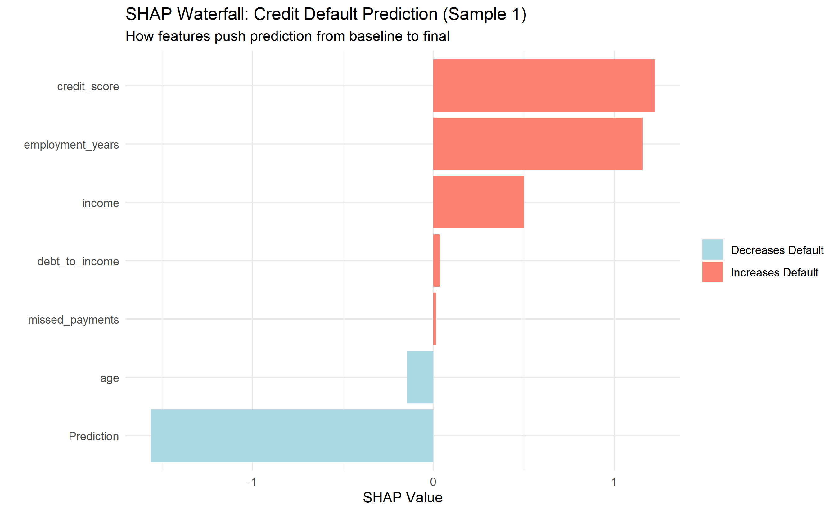
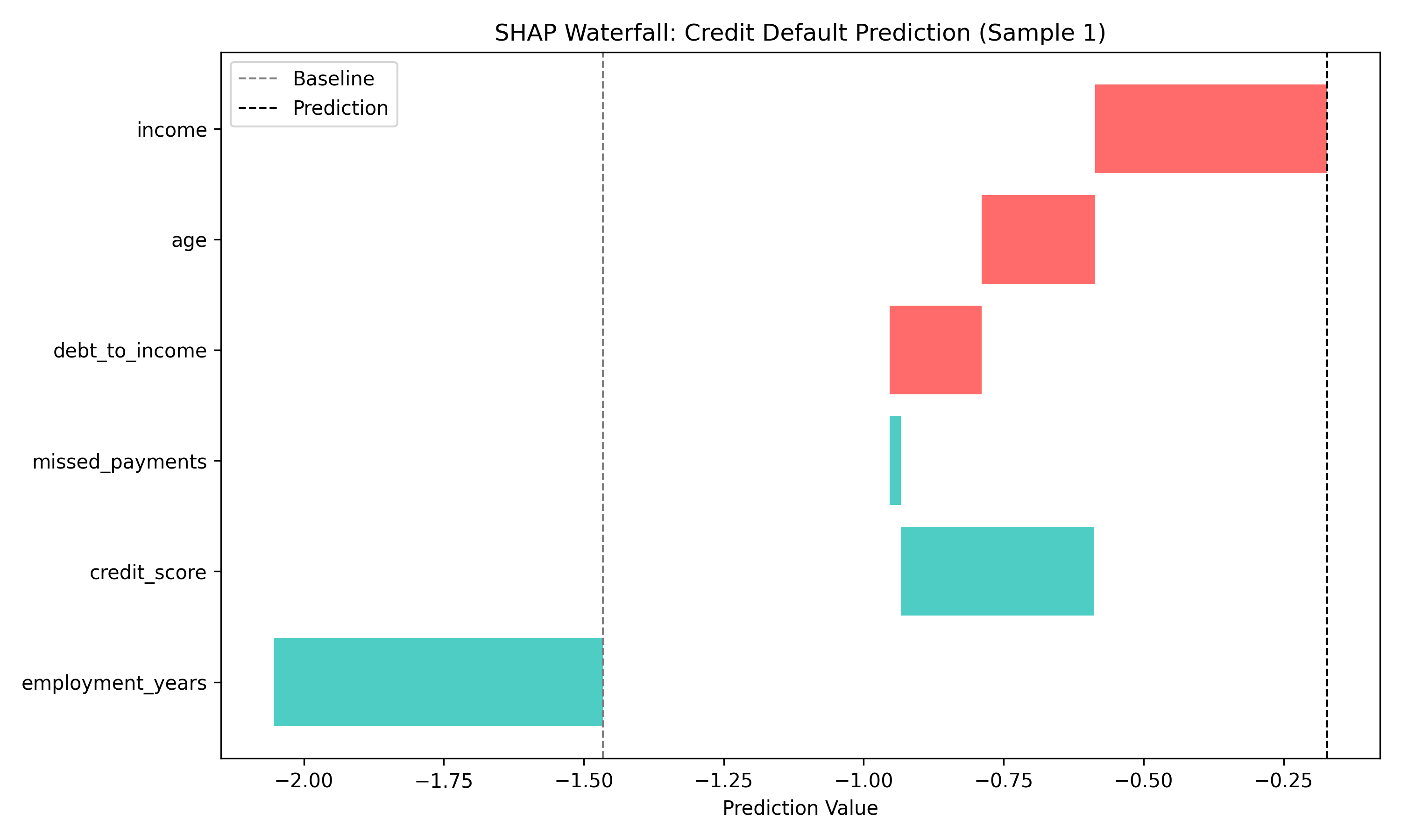
Shows how SHAP values push the prediction from baseline to the final value for a single sample. Useful for explaining individual decisions.
**Beeswarm plot (global + local):**
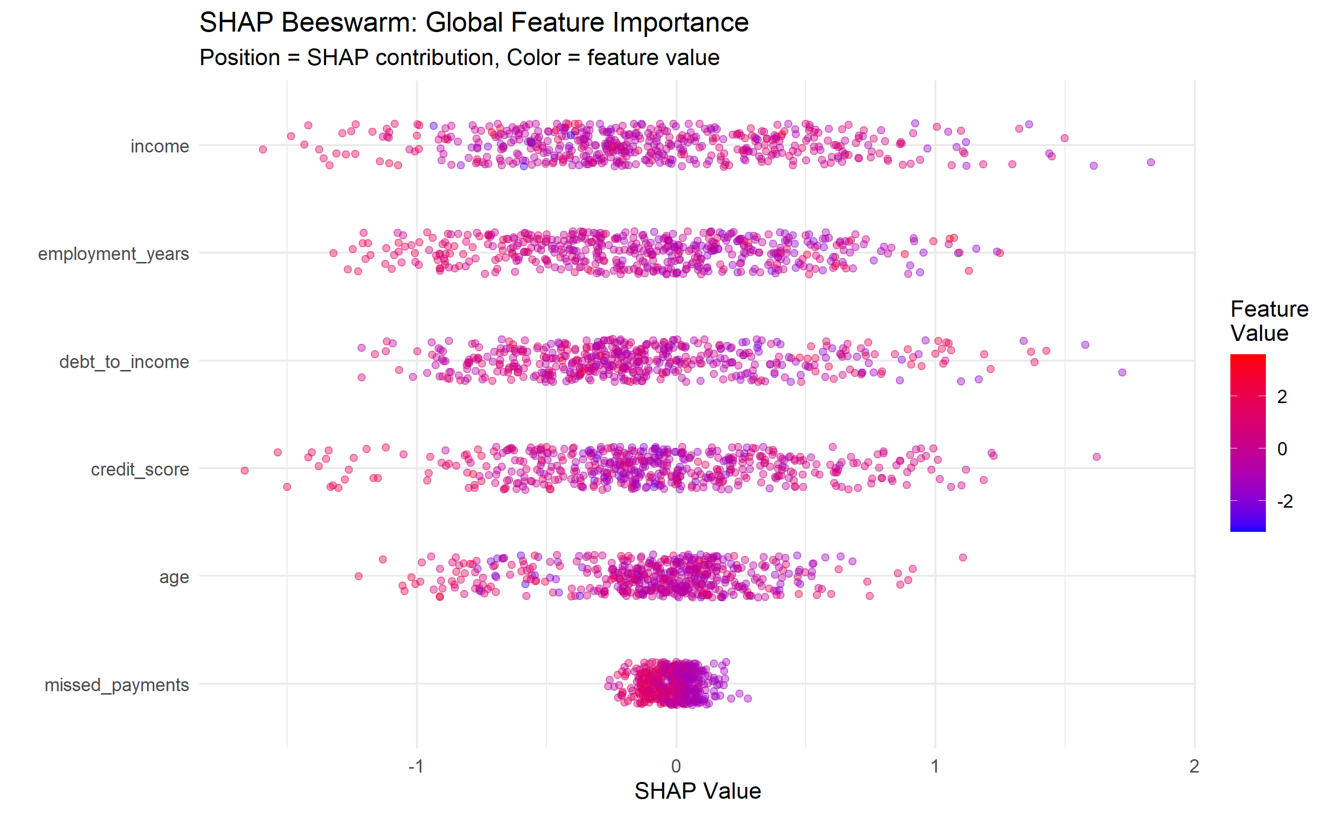
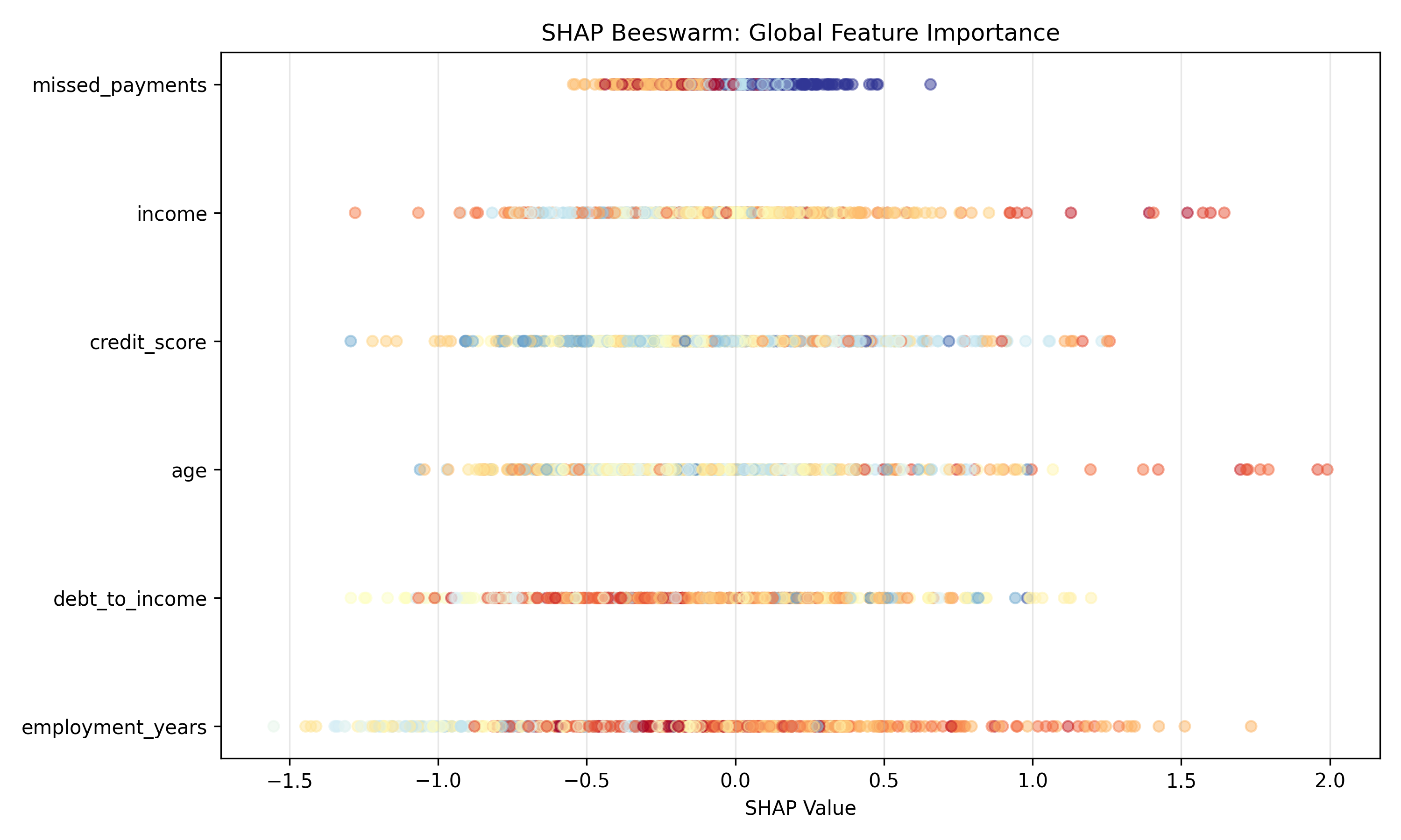
Aggregates SHAP values across all samples. Each dot is a sample, positioned by SHAP value. Color indicates feature value (red = high, blue = low). Reveals global feature importance and direction of effect.
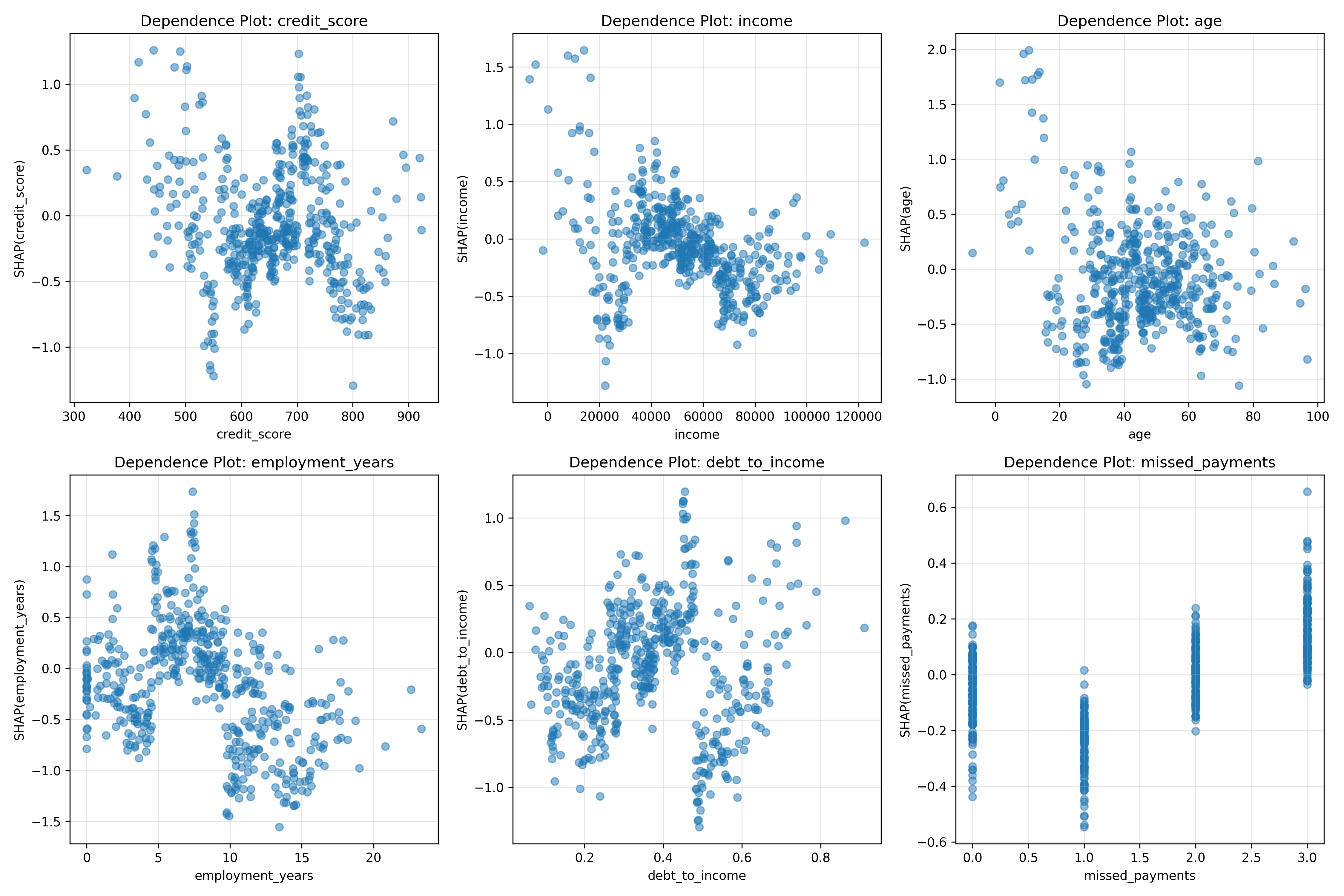
**Dependence plot (interactions):**
Scatter plot of feature value vs. SHAP value. Shows the relationship: does increasing a feature increase its SHAP contribution? Reveals non-linearities and interactions.
**Force plot:**
Alternative visualization of waterfall; shows a stacked bar of feature contributions.
:::
### Creating SHAP Plots
::: {.panel-tabset}
## R
```{r}
# SHAP plots (using shapviz or base R)

# 1. Waterfall plot for sample 1
shap_sample1 <- data.frame(
  Feature = c("Baseline", colnames(X_matrix), "Prediction"),
  Value = c(baseline, shap_contrib, pred)
)

# Cumulative for plotting
shap_sample1$Cumulative <- cumsum(shap_sample1$Value)
shap_sample1$CumulativePrev <- c(0, shap_sample1$Cumulative[-nrow(shap_sample1)])

ggplot(shap_sample1[-1, ], aes(x = reorder(Feature, Value), y = Value)) +
  geom_col(aes(fill = Value > 0)) +
  coord_flip() +
  labs(title = "SHAP Waterfall: Credit Default Prediction (Sample 1)",
       subtitle = "How features push prediction from baseline to final",
       x = "", y = "SHAP Value") +
  theme_minimal() +
  scale_fill_manual(values = c("TRUE" = "salmon", "FALSE" = "lightblue"),
                   labels = c("TRUE" = "Increases Default", "FALSE" = "Decreases Default")) +
  theme(legend.title = element_blank())
# 2. Beeswarm-style plot (feature importance across all samples)
shap_melted <- as.data.frame(shap_values[, 1:6]) |>
  rownames_to_column("sample") |>
  pivot_longer(cols = -sample, names_to = "Feature", values_to = "SHAP")

# Add feature values for coloring
feature_values <- data.frame()
for (j in 1:6) {
  feature_values <- rbind(feature_values,
    data.frame(sample = as.character(1:nrow(credit_data)),
               Feature = colnames(X_matrix)[j],
               FeatureValue = scale(X_matrix[, j])))
}

shap_melted <- shap_melted |>
  left_join(feature_values, by = c("sample", "Feature"))

ggplot(shap_melted, aes(x = reorder(Feature, SHAP, FUN = function(x) mean(abs(x))),
                        y = SHAP, color = FeatureValue)) +
  geom_jitter(alpha = 0.4, width = 0.2) +
  coord_flip() +
  scale_color_gradient(low = "blue", high = "red", name = "Feature\nValue") +
  labs(title = "SHAP Beeswarm: Global Feature Importance",
       subtitle = "Position = SHAP contribution, Color = feature value",
       x = "", y = "SHAP Value") +
  theme_minimal()
```
## Python
```{python}
import matplotlib.pyplot as plt

# 1. Waterfall plot for sample 1
fig, ax = plt.subplots(figsize=(10, 6))

sample_idx = 0
shap_vals = shap_values_default[sample_idx]
base_value = explainer.expected_value

# Prepare data
plot_data = pd.DataFrame({
    'Feature': X.columns.tolist(),
    'SHAP': shap_vals,
    'Value': X.iloc[sample_idx].values
})
plot_data = plot_data.sort_values('SHAP', ascending=True)

# Cumulative for waterfall
cumsum = plot_data['SHAP'].cumsum()
plot_data['Start'] = cumsum.shift(fill_value=base_value)
plot_data['End'] = cumsum

# Plot
colors = ['#FF6B6B' if x > 0 else '#4ECDC4' for x in plot_data['SHAP']]
ax.barh(plot_data['Feature'], plot_data['SHAP'], left=plot_data['Start'], color=colors)
ax.axvline(base_value, color='gray', linestyle='--', linewidth=1, label='Baseline')
ax.axvline(plot_data['End'].iloc[-1], color='black', linestyle='--', linewidth=1, label='Prediction')
ax.set_xlabel('Prediction Value')
ax.set_title('SHAP Waterfall: Credit Default Prediction (Sample 1)')
ax.legend()
plt.tight_layout()
plt.savefig('shap_waterfall.png', dpi=100, bbox_inches='tight')
plt.show()
# 2. Beeswarm plot
fig, ax = plt.subplots(figsize=(10, 6))

# Compute mean absolute SHAP for ordering
mean_abs_shap = np.abs(shap_values_default).mean(axis=0)
feature_order = np.argsort(mean_abs_shap)[::-1]

for idx, feature_idx in enumerate(feature_order):
    values = shap_values_default[:, feature_idx]
    features_vals = X.iloc[:, feature_idx].values

    # Normalize feature values for coloring
    norm_vals = (features_vals - features_vals.min()) / (features_vals.max() - features_vals.min())

    ax.scatter(values, [idx] * len(values), c=norm_vals, cmap='RdYlBu', alpha=0.5, s=30)

ax.set_yticks(range(len(feature_order)))
ax.set_yticklabels([X.columns[i] for i in feature_order])
ax.set_xlabel('SHAP Value')
ax.set_title('SHAP Beeswarm: Global Feature Importance')
ax.grid(axis='x', alpha=0.3)
plt.tight_layout()
plt.savefig('shap_beeswarm.png', dpi=100, bbox_inches='tight')
plt.show()
# 3. Dependence plot (feature interaction)
fig, axes = plt.subplots(2, 3, figsize=(15, 10))
axes = axes.flatten()

for idx, feature_idx in enumerate(range(6)):
    ax = axes[idx]
    feature_name = X.columns[feature_idx]

    ax.scatter(X.iloc[:, feature_idx], shap_values_default[:, feature_idx], alpha=0.5)
    ax.set_xlabel(feature_name)
    ax.set_ylabel(f'SHAP({feature_name})')
    ax.set_title(f'Dependence Plot: {feature_name}')
    ax.grid(alpha=0.3)

plt.tight_layout()
plt.savefig('shap_dependence.png', dpi=100, bbox_inches='tight')
plt.show()
```
:::
::: {.callout-caution icon="false"}
## 📝 Section 16.4 Review Questions
1. In a waterfall plot, why do features appear in a specific order?
2. In a beeswarm plot, what does a vertical spread of dots indicate?
3. In a dependence plot, what would a non-linear relationship suggest about the model?
4. For a categorical feature (e.g., employment sector), how would you create SHAP plots?
:::
## LIME: Local Interpretable Model-Agnostic Explanations
While SHAP is grounded in game theory, **LIME** takes a simpler, more direct approach: fit an **interpretable surrogate model** locally around a prediction.
::: {.callout-note icon="false"}
## 📘 Theory: LIME Algorithm
**Key idea:**
To explain a complex model's prediction for sample x, we:
1. Perturb x slightly to create a local neighborhood.
2. Get model predictions on perturbed samples.
3. Fit a simple, interpretable model (e.g., logistic regression) to the perturbed data, weighted by distance to x.
4. The simple model's coefficients are the LIME explanation.
**Algorithm:**
```
for i = 1 to N_perturbations:
    x_perturbed ← perturb features of original sample x
    distance_i ← distance(x, x_perturbed)
    weight_i ← kernel(distance_i)  // exponential or other kernel
    y_pred_i ← complex_model(x_perturbed)

surrogate_model ← fit interpretable_model(x_perturbed, y_pred_i, weights)
explanation ← coefficients of surrogate_model
```
**Advantages:**
- Model-agnostic: works for any model (neural networks, black boxes, etc.).
- Intuitive: the surrogate model is directly interpretable.
- Fast: doesn't require Shapley value computation.
**Disadvantages:**
- Not theoretically grounded (no axioms like SHAP).
- Sensitive to perturbation method and choice of surrogate model.
- Local explanation only (no global view).
:::
### LIME for Credit Default Prediction
::: {.panel-tabset}
## R
```{r}
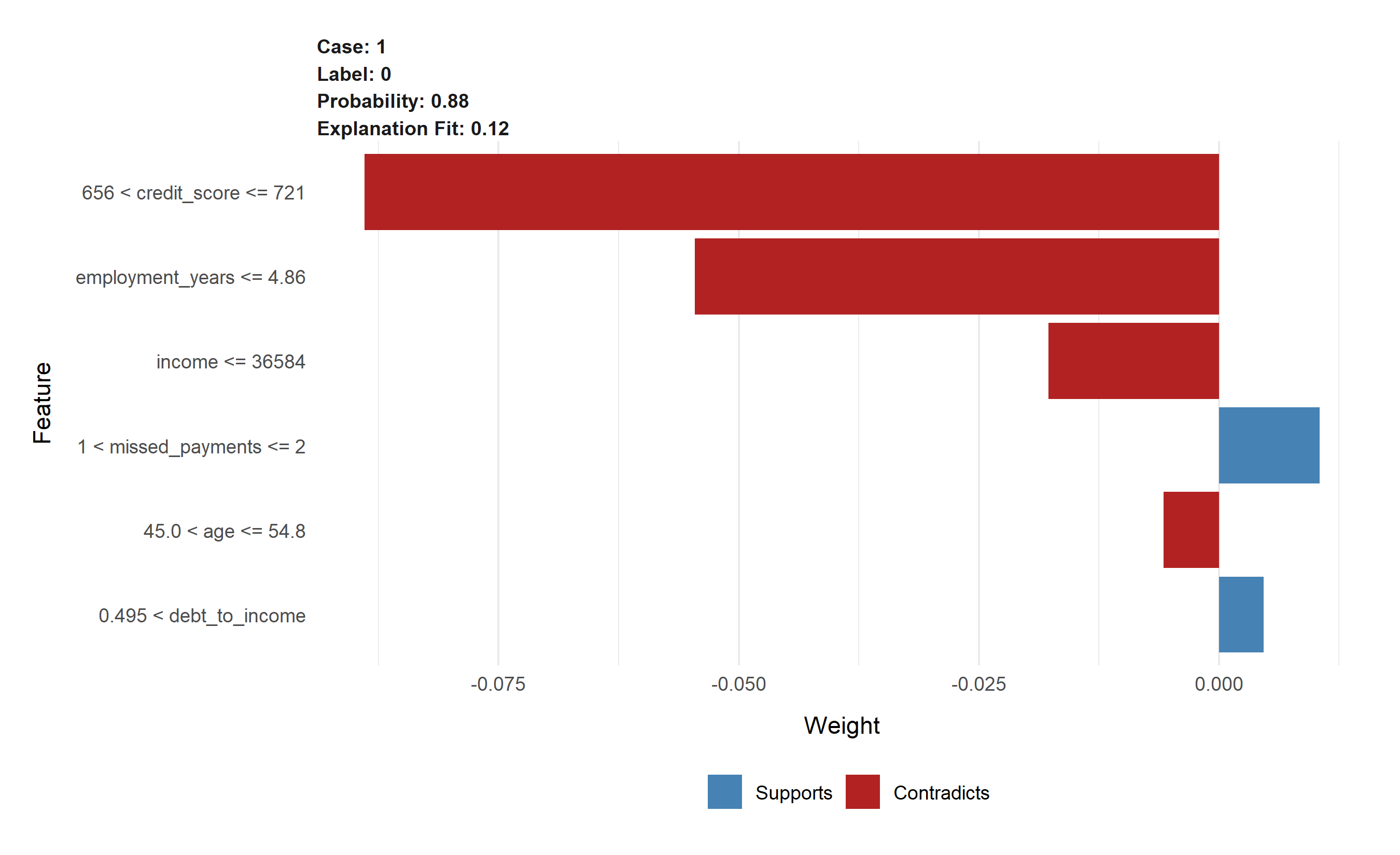
library(lime)
# LIME explanation
# Create LIME explainer
lime_explainer <- lime(credit_data[, 1:6], xgb_model,
bin_continuous = TRUE)
# Explain a few samples
sample_indices <- c(1, 50, 100)
for (idx in sample_indices) {
cat("\n=== LIME Explanation for Sample", idx, "===\n")
explanation <- explain(credit_data[idx, 1:6],
explainer = lime_explainer,
n_features = 6,
n_labels = 1,
kernel_width = 0.25)
print(explanation)
}
# Visualize
plot_features(explanation)
```
## Python
```{python}
from lime.lime_tabular import LimeTabularExplainer
# Create LIME explainer
lime_explainer = LimeTabularExplainer(
X.values,
feature_names=X.columns.tolist(),
class_names=['No Default', 'Default'],
mode='classification',
random_state=2026
)
# Explain sample 0
sample_idx = 0
explanation = lime_explainer.explain_instance(
X.iloc[sample_idx].values,
xgb_model.predict_proba,
num_features=6,
top_labels=2
)
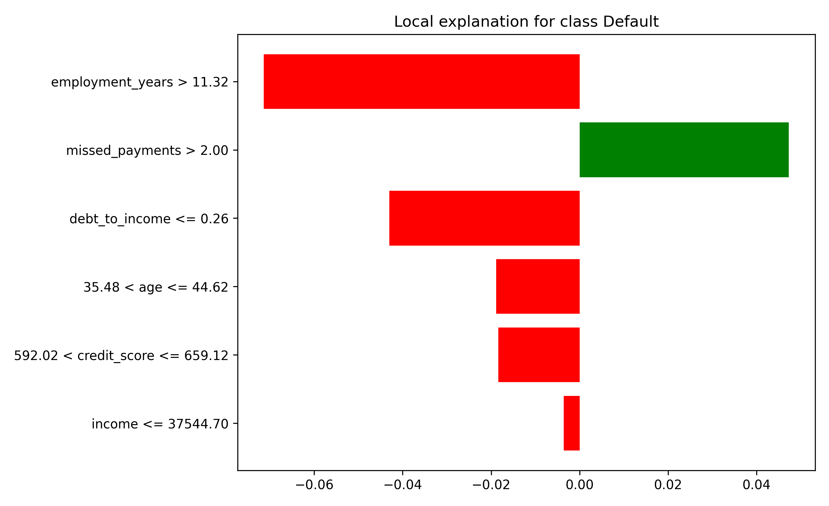
print("=== LIME Explanation for Sample 0 ===")
print(f"Prediction: {xgb_model.predict_proba(X.iloc[[sample_idx]])[0]}")
print(f"\nInterpretable Model (surrogate) coefficients:")
for feature, weight in explanation.as_list(label=1): # class 1 = default
print(f" {feature}: {weight:+.4f}")
# Visualize
fig = explanation.as_pyplot_figure(label=1)
plt.tight_layout()
plt.savefig('lime_explanation.png', dpi=100, bbox_inches='tight')
plt.show()
# Explain multiple samples
print("\n\n=== LIME Explanations for Multiple Samples ===\n")
for idx in [0, 50, 100]:
explanation = lime_explainer.explain_instance(
X.iloc[idx].values,
xgb_model.predict_proba,
num_features=4
)
print(f"Sample {idx}:")
for feature, weight in explanation.as_list(label=1):
print(f" {feature}: {weight:+.4f}")
print()
```
:::
::: {.callout-caution icon="false"}
## 📝 Section 16.5 Review Questions
1. Why is LIME called "model-agnostic" while SHAP is not?
2. How does LIME's surrogate model differ from SHAP's game-theoretic approach?
3. What is the role of the "kernel" in LIME? How does it weight perturbed samples?
4. When would you prefer LIME over SHAP, and vice versa?
:::
## Model Cards and Responsible AI
A **model card** documents a model's performance, limitations, and fairness metrics. It bridges the gap between technical teams and business stakeholders.
::: {.callout-note icon="false"}
## 📘 Theory: Model Cards and Fairness Metrics
**Model card components:**
1. **Model details:** Name, version, authors, date, intended use.
2. **Performance metrics:** AUC, F1, accuracy across overall dataset.
3. **Performance by group:** Breakdown by demographic groups (age, gender, location).
4. **Fairness metrics:**
- **Demographic parity:** P(Ŷ=1 | A=0) = P(Ŷ=1 | A=1) for protected attribute A.
- **Equalized odds:** False Positive Rate and True Positive Rate equal across groups.
- **Calibration:** Predicted probabilities match actual rates within each group.
5. **Limitations:** Known failure modes, biases, out-of-distribution scenarios.
6. **Training data:** Description, representativeness, data provenance.
**Why model cards matter:**
- Transparency: stakeholders understand what the model does and doesn't do.
- Accountability: documented fairness assessment reduces legal risk.
- Maintainability: clear limitations guide retraining decisions.
:::
### Building a Model Card for Credit Default
::: {.panel-tabset}
## R
```{r}
library(tidyverse)
# Simulate demographic groups
credit_data_with_groups <- credit_data |>
mutate(
age_group = case_when(age < 35 ~ "Young (< 35)",
age < 50 ~ "Middle (35-50)",
TRUE ~ "Senior (> 50)"),
gender = sample(c("M", "F"), n(), replace = TRUE),
region = sample(c("North", "South", "East", "West"), n(), replace = TRUE)
)
# Overall performance
overall_pred <- as.numeric(predict(xgb_model, dtrain, type = "class")) - 1
overall_auc <- as.numeric(auc(y_vector, overall_pred))
cat("=== MODEL CARD: CREDIT DEFAULT PREDICTION ===\n\n")
cat("## Model Details\n")
cat("Name: Credit Default XGBoost Classifier\n")
cat("Version: 1.0\n")
cat("Date: 2026-04-11\n")
cat("Authors: Bongo Adi\n")
cat("Framework: XGBoost\n")
cat("Intended Use: Evaluate credit default risk for new applicants\n\n")
cat("## Overall Performance\n")
cat(sprintf("AUC: %.4f\n", overall_auc))
cat(sprintf("Accuracy: %.4f\n", mean(overall_pred == y_vector)))
cat("\n")
# Performance by age group
cat("## Performance by Age Group\n")
age_group_perf <- credit_data_with_groups |>
mutate(pred = overall_pred) |>
group_by(age_group) |>
summarise(
n = n(),
auc = as.numeric(auc(default, pred)),
pred_default_rate = mean(pred),
actual_default_rate = mean(default),
.groups = 'drop'
)
print(age_group_perf)
# Demographic parity check
cat("\n## Fairness Analysis: Demographic Parity\n")
demo_parity <- credit_data_with_groups |>
mutate(pred = overall_pred) |>
group_by(gender) |>
summarise(
default_prediction_rate = mean(pred),
.groups = 'drop'
)
cat("Predicted default rate by gender:\n")
print(demo_parity)
parity_diff <- abs(demo_parity$default_prediction_rate[1] -
demo_parity$default_prediction_rate[2])
cat(sprintf("\nDifference: %.4f (fairness threshold: < 0.05)\n", parity_diff))
# Calibration by group
cat("\n## Calibration by Region\n")
calibration <- credit_data_with_groups |>
mutate(
pred_prob = overall_pred,
pred_bucket = cut(pred_prob, breaks = seq(0, 1, 0.2), include.lowest = TRUE)
) |>
group_by(region, pred_bucket) |>
summarise(
actual_rate = mean(default),
n = n(),
.groups = 'drop'
) |>
filter(!is.na(pred_bucket))
print(calibration)
cat("\n## Known Limitations\n")
cat("1. Model trained on 2026 data; may not reflect 2027 loan patterns\n")
cat("2. Limited geographic diversity (synthetic data)\n")
cat("3. No recency weighting; old defaults treated same as recent\n")
cat("4. Income is self-reported; high measurement error\n")
```
## Python
```{python}
# Add demographic groups
credit_data_with_groups = credit_data.copy()
credit_data_with_groups['age_group'] = pd.cut(
credit_data_with_groups['age'],
bins=[0, 35, 50, 100],
labels=['Young (< 35)', 'Middle (35-50)', 'Senior (> 50)']
)
credit_data_with_groups['gender'] = np.random.choice(['M', 'F'], len(credit_data))
credit_data_with_groups['region'] = np.random.choice(
['North', 'South', 'East', 'West'], len(credit_data)
)
# Overall performance
y_pred = xgb_model.predict(X)
y_pred_proba = xgb_model.predict_proba(X)[:, 1]
from sklearn.metrics import auc, roc_auc_score, accuracy_score
overall_auc = roc_auc_score(y, y_pred_proba)
overall_acc = accuracy_score(y, y_pred)
print("=" * 50)
print("MODEL CARD: CREDIT DEFAULT PREDICTION")
print("=" * 50)
print()
print("## Model Details")
print("Name: Credit Default XGBoost Classifier")
print("Version: 1.0")
print("Date: 2026-04-11")
print("Authors: Bongo Adi")
print("Framework: XGBoost")
print("Intended Use: Evaluate credit default risk for new applicants\n")
print("## Overall Performance")
print(f"AUC: {overall_auc:.4f}")
print(f"Accuracy: {overall_acc:.4f}\n")
# Performance by age group
print("## Performance by Age Group")
age_group_perf = credit_data_with_groups.groupby('age_group').apply(
lambda group: pd.Series({
'n': len(group),
'auc': roc_auc_score(group['default'], y_pred_proba[group.index]),
'pred_default_rate': y_pred[group.index].mean(),
'actual_default_rate': group['default'].mean()
})
)
print(age_group_perf)
print()
# Demographic parity
print("## Fairness Analysis: Demographic Parity")
demo_parity = credit_data_with_groups.groupby('gender').apply(
lambda group: y_pred[group.index].mean()
)
print("Predicted default rate by gender:")
print(demo_parity)
parity_diff = abs(demo_parity.iloc[0] - demo_parity.iloc[1])
print(f"\nDifference: {parity_diff:.4f} (fairness threshold: < 0.05)")
# Calibration
print("\n## Calibration by Region")
credit_data_with_groups['pred_prob'] = y_pred_proba
credit_data_with_groups['pred_bucket'] = pd.cut(
credit_data_with_groups['pred_prob'],
bins=[0, 0.2, 0.4, 0.6, 0.8, 1.0]
)
calibration = credit_data_with_groups.groupby(['region', 'pred_bucket']).apply(
lambda group: pd.Series({
'actual_rate': group['default'].mean(),
'n': len(group)
})
)
print(calibration)
print("\n## Known Limitations")
print("1. Model trained on 2026 data; may not reflect 2027 loan patterns")
print("2. Limited geographic diversity (synthetic data)")
print("3. No recency weighting; old defaults treated same as recent")
print("4. Income is self-reported; high measurement error")
```
:::
::: {.callout-caution icon="false"}
## 📝 Section 16.6 Review Questions
1. What is the difference between demographic parity and equalized odds?
2. If demographic parity is violated, what action would you take?
3. How would you measure whether a model is "calibrated"?
4. Why should model cards be updated regularly?
:::
## Case Study: Explaining a Credit Decision to a Loan Officer
In this case study, we demonstrate the full workflow: fit a model, explain it locally using SHAP, and role-play presenting it to a loan officer.
::: {.panel-tabset}
## R
```{r}
# Scenario: Three loan applicants with contrasting SHAP profiles
cat("=== LOAN DECISION EXPLANATION MEETING ===\n\n")
# Create three representative applicants
applicants <- data.frame(
applicant_id = c("A001", "A002", "A003"),
credit_score = c(750, 600, 680),
income = c(80000, 35000, 55000),
age = c(50, 28, 45),
employment_years = c(15, 2, 8),
debt_to_income = c(0.2, 0.6, 0.35),
missed_payments = c(0, 2, 0)
)
cat("Applicants for review:\n")
print(applicants)
# Prepare for prediction
X_applicants <- as.matrix(applicants[, -1])
predictions <- predict(xgb_model, xgb.DMatrix(X_applicants))
# Get SHAP values
dtrain_applicants <- xgb.DMatrix(X_applicants)
shap_applicants <- predict(xgb_model, dtrain_applicants, predcontrib = TRUE)
cat("\n## Applicant A001: APPROVED (Low Default Risk)\n\n")
cat("Prediction probability:", round(predictions[1], 4), "\n")
cat("Recommendation: APPROVE - Low risk profile\n\n")
cat("SHAP Explanation:\n")
baseline_pred <- shap_applicants[1, 7]
for (j in 1:6) {
feature_val <- applicants[1, j+1]
shap_val <- shap_applicants[1, j]
feature_name <- colnames(X_applicants)[j]
direction <- ifelse(shap_val > 0, "INCREASES default risk", "DECREASES default risk")
cat(sprintf("%s (%.2f): %+.4f (%s)\n", feature_name, feature_val, shap_val, direction))
}
cat("\nKey strengths:\n")
cat("- High credit score (750): indicates responsible payment history\n")
cat("- High income (₦80,000): sufficient to repay\n")
cat("- No missed payments: clean payment record\n\n")
cat("---\n\n")
cat("## Applicant A002: REVIEW REQUIRED (High Default Risk)\n\n")
cat("Prediction probability:", round(predictions[2], 4), "\n")
cat("Recommendation: REFER TO REVIEW - High risk profile, consider additional verification\n\n")
cat("SHAP Explanation:\n")
for (j in 1:6) {
feature_val <- applicants[2, j+1]
shap_val <- shap_applicants[2, j]
feature_name <- colnames(X_applicants)[j]
direction <- ifelse(shap_val > 0, "INCREASES default risk", "DECREASES default risk")
cat(sprintf("%s (%.2f): %+.4f (%s)\n", feature_name, feature_val, shap_val, direction))
}
cat("\nKey concerns:\n")
cat("- Low credit score (600): indicator of past payment issues\n")
cat("- High debt-to-income (0.60): limited income after obligations\n")
cat("- Recent missed payments (2): shows current difficulty\n")
cat("- Short employment (2 years): unstable income history\n\n")
cat("---\n\n")
cat("## Applicant A003: CONDITIONAL APPROVAL (Moderate Risk)\n\n")
cat("Prediction probability:", round(predictions[3], 4), "\n")
cat("Recommendation: APPROVE WITH CONDITIONS - Request collateral or co-signer\n\n")
cat("SHAP Explanation:\n")
for (j in 1:6) {
feature_val <- applicants[3, j+1]
shap_val <- shap_applicants[3, j]
feature_name <- colnames(X_applicants)[j]
direction <- ifelse(shap_val > 0, "INCREASES default risk", "DECREASES default risk")
cat(sprintf("%s (%.2f): %+.4f (%s)\n", feature_name, feature_val, shap_val, direction))
}
cat("\nProfile summary:\n")
cat("- Mixed signals: reasonable income and clean payment history\n")
cat("- Moderate debt load and moderate credit score\n")
cat("- Recommendation: approve with 5% higher interest rate to offset risk\n")
```
## Python
```{python}
# Three representative applicants
applicants_data = pd.DataFrame({
'credit_score': [750, 600, 680],
'income': [80000, 35000, 55000],
'age': [50, 28, 45],
'employment_years': [15, 2, 8],
'debt_to_income': [0.2, 0.6, 0.35],
'missed_payments': [0, 2, 0]
}, index=['A001', 'A002', 'A003'])
print("=" * 60)
print("LOAN DECISION EXPLANATION MEETING")
print("=" * 60)
print()
print("Applicants for review:")
print(applicants_data)
print()
# Predictions
applicant_pred = xgb_model.predict_proba(applicants_data)[:, 1]
applicant_shap = explainer.shap_values(applicants_data)
if isinstance(applicant_shap, list):
applicant_shap = applicant_shap[1]
base_value = explainer.expected_value
for idx, applicant_id in enumerate(['A001', 'A002', 'A003']):
print()
print("=" * 60)
if idx == 0:
print(f"## Applicant {applicant_id}: APPROVED (Low Default Risk)")
recommendation = "APPROVE"
elif idx == 1:
print(f"## Applicant {applicant_id}: REVIEW REQUIRED (High Default Risk)")
recommendation = "REFER TO REVIEW"
else:
print(f"## Applicant {applicant_id}: CONDITIONAL APPROVAL (Moderate Risk)")
recommendation = "APPROVE WITH CONDITIONS"
print()
print(f"Prediction probability: {applicant_pred[idx]:.4f}")
print(f"Recommendation: {recommendation}")
print()
print("SHAP Explanation (Feature Contributions):")
for j, feature_name in enumerate(X.columns):
feature_val = applicants_data.iloc[idx, j]
shap_val = applicant_shap[idx, j]
direction = "INCREASES default risk" if shap_val > 0 else "DECREASES default risk"
print(f" {feature_name} ({feature_val:.2f}): {shap_val:+.4f} ({direction})")
# Commentary
if idx == 0:
print("\nKey strengths:")
print(" - High credit score (750): indicates responsible payment history")
print(" - High income (₦80,000): sufficient to repay")
print(" - No missed payments: clean payment record")
elif idx == 1:
print("\nKey concerns:")
print(" - Low credit score (600): indicator of past payment issues")
print(" - High debt-to-income (0.60): limited income after obligations")
print(" - Recent missed payments (2): shows current difficulty")
print(" - Short employment (2 years): unstable income history")
else:
print("\nProfile summary:")
print(" - Mixed signals: reasonable income and clean payment history")
print(" - Moderate debt load and moderate credit score")
print(" - Recommendation: approve with 5% higher interest rate to offset risk")
print()
print("=" * 60)
```
:::
::: {.callout-caution icon="false"}
## 📝 Section 16.7 Review Questions
1. Why is it important to explain individual decisions (not just global importance)?
2. If an applicant questions a rejection decision, how would you use SHAP to justify it?
3. In the case study, which applicant is most "borderline"? How would you handle this case?
4. What risks arise if loan officers override model decisions without understanding explanations?
:::
## Chapter 16 Exercises
::: {.exercises}
1. **SHAP vs. LIME:** Train both on the same credit default model. Compare the explanations for the same sample. Which is clearer to a business stakeholder?
2. **Global explanation:** Create a SHAP summary plot showing which features matter most across all predictions.
3. **Fairness audit:** Build a model card for your predictive model. Check demographic parity across age and gender groups.
4. **Waterfall plot:** Create SHAP waterfall explanations for two contrasting applicants (one approved, one rejected).
5. **Interaction detection:** Use SHAP dependence plots to identify feature interactions in your model.
6. **LIME sensitivity:** Train LIME with different kernel widths. How does the explanation change?
7. **Counterfactual explanation:** For a rejected applicant, compute the minimal feature changes needed for approval.
8. **Model improvement:** Use explainability to identify if the model relies on a problematic feature (e.g., zip code as proxy for race).
9. **Stakeholder communication:** Draft a 1-page explanation of a model decision suitable for a non-technical loan officer.
10. **Regulatory compliance:** Document fairness metrics for an equal employment opportunity audit.
:::
## Further Reading
1. **Lundberg, S. M., & Lee, S.-I.** (2017). "A unified approach to interpreting model predictions." *NIPS*, 4768–4777. — Original SHAP paper.
2. **Ribeiro, M. T., Singh, S., & Guestrin, C.** (2016). ""Why should I trust you?": Explaining the predictions of any classifier." *KDD*, 1135–1144. — Original LIME paper.
3. **Molnar, C.** (2020). *Interpretable Machine Learning: A Guide for Making Black-Box Models Explainable.* [https://christophmolnar.com/books/interpretable-ml/] — Comprehensive guide to explainability techniques.
4. **Arrieta, A. B., Díaz-Rodríguez, N., et al.** (2020). "Explainable artificial intelligence (XAI): concepts, taxonomies, opportunities and challenges toward responsible AI." *Information Fusion*, 58, 82–115. — Survey of XAI methods.
5. **Mitchell, M., Wu, S., et al.** (2019). "Model cards for model reporting." *FAccT*, 220–229. — Framework for model cards and documentation.
## Chapter 16 Appendix
### A. Derivation of Shapley Values
**Theorem (Shapley, 1953):** The unique value function satisfying efficiency, symmetry, dummy, and additivity axioms is:
$$\phi_i = \frac{1}{|N|!} \sum_{S \subseteq N \setminus \{i\}} |S|! (|N| - |S| - 1)! [v(S \cup \{i\}) - v(S)]$$
where:
- N is the set of all players (features).
- S is a coalition not containing player i.
- v(S) is the payoff (value) of coalition S.
**For SHAP:**
- Players = features.
- v(S) = expected model prediction when features in S are known (marginalized over background data).
- Payoff = contribution to moving from baseline to prediction.
**Computational complexity:**
Computing exact Shapley values requires summing over 2^p coalitions, which is prohibitive for large p. This is why approximations (Kernel SHAP, TreeSHAP) are necessary.
### B. LIME Kernel and Perturbation
**Exponential kernel for distance weighting:**
$$w_i = \exp\left( -\frac{d_i^2}{\sigma^2} \right)$$
where:
- $d_i$ is the distance between original sample x and perturbed sample $x_i$.
- σ is the kernel width (controls locality).
A small σ means only very close neighbors are weighted; large σ means distant neighbors matter too. This is a key hyperparameter in LIME.
**Perturbation strategies:**
For continuous features:
- Sample from a normal distribution: $x_j^{pert} \sim N(x_j, 0.2 \sigma_{training})$
For categorical features:
- Randomly select a value: $x_j^{pert} \in \{Category_1, \ldots, Category_k\}$ with equal probability.
The choice of perturbation significantly affects LIME explanations.
### C. Fairness Metrics Definitions
**Demographic Parity:**
$$P(\hat{Y}=1 | A=0) = P(\hat{Y}=1 | A=1)$$
The positive prediction rate should be equal across protected groups A.
**Equalized Odds:**
$$P(\hat{Y}=1 | A=0, Y=1) = P(\hat{Y}=1 | A=1, Y=1)$$ and $$P(\hat{Y}=1 | A=0, Y=0) = P(\hat{Y}=1 | A=1, Y=0)$$
True positive and false positive rates should be equal across groups.
**Calibration:**
$$P(Y=1 | \hat{Y}=p, A=0) = P(Y=1 | \hat{Y}=p, A=1) \approx p$$
For samples predicted to have probability p of positive class, the actual positive rate should equal p, within each group.
---
*End of Chapter 16*