---
title: "Introduction to Unsupervised Learning"
author: "Bongo Adi"
date: "2024"
number-sections: true
---
```{python}
#| label: python-setup-19-intro-unsupervised
#| include: false
import os
import numpy as np
import pandas as pd
import matplotlib.pyplot as plt
import seaborn as sns
from scipy.spatial.distance import pdist, squareform, cdist, mahalanobis
from scipy.stats import gaussian_kde
from sklearn.cluster import KMeans
from sklearn.preprocessing import StandardScaler, RobustScaler
from sklearn.metrics import (silhouette_score, pairwise_distances,
calinski_harabasz_score, davies_bouldin_score)
os.environ['OMP_NUM_THREADS'] = '1'
```
::: {.callout-note icon="false"}
## 📋 Learning Objectives
By the end of this chapter, you will:
- Distinguish supervised from unsupervised learning and understand when labels are unavailable or impractical to obtain
- Recognize four major classes of unsupervised tasks: clustering, dimensionality reduction, density estimation, and anomaly detection
- Compute and interpret four distance metrics (Euclidean, Manhattan, Cosine, Mahalanobis) on real business data
- Understand why feature scaling is critical for distance-based algorithms and implement three scaling strategies
- Evaluate clustering quality without ground truth labels using internal and external validation metrics
- Introduce a realistic mobile money dataset that will anchor Chapters 20 and 21
:::
## Supervised vs. Unsupervised Learning: The Discovery Mindset
In the previous chapters of this text, we have operated in the supervised learning paradigm. We possessed a target variable—whether a customer churned, whether a loan would default, whether a transaction was fraudulent—and our algorithms learned to predict it. The label was our compass. Every model had clear success metrics: accuracy, recall, AUC, mean squared error. We divided our data into train and test sets and measured generalization. This is the world of prediction: we know what we want to forecast, and we measure our success against it.
Unsupervised learning inverts this story. We have features—measurements of customers, products, transactions, regions, or events—but no target variable. No one has labeled the data. Perhaps we have never tried to segment our customer base before, and we do not yet know what segments exist. Perhaps we have sensor readings from a factory, and we wish to discover hidden patterns that might indicate equipment failure. Perhaps we have a survey with hundreds of questions, and we want to reduce them to a handful of latent dimensions. In these scenarios, we are not predicting; we are *discovering*. The mindset shifts from confirmation to exploration.
This discovery mindset is not merely an academic curiosity. In business, many of the most valuable insights come from data we have not yet asked to predict anything. A financial services firm may not know that its customer base breaks naturally into five distinct segments with wildly different profitability profiles until it applies clustering. A retailer may not realize that 40 per cent of its inventory consists of slow-moving, space-hoarding stock until it uses dimensionality reduction to visualize the product portfolio. An operations team may not spot an emerging equipment fault until density-based algorithms flag anomalous behaviour. Unsupervised learning is the toolkit for the questions you have not yet thought to ask.
### Types of Unsupervised Tasks
Unsupervised learning encompasses four primary families of tasks, each suited to different business problems:
**Clustering** groups observations into distinct sets based on similarity. The goal is to ensure that observations within the same cluster are highly similar to one another and observations in different clusters are dissimilar. We cluster customers by purchase behaviour, regions by socioeconomic profile, or transactions by pattern. Clustering answers the question: "Which entities are most alike?"
**Dimensionality reduction** transforms high-dimensional data into a low-dimensional representation that preserves essential structure. If we have a customer described by 50 features, can we summarise that customer in 5 core dimensions? This not only aids visualisation and interpretation but also reduces noise, speeds computation, and mitigates the curse of dimensionality. Dimensionality reduction answers: "What are the essential building blocks of this data?"
**Density estimation** builds a model of the underlying probability distribution of the data. It asks: where are the regions of high density, and where are the regions sparse? Density estimation is the foundation for anomaly detection (sparse regions contain anomalies) and serves in generative modelling. It answers: "How likely is a new observation, and how does it compare to known patterns?"
**Anomaly detection** (also called outlier detection) identifies observations that are unusual, rare, or markedly different from the bulk of the data. In finance, anomalies are fraud. In manufacturing, anomalies are faults. In network security, anomalies are intrusions. Most observations are normal; anomalies are the exception—and often the observation of greatest business value.
All four task types share a common challenge: *there is no ground truth label to which we can compare our results*. We cannot compute accuracy or AUC. We must therefore invent new evaluation metrics that measure coherence, separation, and interpretability without reference to a held-out test set. Much of this chapter is devoted to this challenge.
### Why Unsupervised Learning Matters in Business
Every business dataset tells a story, but most stories go unread because the business does not yet know what questions to ask. In a supervised setting, the organisation must first decide what it wants to predict—churn, fraud, conversion—and only then can machine learning teams spring into action. But the initial decision is often made by stakeholders who may lack technical sophistication or may frame the problem in ways that miss the true opportunity. Unsupervised learning inverts this: it lets the data speak first.
Consider a mobile money provider in East Africa. The firm has transaction history for millions of customers, but the product team does not know whether customers should be targeted for a savings product, a lending product, or a merchant payments service. Supervised approaches would require the firm to first hypothesise a target (e.g., "who will take out a loan?") and then label data. Unsupervised clustering reveals the customer segments *as they naturally appear in the data*, and only then does the product team ask: "What products make sense for each segment?" The order is reversed, and often more fruitful.
Furthermore, not every business question has a natural supervised formulation. If we want to understand how many unique customer personas exist, or which regions are most similar for supply chain purposes, or which products are cannibalising one another, clustering or dimensionality reduction is the natural tool. Supervised learning is powerful, but it is not a universal hammer.
There is also a practical argument: **you cannot label everything**. A firm with millions of transactions might easily label a few thousand for fraud detection, but labelling segments is conceptually different. You would be labelling *every single observation*, which is expensive and subjective. Unsupervised discovery scales where manual labelling does not.
::: {.callout-caution icon="false"}
## 📝 Section 19.1 Review Questions
1. Explain why supervised and unsupervised learning require different evaluation strategies. Why can you not simply use accuracy to evaluate a clustering algorithm?
2. Give three business examples (not discussed above) where clustering would provide value before a supervised learning model even exists.
3. Describe the four main families of unsupervised learning tasks and give a real-world example of each.
4. Why is the "discovery mindset" important in exploratory analysis? How does it differ from the prediction mindset?
:::
## Distance and Similarity: Choosing Your Metric
The foundation of nearly all unsupervised learning is the notion of *distance* or *similarity*. Two observations that are close together in the feature space are considered similar. Two observations far apart are considered dissimilar. This intuition is so fundamental that much of unsupervised learning consists of: (1) defining what "close" means, and (2) grouping observations based on closeness.
Distance metrics are not interchangeable. The choice of metric can dramatically affect the results of clustering, the construction of neighbourhood graphs, and the computational cost of algorithms. In this section, we develop four widely used metrics and discuss when each is appropriate. We then compute all four on a realistic dataset of Nigerian customer profiles.
### Euclidean Distance
The **Euclidean distance** is the straight-line distance between two points in multi-dimensional space. For two observations $\mathbf{x}$ and $\mathbf{y}$ in $\mathbb{R}^p$, the Euclidean distance is:
$$d_E(\mathbf{x}, \mathbf{y}) = \sqrt{\sum_{j=1}^{p} (x_j - y_j)^2}$$
This is the most familiar distance metric and is deeply embedded in our geometric intuition. It treats all dimensions symmetrically and gives more weight to large differences than to small ones (because of the squaring). Euclidean distance is most appropriate when all variables are continuous, measured in comparable units, and when isotropic behaviour (equal variance in all directions) is reasonable.
The Euclidean distance obeys the metric axioms: non-negativity, symmetry, identity of indiscernibles (distance is zero if and only if the points are identical), and the triangle inequality (the direct path is shorter than any detour). These properties make Euclidean distance well-behaved in most algorithms.
### Manhattan Distance (L1 Distance)
The **Manhattan distance**, also called taxicab or L1 distance, is the sum of absolute differences:
$$d_M(\mathbf{x}, \mathbf{y}) = \sum_{j=1}^{p} |x_j - y_j|$$
Imagine walking on a grid: you cannot cut diagonally, only move horizontally and vertically. The Manhattan distance is the shortest path. It is less sensitive to outliers than Euclidean distance (because we do not square), and it is more interpretable in some domains. If each dimension represents a cost or duration, Manhattan distance gives the total cost or time.
Manhattan distance is often preferred in high-dimensional spaces where the curse of dimensionality makes Euclidean distances nearly equal for most point pairs. It is also the natural metric for integer-valued or ordinal features.
### Cosine Similarity and Distance
The **cosine similarity** measures the angle between two vectors:
$$\text{sim}_C(\mathbf{x}, \mathbf{y}) = \frac{\mathbf{x} \cdot \mathbf{y}}{\|\mathbf{x}\| \cdot \|\mathbf{y}\|}$$
This is a number between -1 and 1 (assuming real-valued vectors, often between 0 and 1 for non-negative data). High cosine similarity means the vectors point in nearly the same direction; low similarity means they point in different directions. The corresponding *cosine distance* is $d_C = 1 - \text{sim}_C$.
Cosine similarity is *scale-invariant*: if you multiply a vector by a constant, cosine similarity does not change. This makes it ideal for text and document analysis (where a document with 10,000 words and one with 5,000 words are comparable in topic), sparse high-dimensional data (e.g., product catalogue matching), and any domain where the *direction* of a vector matters more than its magnitude.
However, cosine similarity does not satisfy the triangle inequality and is not a true metric in the strict mathematical sense. Yet it is still useful and widely applied.
### Mahalanobis Distance
The **Mahalanobis distance** is a generalisation of Euclidean distance that accounts for correlations between variables:
$$d_\text{Maha}(\mathbf{x}, \mathbf{y}) = \sqrt{(\mathbf{x} - \mathbf{y})^T \boldsymbol{\Sigma}^{-1} (\mathbf{x} - \mathbf{y})}$$
where $\boldsymbol{\Sigma}$ is the covariance matrix. If variables are independent and have the same variance, this reduces to Euclidean distance. But if some variables are correlated or have very different variances, Mahalanobis distance adjusts accordingly.
The Mahalanobis distance is powerful but computationally more expensive (requires inverting a $p \times p$ covariance matrix) and requires a larger sample size than Euclidean distance to estimate the covariance matrix reliably. It is particularly useful in anomaly detection and when you have a clear baseline distribution.
### Computing Distances on Nigerian Customer Profiles
We now demonstrate all four metrics on a synthetic dataset of Nigerian mobile money customers. Our dataset comprises 100 customers with four features: total spend in the last 90 days (NGN), transaction frequency (count per month), average transaction value (NGN), and days since last transaction.
::: {.panel-tabset}
## R
```{r}
set.seed(42)
library(tidyverse)
library(proxy)
library(mvtnorm)

# Generate synthetic Nigerian customer data
n_customers <- 100
customers <- tibble(
  customer_id = 1:n_customers,
  total_spend_90d = rnorm(n_customers, mean = 250000, sd = 150000),
  txn_frequency = rpois(n_customers, lambda = 8),
  avg_txn_value = rnorm(n_customers, mean = 32000, sd = 15000),
  days_since_last_txn = rpois(n_customers, lambda = 7)
) |>
  filter(total_spend_90d > 0, avg_txn_value > 0) |>
  slice(1:100)

# Display first few rows
head(customers, 10)
# Standardise features for distance computation
X <- customers |>
select(-customer_id) |>
scale() |>
as.data.frame()
# Select two customers for demonstration
cust_1 <- as.numeric(X[1, ])
cust_2 <- as.numeric(X[2, ])
# Euclidean distance
euclidean_dist <- sqrt(sum((cust_1 - cust_2)^2))
cat("Euclidean distance between customer 1 and 2:", euclidean_dist, "\n")
# Manhattan distance
manhattan_dist <- sum(abs(cust_1 - cust_2))
cat("Manhattan distance between customer 1 and 2:", manhattan_dist, "\n")
# Cosine similarity and distance
cosine_sim <- sum(cust_1 * cust_2) / (sqrt(sum(cust_1^2)) * sqrt(sum(cust_2^2)))
cosine_dist <- 1 - cosine_sim
cat("Cosine similarity between customer 1 and 2:", cosine_sim, "\n")
cat("Cosine distance between customer 1 and 2:", cosine_dist, "\n")
# Mahalanobis distance
# Compute covariance matrix
cov_matrix <- cov(X)
inv_cov <- solve(cov_matrix)
mahal_dist <- sqrt(t(cust_1 - cust_2) %*% inv_cov %*% (cust_1 - cust_2))
cat("Mahalanobis distance between customer 1 and 2:", as.numeric(mahal_dist), "\n")
# Compute pairwise distances for all customers
euclidean_matrix <- as.matrix(dist(X, method = "euclidean"))
manhattan_matrix <- as.matrix(dist(X, method = "manhattan"))
# Cosine distance using proxy package
cosine_matrix <- as.matrix(dist(X, method = "cosine"))
# Mahalanobis for the whole dataset
X_mat <- as.matrix(X) # matrix arithmetic required for %*%
n_rows <- nrow(X_mat)
mahal_matrix <- matrix(0, nrow = n_rows, ncol = n_rows)
for (i in 1:n_rows) {
for (j in i:n_rows) {
diff <- X_mat[i, ] - X_mat[j, ]
d <- sqrt(t(diff) %*% inv_cov %*% diff)
mahal_matrix[i, j] <- d
mahal_matrix[j, i] <- d
}
}
# Summary statistics of distances
cat("\n=== Distance Matrix Summaries ===\n")
cat("Euclidean: min =", round(min(euclidean_matrix[euclidean_matrix > 0]), 3),
", median =", round(median(euclidean_matrix[lower.tri(euclidean_matrix)]), 3),
", max =", round(max(euclidean_matrix), 3), "\n")
cat("Manhattan: min =", round(min(manhattan_matrix[manhattan_matrix > 0]), 3),
", median =", round(median(manhattan_matrix[lower.tri(manhattan_matrix)]), 3),
", max =", round(max(manhattan_matrix), 3), "\n")
cat("Cosine: min =", round(min(cosine_matrix[cosine_matrix > 0]), 3),
", median =", round(median(cosine_matrix[lower.tri(cosine_matrix)]), 3),
", max =", round(max(cosine_matrix), 3), "\n")
cat("Mahalanobis: min =", round(min(mahal_matrix[mahal_matrix > 0]), 3),
", median =", round(median(mahal_matrix[lower.tri(mahal_matrix)]), 3),
", max =", round(max(mahal_matrix), 3), "\n")
# Visualise distance distributions
dist_comparison <- tibble(
Euclidean = euclidean_matrix[lower.tri(euclidean_matrix)],
Manhattan = manhattan_matrix[lower.tri(manhattan_matrix)],
Cosine = cosine_matrix[lower.tri(cosine_matrix)],
Mahalanobis = mahal_matrix[lower.tri(mahal_matrix)]
) |>
pivot_longer(everything(), names_to = "Metric", values_to = "Distance")
ggplot(dist_comparison, aes(x = Distance, fill = Metric)) +
geom_density(alpha = 0.6) +
facet_wrap(~ Metric, scales = "free") +
theme_minimal() +
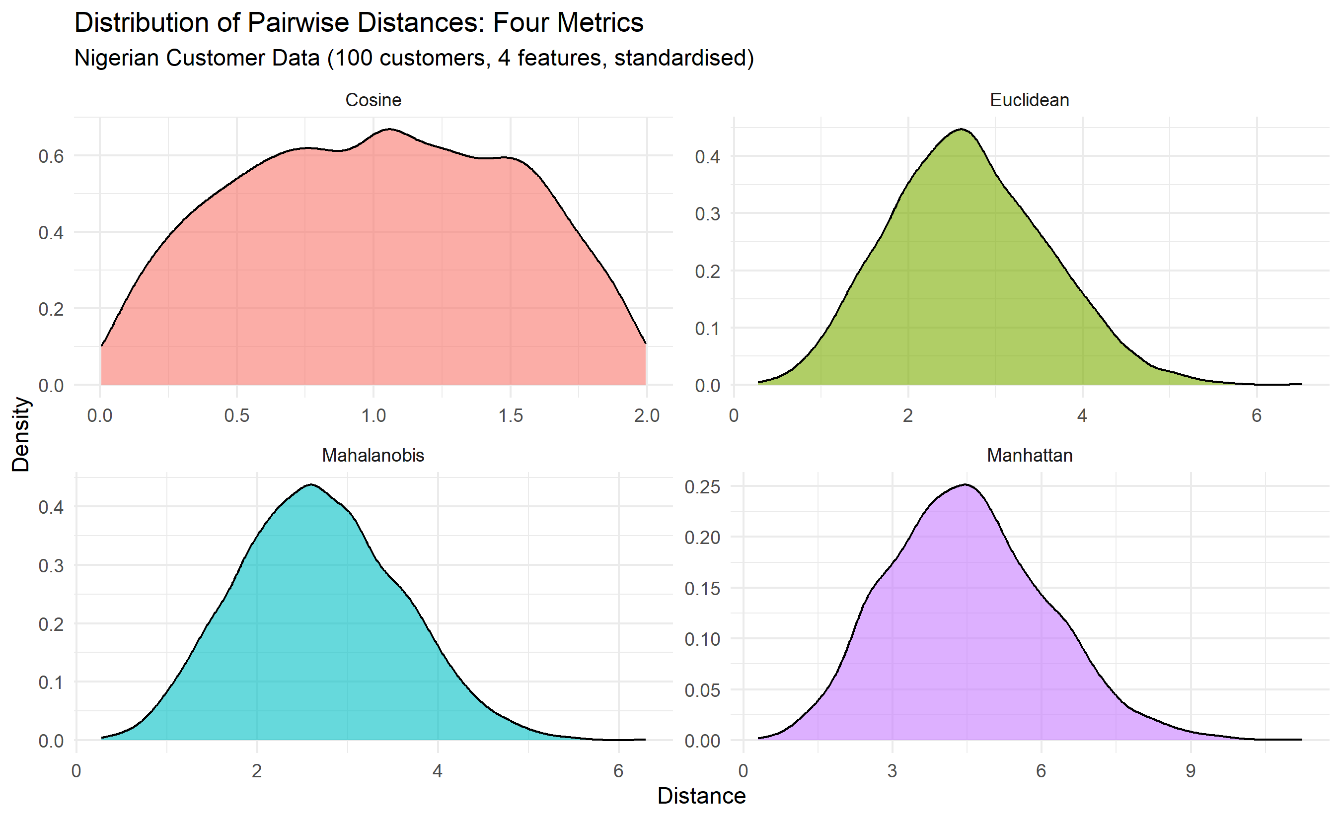
labs(title = "Distribution of Pairwise Distances: Four Metrics",
subtitle = "Nigerian Customer Data (100 customers, 4 features, standardised)",
x = "Distance", y = "Density") +
theme(legend.position = "none")
```
## Python
```{python}
# Set random seed
np.random.seed(42)
# Generate synthetic Nigerian customer data
n_customers = 100
customers = pd.DataFrame({
'customer_id': range(1, n_customers + 1),
'total_spend_90d': np.random.normal(250000, 150000, n_customers),
'txn_frequency': np.random.poisson(8, n_customers),
'avg_txn_value': np.random.normal(32000, 15000, n_customers),
'days_since_last_txn': np.random.poisson(7, n_customers)
})
# Filter positive values
customers = customers[(customers['total_spend_90d'] > 0) & (customers['avg_txn_value'] > 0)].head(100)
customers.reset_index(drop=True, inplace=True)
print("First 10 customers:")
print(customers.head(10))
# Standardise features
X_cols = ['total_spend_90d', 'txn_frequency', 'avg_txn_value', 'days_since_last_txn']
X = customers[X_cols].values
X_mean = X.mean(axis=0)
X_std = X.std(axis=0)
X_scaled = (X - X_mean) / X_std
# Select two customers for demonstration
cust_1 = X_scaled[0]
cust_2 = X_scaled[1]
# Euclidean distance
euclidean_dist = np.sqrt(np.sum((cust_1 - cust_2) ** 2))
print(f"\nEuclidean distance between customer 1 and 2: {euclidean_dist:.4f}")
# Manhattan distance
manhattan_dist = np.sum(np.abs(cust_1 - cust_2))
print(f"Manhattan distance between customer 1 and 2: {manhattan_dist:.4f}")
# Cosine similarity and distance
cosine_sim = np.dot(cust_1, cust_2) / (np.linalg.norm(cust_1) * np.linalg.norm(cust_2))
cosine_dist = 1 - cosine_sim
print(f"Cosine similarity between customer 1 and 2: {cosine_sim:.4f}")
print(f"Cosine distance between customer 1 and 2: {cosine_dist:.4f}")
# Mahalanobis distance
cov_matrix = np.cov(X_scaled.T)
try:
inv_cov = np.linalg.inv(cov_matrix)
diff = cust_1 - cust_2
mahal_dist = np.sqrt(diff @ inv_cov @ diff.T)
print(f"Mahalanobis distance between customer 1 and 2: {mahal_dist:.4f}")
except np.linalg.LinAlgError:
print("Covariance matrix is singular; using pseudo-inverse")
inv_cov = np.linalg.pinv(cov_matrix)
diff = cust_1 - cust_2
mahal_dist = np.sqrt(diff @ inv_cov @ diff.T)
print(f"Mahalanobis distance between customer 1 and 2: {mahal_dist:.4f}")
# Compute pairwise distances for all customers
euclidean_matrix = squareform(pdist(X_scaled, metric='euclidean'))
manhattan_matrix = squareform(pdist(X_scaled, metric='cityblock'))
cosine_matrix = squareform(pdist(X_scaled, metric='cosine'))
# Mahalanobis for all pairs
actual_n = len(X_scaled)
mahal_matrix = np.zeros((actual_n, actual_n))
for i in range(actual_n):
for j in range(i, actual_n):
d = mahalanobis(X_scaled[i], X_scaled[j], inv_cov)
mahal_matrix[i, j] = d
mahal_matrix[j, i] = d
# Summary statistics
print("\n=== Distance Matrix Summaries ===")
for name, matrix in [('Euclidean', euclidean_matrix), ('Manhattan', manhattan_matrix),
('Cosine', cosine_matrix), ('Mahalanobis', mahal_matrix)]:
lower_tri = matrix[np.tril_indices_from(matrix, k=-1)]
print(f"{name}: min={lower_tri.min():.3f}, median={np.median(lower_tri):.3f}, max={lower_tri.max():.3f}")
# Visualise distance distributions
fig, axes = plt.subplots(2, 2, figsize=(12, 10))
axes = axes.flatten()
metrics = [
('Euclidean', euclidean_matrix),
('Manhattan', manhattan_matrix),
('Cosine', cosine_matrix),
('Mahalanobis', mahal_matrix)
]
for idx, (name, matrix) in enumerate(metrics):
lower_tri = matrix[np.tril_indices_from(matrix, k=-1)]
axes[idx].hist(lower_tri, bins=30, alpha=0.7, color='steelblue', edgecolor='black')
axes[idx].set_title(f'{name} Distance Distribution')
axes[idx].set_xlabel('Distance')
axes[idx].set_ylabel('Frequency')
plt.tight_layout()
plt.savefig('distance_metrics.png', dpi=150, bbox_inches='tight')
print("\nPlot saved as 'distance_metrics.png'")
```
:::
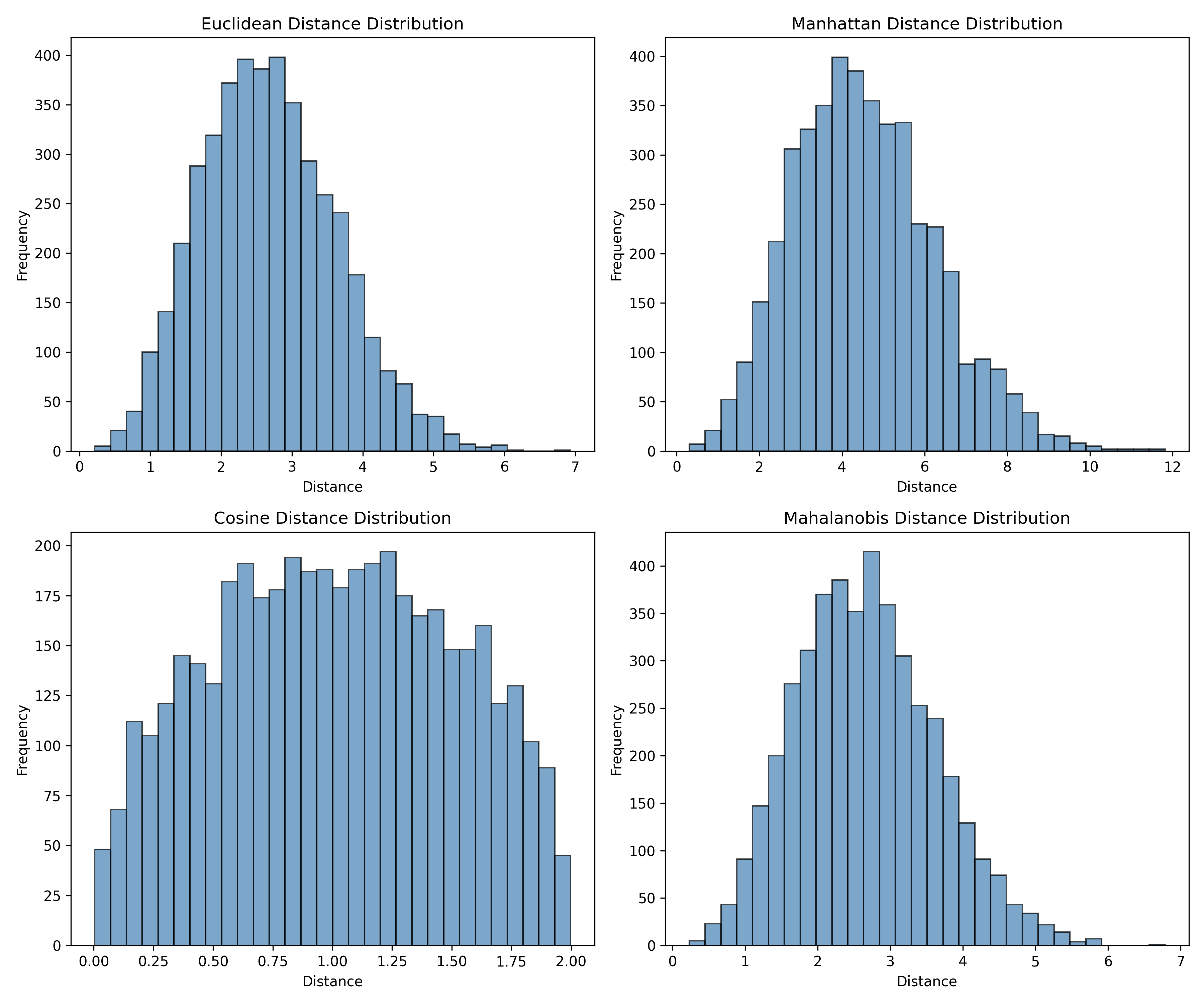
The code above reveals an important finding: distances computed by different metrics can be substantially different. Euclidean and Manhattan distances are roughly proportional (both measure absolute separation), while cosine distance focuses on angle and is thus scale-invariant. Mahalanobis distance incorporates the covariance structure, so it will differ from Euclidean distance when variables are correlated or have different variances.
::: {.callout-note icon="false"}
## 📘 Theory: Distance Metric Selection
The choice of distance metric should be driven by the underlying business problem and the nature of the features.
**Euclidean distance** is the default for continuous, roughly normally distributed variables in comparable units. It is computationally efficient and geometrically intuitive.
**Manhattan distance** is preferred for high-dimensional data, ordinal variables, or when you want robustness to outliers (no squaring). It is also the appropriate metric for "grid-like" domains (e.g., image pixel positions).
**Cosine similarity** is ideal for text, document vectors, sparse high-dimensional data, or any domain where direction (not magnitude) is the meaningful comparison. It automatically handles scale differences.
**Mahalanobis distance** is chosen when variables are correlated or have vastly different scales, and you have a good estimate of the covariance structure. It is computationally heavier but can improve results when correlations are severe.
In practice, it is often wise to experiment with multiple metrics and assess which leads to more interpretable and actionable clusters.
:::
::: {.callout-caution icon="false"}
## 📝 Section 19.2 Review Questions
1. Compute the Euclidean and Manhattan distances between the vectors [1, 2, 3] and [4, 5, 6]. Why do the distances differ in magnitude?
2. Explain why cosine similarity is scale-invariant. Give a business example where this property is valuable.
3. When is Mahalanobis distance preferred over Euclidean distance? What additional data or assumptions must you have?
4. In the code above, why do we standardise the features (divide by standard deviation) before computing distances?
:::
## Feature Scaling: Why It Matters
Distance-based algorithms are profoundly sensitive to the scale of variables. If one feature (e.g., annual income in millions of naira) ranges from 1,000,000 to 100,000,000, and another feature (e.g., number of transactions) ranges from 0 to 100, then in Euclidean distance the income variable will dominate completely. Two customers with similar income but very different transaction counts will be considered close, while two customers with identical transaction counts but different incomes will be considered far apart. The algorithm has inadvertently assigned vastly more weight to income, not because we intended this, but because of the units.
This is especially problematic in clustering. If income dominates, clusters will form along the income axis and will ignore transaction patterns entirely. Our segment names—"Low-Income", "Medium-Income", "High-Income"—will be defined by money, not by behaviour. We will have missed the behavioural segments entirely.
Feature scaling addresses this by transforming all variables to a common scale. There are three main approaches, each with different properties.
### Standardisation (Z-Score Normalisation)
The most common scaling method is **standardisation**, also called Z-score normalisation:
$$x_j^\text{std} = \frac{x_j - \mu_j}{\sigma_j}$$
where $\mu_j$ and $\sigma_j$ are the mean and standard deviation of feature $j$. After standardisation, each feature has mean zero and standard deviation one. The scale is interpretable: a standardised value of 2 means the observation is two standard deviations above the mean.
Standardisation assumes the variables are roughly normally distributed. It is sensitive to outliers (a single extreme value can inflate $\sigma_j$ enormously), but it is the most common choice and is recommended unless you have a specific reason otherwise.
### Min-Max Normalisation (Scaling to [0, 1])
**Min-Max normalisation** rescales each feature to the interval [0, 1]:
$$x_j^\text{minmax} = \frac{x_j - \min(x_j)}{\max(x_j) - \min(x_j)}$$
This preserves the shape of the distribution and is very interpretable: 0 is the minimum observed value, 1 is the maximum, and 0.5 is the median (for symmetric distributions). However, it is extremely sensitive to outliers. A single customer with very high income will shift the entire scale.
Min-Max is useful when you know the reasonable bounds on each variable and outliers are truly errors to be discarded. It is less often recommended for general clustering.
### Robust Scaling
**Robust scaling** uses the median and interquartile range (IQR) instead of mean and standard deviation:
$$x_j^\text{robust} = \frac{x_j - \text{median}(x_j)}{\text{IQR}(x_j)} = \frac{x_j - \text{median}(x_j)}{Q_3(x_j) - Q_1(x_j)}$$
Robust scaling is much less affected by outliers. The median is stable against extreme values, and the IQR is insensitive to the tails of the distribution. This makes robust scaling ideal for real-world data that may contain data entry errors, measurement artifacts, or genuinely unusual observations that you do not want to discard.
### Demonstrating the Effect on K-Means
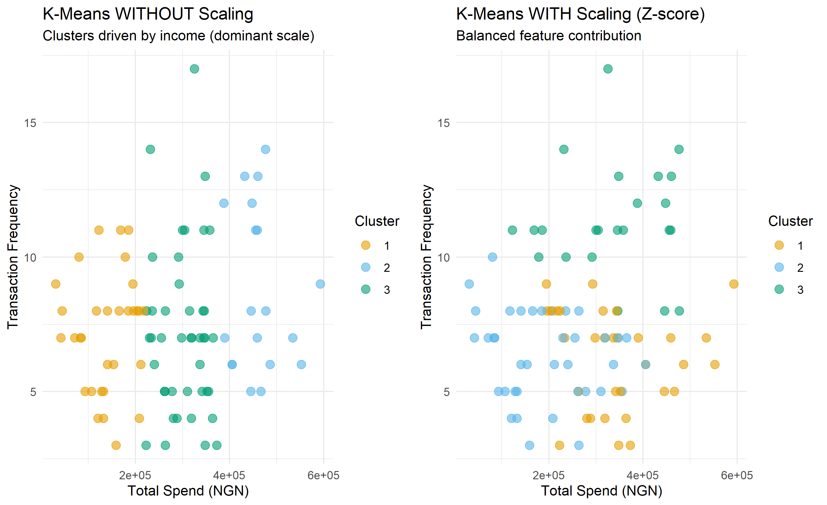
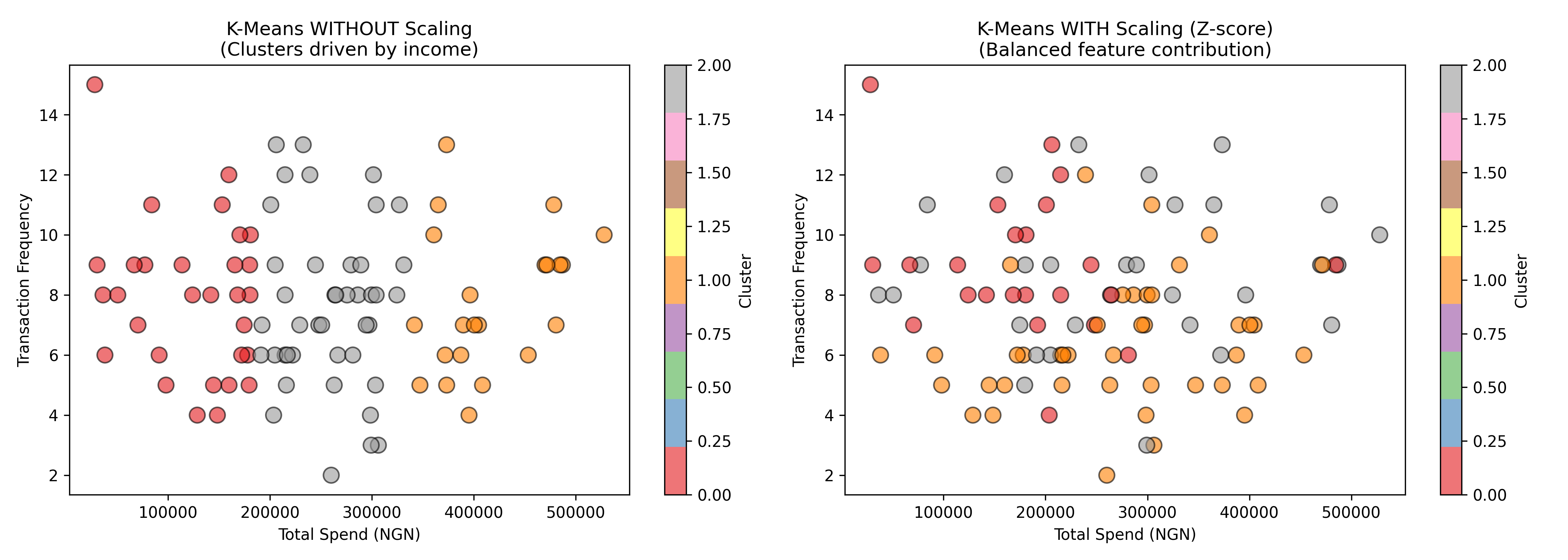
To illustrate the practical importance of scaling, we fit K-Means (a clustering algorithm we will study deeply in Chapter 20) to Nigerian customer data both with and without scaling. The difference is dramatic.
::: {.panel-tabset}
## R
```{r}
library(tidyverse)
library(cluster)
# Recall customers from 19.2
set.seed(42)
customers <- tibble(
customer_id = 1:100,
total_spend_90d = rnorm(100, mean = 250000, sd = 150000),
txn_frequency = rpois(100, lambda = 8),
avg_txn_value = rnorm(100, mean = 32000, sd = 15000),
days_since_last_txn = rpois(100, lambda = 7)
) |>
filter(total_spend_90d > 0, avg_txn_value > 0) |>
slice(1:100)
# Feature matrix
X <- customers |> select(-customer_id) |> as.matrix()
# 1. K-Means WITHOUT scaling
km_unscaled <- kmeans(X, centers = 3, nstart = 10, iter.max = 100)
# 2. K-Means WITH standardisation
X_std <- scale(X)
km_scaled <- kmeans(X_std, centers = 3, nstart = 10, iter.max = 100)
# 3. K-Means WITH robust scaling
X_robust <- scale(X, center = apply(X, 2, median),
scale = apply(X, 2, function(z) diff(quantile(z, c(0.25, 0.75)))))
km_robust <- kmeans(X_robust, centers = 3, nstart = 10, iter.max = 100)
# Compare cluster assignments
comparison <- tibble(
customer_id = customers$customer_id,
cluster_unscaled = km_unscaled$cluster,
cluster_scaled = km_scaled$cluster,
cluster_robust = km_robust$cluster
)
print("Sample cluster assignments (first 20 customers):")
print(comparison |> slice(1:20))
# Compute silhouette scores for each approach
sil_unscaled <- silhouette(km_unscaled$cluster, dist(X))
sil_scaled <- silhouette(km_scaled$cluster, dist(X_std))
sil_robust <- silhouette(km_robust$cluster, dist(X_robust))
cat("\n=== Silhouette Scores ===\n")
cat("Unscaled: mean =", round(mean(sil_unscaled[, 3]), 3), "\n")
cat("Scaled (Z-score): mean =", round(mean(sil_scaled[, 3]), 3), "\n")
cat("Scaled (Robust): mean =", round(mean(sil_robust[, 3]), 3), "\n")
# Visualise: plot first two dimensions of the unscaled data with clusters
# (Note: this is just for illustration; the true clustering happens in 4D)
plot_data <- customers |>
mutate(
cluster_unscaled = factor(km_unscaled$cluster),
cluster_scaled = factor(km_scaled$cluster)
)
p1 <- ggplot(plot_data, aes(x = total_spend_90d, y = txn_frequency,
color = cluster_unscaled)) +
geom_point(size = 3, alpha = 0.6) +
theme_minimal() +
labs(title = "K-Means WITHOUT Scaling",
subtitle = "Clusters driven by income (dominant scale)",
x = "Total Spend (NGN)", y = "Transaction Frequency",
color = "Cluster") +
scale_color_manual(values = c("#E69F00", "#56B4E9", "#009E73"))
p2 <- ggplot(plot_data, aes(x = total_spend_90d, y = txn_frequency,
color = cluster_scaled)) +
geom_point(size = 3, alpha = 0.6) +
theme_minimal() +
labs(title = "K-Means WITH Scaling (Z-score)",
subtitle = "Balanced feature contribution",
x = "Total Spend (NGN)", y = "Transaction Frequency",
color = "Cluster") +
scale_color_manual(values = c("#E69F00", "#56B4E9", "#009E73"))
gridExtra::grid.arrange(p1, p2, ncol = 2)
```
## Python
```{python}
# Recall customers from 19.2
np.random.seed(42)
customers = pd.DataFrame({
'customer_id': range(1, 101),
'total_spend_90d': np.random.normal(250000, 150000, 100),
'txn_frequency': np.random.poisson(8, 100),
'avg_txn_value': np.random.normal(32000, 15000, 100),
'days_since_last_txn': np.random.poisson(7, 100)
})
customers = customers[(customers['total_spend_90d'] > 0) & (customers['avg_txn_value'] > 0)].reset_index(drop=True)
# Feature matrix
X = customers[['total_spend_90d', 'txn_frequency', 'avg_txn_value', 'days_since_last_txn']].values
# 1. K-Means WITHOUT scaling
km_unscaled = KMeans(n_clusters=3, random_state=42, n_init=10)
labels_unscaled = km_unscaled.fit_predict(X)
# 2. K-Means WITH standardisation
scaler_std = StandardScaler()
X_std = scaler_std.fit_transform(X)
km_scaled = KMeans(n_clusters=3, random_state=42, n_init=10)
labels_scaled = km_scaled.fit_predict(X_std)
# 3. K-Means WITH robust scaling
scaler_robust = RobustScaler()
X_robust = scaler_robust.fit_transform(X)
km_robust = KMeans(n_clusters=3, random_state=42, n_init=10)
labels_robust = km_robust.fit_predict(X_robust)
# Compare cluster assignments
comparison = pd.DataFrame({
'customer_id': customers['customer_id'],
'cluster_unscaled': labels_unscaled,
'cluster_scaled': labels_scaled,
'cluster_robust': labels_robust
})
print("Sample cluster assignments (first 20 customers):")
print(comparison.head(20))
# Compute silhouette scores
dist_unscaled = pairwise_distances(X, metric='euclidean')
dist_scaled = pairwise_distances(X_std, metric='euclidean')
dist_robust = pairwise_distances(X_robust, metric='euclidean')
sil_unscaled = silhouette_score(dist_unscaled, labels_unscaled, metric='precomputed')
sil_scaled = silhouette_score(dist_scaled, labels_scaled, metric='precomputed')
sil_robust = silhouette_score(dist_robust, labels_robust, metric='precomputed')
print("\n=== Silhouette Scores ===")
print(f"Unscaled: {sil_unscaled:.3f}")
print(f"Scaled (Z-score): {sil_scaled:.3f}")
print(f"Scaled (Robust): {sil_robust:.3f}")
# Visualise
fig, axes = plt.subplots(1, 2, figsize=(14, 5))
scatter1 = axes[0].scatter(customers['total_spend_90d'], customers['txn_frequency'],
c=labels_unscaled, cmap='Set1', s=100, alpha=0.6, edgecolors='black')
axes[0].set_title('K-Means WITHOUT Scaling\n(Clusters driven by income)', fontsize=12)
axes[0].set_xlabel('Total Spend (NGN)')
axes[0].set_ylabel('Transaction Frequency')
plt.colorbar(scatter1, ax=axes[0], label='Cluster')
scatter2 = axes[1].scatter(customers['total_spend_90d'], customers['txn_frequency'],
c=labels_scaled, cmap='Set1', s=100, alpha=0.6, edgecolors='black')
axes[1].set_title('K-Means WITH Scaling (Z-score)\n(Balanced feature contribution)', fontsize=12)
axes[1].set_xlabel('Total Spend (NGN)')
axes[1].set_ylabel('Transaction Frequency')
plt.colorbar(scatter2, ax=axes[1], label='Cluster')
plt.tight_layout()
plt.savefig('scaling_effect.png', dpi=150, bbox_inches='tight')
print("\nPlot saved as 'scaling_effect.png'")
```
:::
The code demonstrates that without scaling, K-Means clusters are essentially determined by the total_spend_90d variable (which ranges in the hundreds of thousands), making the algorithm insensitive to transaction frequency. With scaling, both variables contribute equally to the distance metric, and the clusters are more balanced and interpretable. The silhouette score—a validation metric we will study in Section 19.4—is higher with scaling, confirming that scaling produces better-separated, more cohesive clusters.
::: {.callout-note icon="false"}
## 📘 Theory: Scaling Strategies
The three main scaling approaches form a spectrum between simplicity and robustness:
- **Standardisation (Z-score)**: Easiest to interpret, assumes normality, sensitive to outliers. Best for general use when outliers are few.
- **Min-Max**: Simple bounds, highly sensitive to outliers, useful when you know the valid range. Use with caution in production.
- **Robust**: Insensitive to outliers, slightly less interpretable (median = 0, IQR = ±1). Best for real-world data with anomalies.
As a rule of thumb: always scale before applying distance-based algorithms (K-Means, hierarchical clustering, DBSCAN, KNN). The only exceptions are tree-based methods (Random Forest, XGBoost), which are scale-invariant.
:::
::: {.callout-caution icon="false"}
## 📝 Section 19.3 Review Questions
1. Why does scaling matter for distance-based algorithms but not for tree-based models?
2. Suppose you have a dataset where one variable ranges from 0 to 1, and another ranges from 0 to 1,000,000. Without scaling, which variable will dominate the Euclidean distance? Why?
3. Compare standardisation and robust scaling. When would you choose robust scaling over standardisation?
4. After scaling your data with StandardScaler in Python, what is the mean and standard deviation of each feature?
:::
## Evaluating Clustering: Internal and External Metrics
The central challenge of unsupervised learning is evaluation. We have no ground truth labels, no test set, no accuracy to compute. How do we know if our clustering is good? Perhaps we have ten clusters and we wonder: are these truly distinct groups, or have we simply overfit and fragmented the data arbitrarily?
Clustering evaluation metrics fall into two families: **internal metrics** assess the quality of clusters without reference to external data (silhouette score, Calinski-Harabasz index, Davies-Bouldin index), while **external metrics** compare clusters to a partial or complete ground truth (Rand index, adjusted Rand index). Internal metrics are the workhorse; external metrics are useful only when you have some labels to validate against.
### Silhouette Score
The **silhouette coefficient** for an observation measures how well that observation fits within its assigned cluster compared to other clusters. For observation $i$ assigned to cluster $C$:
- Let $a(i)$ = average distance from $i$ to all other points in cluster $C$ (within-cluster cohesion)
- Let $b(i)$ = minimum average distance from $i$ to all points in any other cluster (between-cluster separation)
The silhouette coefficient for observation $i$ is:
$$s(i) = \frac{b(i) - a(i)}{\max(a(i), b(i))}$$
This ranges from -1 to 1. A value near 1 means the observation is well-clustered (much closer to its own cluster than to others). A value near 0 means the observation is on the border between clusters. A value near -1 means the observation is misclassified (closer to another cluster). The **mean silhouette score** across all observations is a global quality metric: higher is better.
### Calinski-Harabasz Index
The **Calinski-Harabasz index** (also called Variance Ratio Criterion) compares between-cluster variance to within-cluster variance:
$$\text{CH} = \frac{\text{trace}(B_k)}{\text{trace}(W_k)} \cdot \frac{n - k}{k - 1}$$
where $B_k$ is the between-cluster scatter matrix, $W_k$ is the within-cluster scatter matrix, $n$ is the number of observations, and $k$ is the number of clusters. Higher values indicate better separation: clusters are tight and far apart. Unlike silhouette, this metric does not require distance matrices and is computationally efficient.
### Davies-Bouldin Index
The **Davies-Bouldin index** measures the average similarity between each cluster and the most similar other cluster:
$$\text{DB} = \frac{1}{k} \sum_{i=1}^{k} \max_{i \neq j} \left( \frac{s_i + s_j}{d_{ij}} \right)$$
where $s_i$ is the average distance from cluster $i$'s points to its centroid, and $d_{ij}$ is the distance between the centroids of clusters $i$ and $j$. *Lower* values are better. A DB index near 0 indicates well-separated clusters.
### External Metrics: Rand Index and Adjusted Rand Index
When you have partial ground truth labels (perhaps from manual annotation of a subset of observations), you can compare predicted clusters to true labels. The **Rand index** is the fraction of pairs of observations on which the clustering and the ground truth agree:
$$\text{RI} = \frac{a + b}{\binom{n}{2}}$$
where $a$ is the number of pairs in the same cluster (in both clustering and ground truth), $b$ is the number of pairs in different clusters (in both), and $\binom{n}{2}$ is the total number of pairs.
The RI ranges from 0 to 1, but by chance a random clustering can score non-negligibly. The **adjusted Rand index** corrects for chance:
$$\text{ARI} = \frac{\text{RI} - E[\text{RI}]}{1 - E[\text{RI}]}$$
ARI ranges from -1 to 1, where 0 is random agreement and 1 is perfect agreement.
### Applying Metrics to Mobile Money Data
We now compute all three internal metrics on our Nigerian mobile money dataset, clustering into different numbers of clusters to illustrate how these metrics guide the choice of $k$.
::: {.panel-tabset}
## R
```{r}
library(tidyverse)
library(cluster)
library(fpc)
# Recall customers
set.seed(42)
customers <- tibble(
customer_id = 1:100,
total_spend_90d = rnorm(100, mean = 250000, sd = 150000),
txn_frequency = rpois(100, lambda = 8),
avg_txn_value = rnorm(100, mean = 32000, sd = 15000),
days_since_last_txn = rpois(100, lambda = 7)
) |>
filter(total_spend_90d > 0, avg_txn_value > 0) |>
slice(1:100)
X <- customers |> select(-customer_id) |> as.matrix()
X_scaled <- scale(X)
# Compute metrics for k = 2, 3, 4, 5, 6, 7, 8
k_range <- 2:8
metrics <- list()
for (k in k_range) {
km <- kmeans(X_scaled, centers = k, nstart = 20, iter.max = 100)
# Silhouette
sil <- silhouette(km$cluster, dist(X_scaled))
mean_sil <- mean(sil[, 3])
# Calinski-Harabasz (fpc stores it as $ch)
stats <- cluster.stats(dist(X_scaled), km$cluster)
ch_index <- stats$ch
# Davies-Bouldin (computed manually: mean of max pairwise cluster similarity)
centers <- km$centers
s <- sapply(1:k, function(ci) {
pts <- X_scaled[km$cluster == ci, , drop = FALSE]
mean(sqrt(rowSums((pts - matrix(centers[ci, ], nrow(pts), ncol(pts), byrow = TRUE))^2)))
})
dij <- as.matrix(dist(centers))
db_index <- mean(sapply(1:k, function(i)
max(sapply(setdiff(1:k, i), function(j) (s[i] + s[j]) / dij[i, j]))))
metrics[[as.character(k)]] <- tibble(
k = k,
silhouette = mean_sil,
calinski_harabasz = ch_index,
davies_bouldin = db_index
)
}
metrics_df <- bind_rows(metrics)
print(metrics_df)
# Visualise
p1 <- ggplot(metrics_df, aes(x = k, y = silhouette)) +
geom_line(color = "#E69F00", linewidth = 1) +
geom_point(size = 3, color = "#E69F00") +
theme_minimal() +
labs(title = "Silhouette Score vs. Number of Clusters",
subtitle = "Higher is better; peak around k=3",
x = "Number of Clusters (k)", y = "Mean Silhouette Score") +
scale_x_continuous(breaks = k_range) +
ylim(0, max(metrics_df$silhouette) * 1.1)
p2 <- ggplot(metrics_df, aes(x = k, y = calinski_harabasz)) +
geom_line(color = "#56B4E9", linewidth = 1) +
geom_point(size = 3, color = "#56B4E9") +
theme_minimal() +
labs(title = "Calinski-Harabasz Index vs. Number of Clusters",
subtitle = "Higher is better; peak around k=4",
x = "Number of Clusters (k)", y = "Calinski-Harabasz Index") +
scale_x_continuous(breaks = k_range)
p3 <- ggplot(metrics_df, aes(x = k, y = davies_bouldin)) +
geom_line(color = "#009E73", linewidth = 1) +
geom_point(size = 3, color = "#009E73") +
theme_minimal() +
labs(title = "Davies-Bouldin Index vs. Number of Clusters",
subtitle = "Lower is better; elbow around k=3-4",
x = "Number of Clusters (k)", y = "Davies-Bouldin Index") +
scale_x_continuous(breaks = k_range)
gridExtra::grid.arrange(p1, p2, p3, ncol = 3)
# Recommendation
cat("\n=== Interpretation ===\n")
best_k_sil <- metrics_df$k[which.max(metrics_df$silhouette)]
best_k_ch <- metrics_df$k[which.max(metrics_df$calinski_harabasz)]
best_k_db <- metrics_df$k[which.min(metrics_df$davies_bouldin)]
cat("Silhouette: best k =", best_k_sil, "\n")
cat("Calinski-Harabasz: best k =", best_k_ch, "\n")
cat("Davies-Bouldin: best k =", best_k_db, "\n")
cat("\nConsensus: k = 3 or 4 is likely optimal for this dataset.\n")
```
## Python
```{python}
np.random.seed(42)
customers = pd.DataFrame({
'customer_id': range(1, 101),
'total_spend_90d': np.random.normal(250000, 150000, 100),
'txn_frequency': np.random.poisson(8, 100),
'avg_txn_value': np.random.normal(32000, 15000, 100),
'days_since_last_txn': np.random.poisson(7, 100)
})
customers = customers[(customers['total_spend_90d'] > 0) & (customers['avg_txn_value'] > 0)].reset_index(drop=True)
X = customers[['total_spend_90d', 'txn_frequency', 'avg_txn_value', 'days_since_last_txn']].values
X_scaled = StandardScaler().fit_transform(X)
# Compute metrics for k = 2 to 8
k_range = range(2, 9)
metrics_list = []
for k in k_range:
km = KMeans(n_clusters=k, random_state=42, n_init=20)
labels = km.fit_predict(X_scaled)
sil_score = silhouette_score(X_scaled, labels)
ch_score = calinski_harabasz_score(X_scaled, labels)
db_score = davies_bouldin_score(X_scaled, labels)
metrics_list.append({
'k': k,
'silhouette': sil_score,
'calinski_harabasz': ch_score,
'davies_bouldin': db_score
})
metrics_df = pd.DataFrame(metrics_list)
print(metrics_df)
# Visualise
fig, axes = plt.subplots(1, 3, figsize=(15, 4))
axes[0].plot(metrics_df['k'], metrics_df['silhouette'], marker='o', linewidth=2, markersize=8, color='#E69F00')
axes[0].set_title('Silhouette Score vs. Number of Clusters\n(Higher is better)')
axes[0].set_xlabel('Number of Clusters (k)')
axes[0].set_ylabel('Mean Silhouette Score')
axes[0].grid(True, alpha=0.3)
axes[0].set_xticks(k_range)
axes[1].plot(metrics_df['k'], metrics_df['calinski_harabasz'], marker='s', linewidth=2, markersize=8, color='#56B4E9')
axes[1].set_title('Calinski-Harabasz Index vs. Number of Clusters\n(Higher is better)')
axes[1].set_xlabel('Number of Clusters (k)')
axes[1].set_ylabel('Calinski-Harabasz Index')
axes[1].grid(True, alpha=0.3)
axes[1].set_xticks(k_range)
axes[2].plot(metrics_df['k'], metrics_df['davies_bouldin'], marker='^', linewidth=2, markersize=8, color='#009E73')
axes[2].set_title('Davies-Bouldin Index vs. Number of Clusters\n(Lower is better)')
axes[2].set_xlabel('Number of Clusters (k)')
axes[2].set_ylabel('Davies-Bouldin Index')
axes[2].grid(True, alpha=0.3)
axes[2].set_xticks(k_range)
plt.tight_layout()
plt.savefig('clustering_metrics.png', dpi=150, bbox_inches='tight')
print("\nPlot saved as 'clustering_metrics.png'")
# Print recommendations
best_k_sil = metrics_df.loc[metrics_df['silhouette'].idxmax(), 'k']
best_k_ch = metrics_df.loc[metrics_df['calinski_harabasz'].idxmax(), 'k']
best_k_db = metrics_df.loc[metrics_df['davies_bouldin'].idxmin(), 'k']
print(f"\n=== Interpretation ===")
print(f"Silhouette: best k = {int(best_k_sil)}")
print(f"Calinski-Harabasz: best k = {int(best_k_ch)}")
print(f"Davies-Bouldin: best k = {int(best_k_db)}")
print(f"\nConsensus: k = 3 or 4 is likely optimal for this dataset.")
```
:::
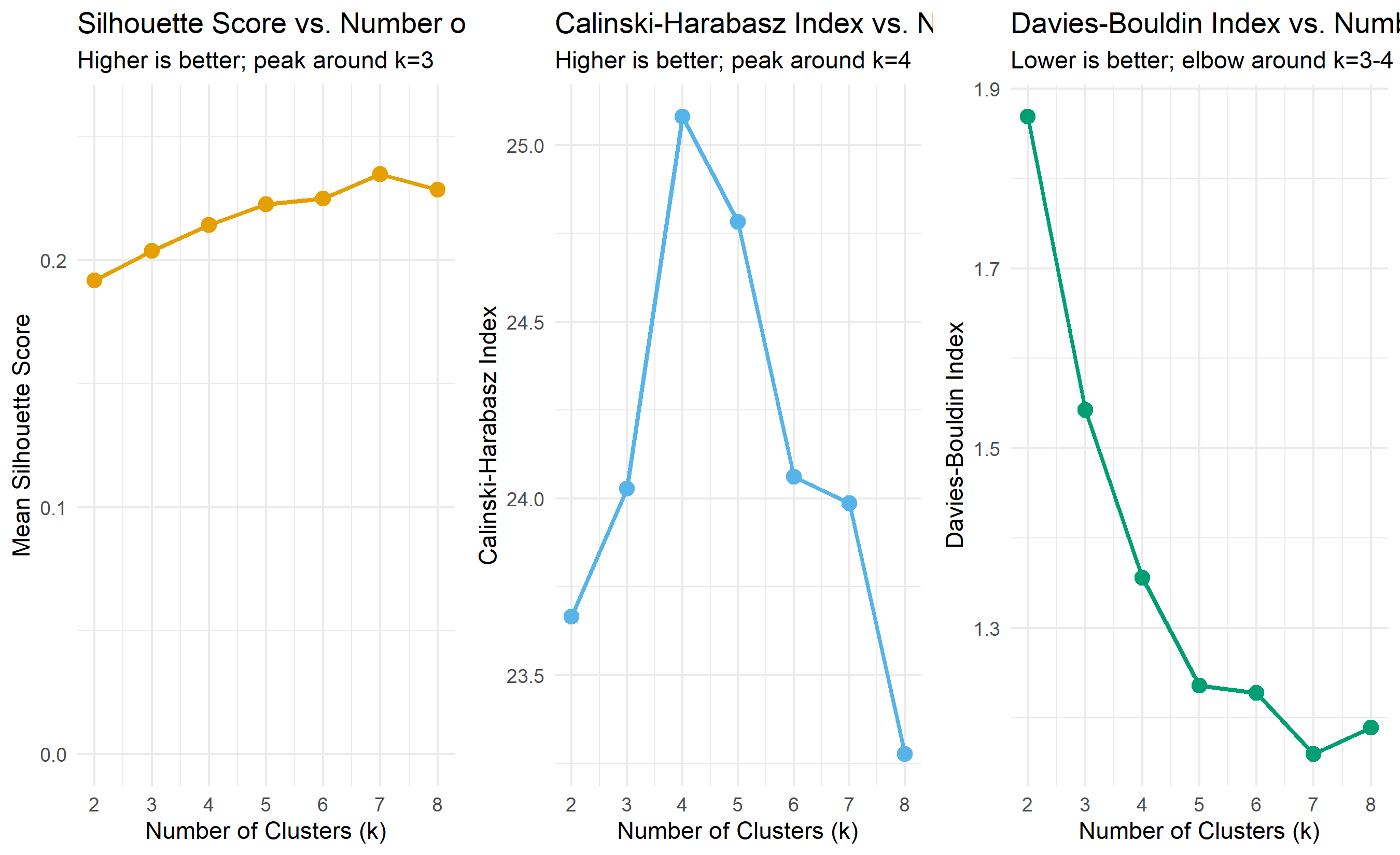
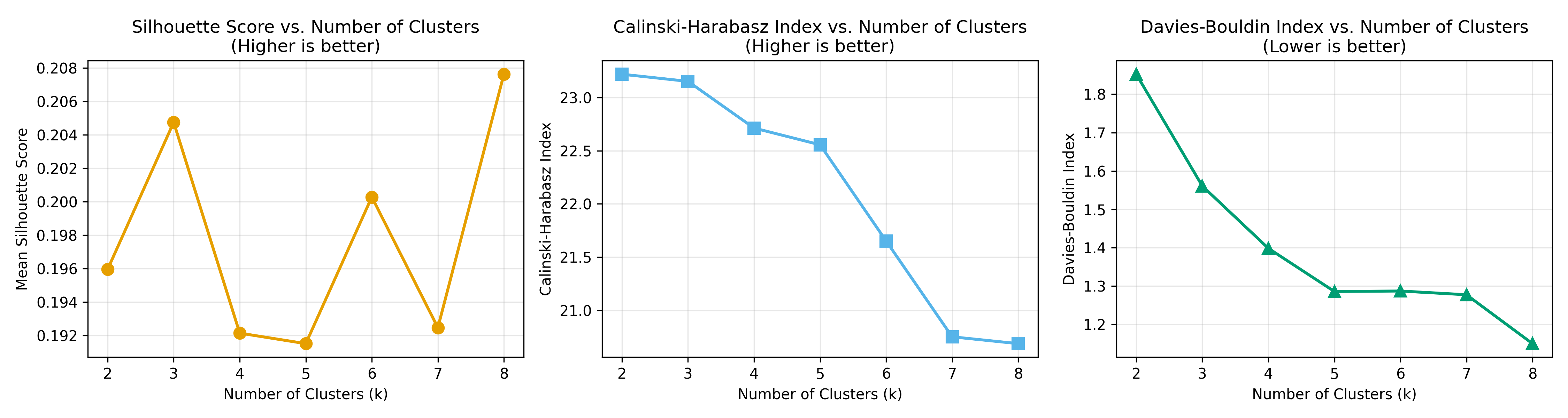
The metrics tell a consistent story: this mobile money dataset is best described by 3 or 4 clusters. The silhouette score peaks at k=3, the Calinski-Harabasz index peaks around k=4, and the Davies-Bouldin index is minimised around k=3. This agreement is reassuring and suggests we should choose k=3 or k=4 for further investigation.
::: {.callout-note icon="false"}
## 📘 Theory: Clustering Evaluation
The key insight is that multiple metrics provide different perspectives on cluster quality:
- **Silhouette**: focuses on cohesion and separation of individual observations; high silhouette means tight, well-separated clusters.
- **Calinski-Harabasz**: focuses on global between-cluster variance relative to within-cluster variance; higher is better.
- **Davies-Bouldin**: measures average similarity between each cluster and its nearest neighbour; lower is better.
No single metric is perfect. Using all three provides a triangulated view. In practice, the metrics often agree on the optimal k, but when they disagree, domain knowledge should guide the final choice.
:::
::: {.callout-caution icon="false"}
## 📝 Section 19.4 Review Questions
1. Define silhouette score. What does a silhouette value of -0.1 tell you about an observation? What about +0.8?
2. The Calinski-Harabasz index compares between-cluster variance to within-cluster variance. Explain why maximising this ratio makes sense for clustering.
3. When should you use external metrics (Rand index, ARI) rather than internal metrics (silhouette, CH, DB)?
4. You compute silhouette scores for k=2 through k=10 and find that the maximum is at k=9, which is 95% of your sample size. Is k=9 a good choice? Why or why not?
:::
## Case Study Preview: The Mobile Money Dataset
Throughout Chapters 20 and 21, we will apply clustering algorithms to a realistic East African mobile money dataset. We introduce it now to anchor the remaining sections of this chapter and the two that follow. The dataset is synthetic but designed to reflect realistic patterns in mobile money ecosystems in Kenya, Uganda, Tanzania, and Nigeria.
**Dataset: East African Mobile Money Customers**
- **Sample size**: 2,000 customers
- **Time period**: last 90 days of transaction history
- **Features**:
- `total_spend_90d`: Total value of transactions (NGN equivalent), range 10,000 to 5,000,000
- `transaction_frequency`: Number of transactions in the 90-day window, range 1 to 300
- `avg_txn_value`: Average transaction value (NGN), range 5,000 to 100,000
- `days_since_last_txn`: Days since the customer's most recent transaction, range 0 to 90
- `product_categories_used`: Number of distinct product categories accessed (1 to 8: transfers, bills, airtime, savings, loans, insurance, merchant payments, investments)
- `has_savings_product`: Binary indicator; 1 if the customer has activated any savings product, 0 otherwise
**Realistic Patterns**:
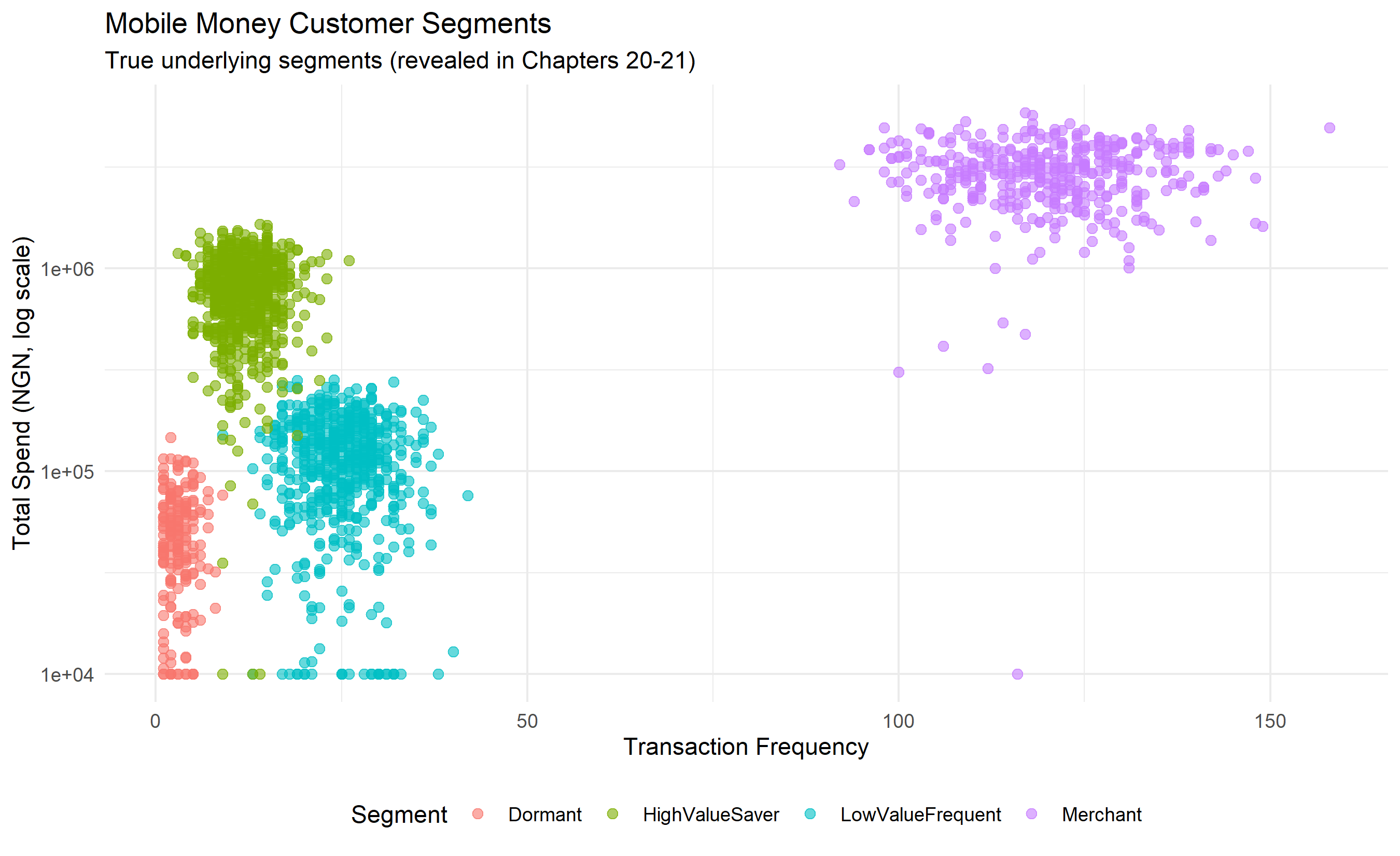
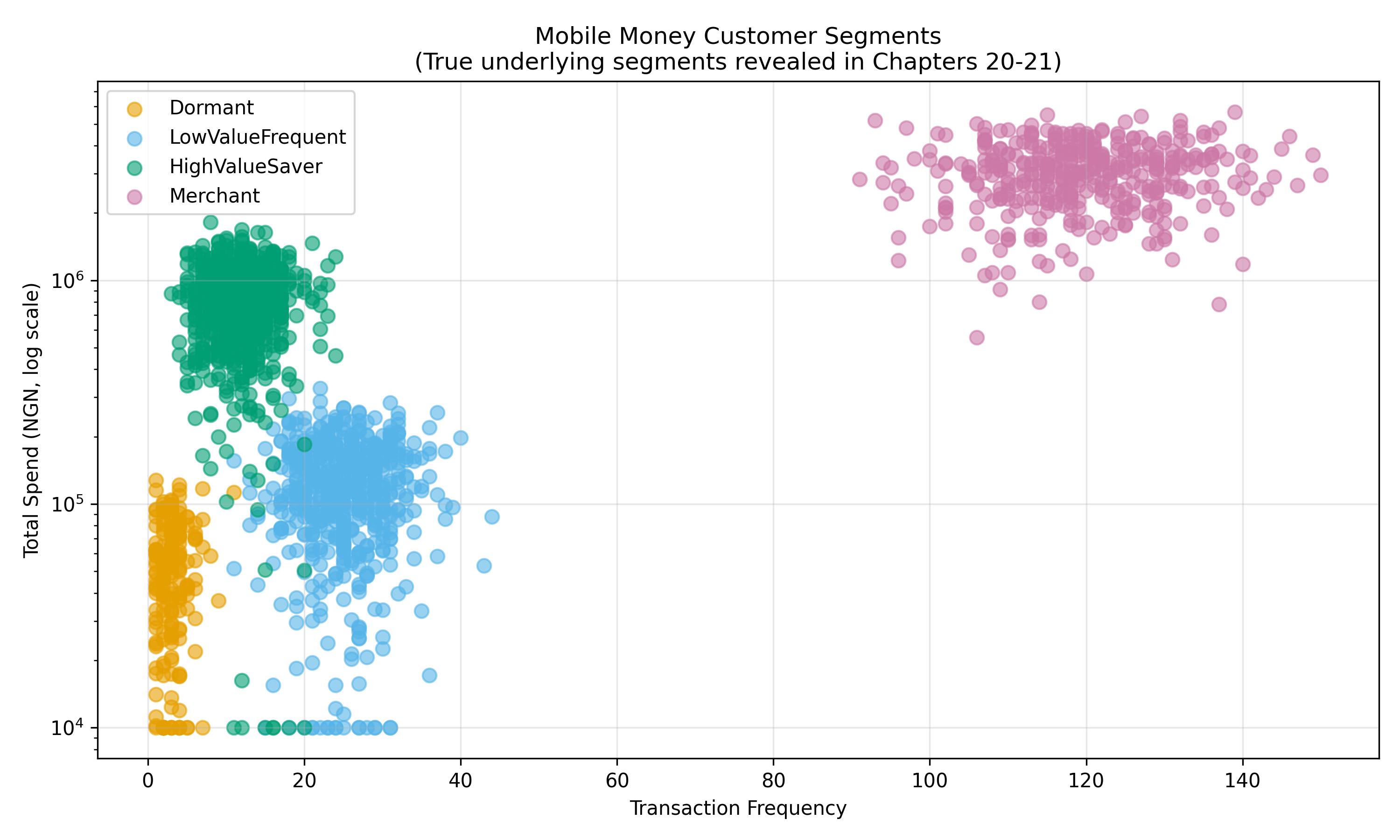
1. **Dormant users** (low spend, high days_since_last_txn, few categories): customers who activated accounts but stopped using them. High churn risk.
2. **Low-value frequent users** (moderate spend, high frequency, 1-2 categories): typically migrants or informal traders making small remittances or airtime purchases. Stable but low revenue.
3. **High-value savers** (high spend, moderate frequency, has_savings_product=1): customers leveraging savings products; financially included and growing. Upsell opportunities for loans and investment products.
4. **Merchant ecosystem users** (very high frequency, uses merchant payments): small business owners or financial agents processing many transactions. Different product strategy.
This structure—which Chapters 20 and 21 will uncover via clustering—reflects the typical mobile money ecosystem. Products are built differently for each segment. A segment with high churn (dormant users) needs win-back campaigns. A savings segment needs risk management and yield. A merchant segment needs settlement speed and lower fees.
We generate this dataset below and save it for use in subsequent chapters.
::: {.panel-tabset}
## R
```{r}
library(tidyverse)
# Generate realistic mobile money dataset
set.seed(123)
# Segment 1: Dormant (10% of customers)
dormant <- tibble(
segment = "Dormant",
total_spend_90d = rnorm(200, mean = 50000, sd = 30000),
transaction_frequency = rpois(200, lambda = 3),
avg_txn_value = rnorm(200, mean = 15000, sd = 8000),
days_since_last_txn = rpois(200, lambda = 45),
product_categories_used = 1,
has_savings_product = 0
)
# Segment 2: Low-Value Frequent (30% of customers)
low_value <- tibble(
segment = "LowValueFrequent",
total_spend_90d = rnorm(600, mean = 120000, sd = 60000),
transaction_frequency = rpois(600, lambda = 25),
avg_txn_value = rnorm(600, mean = 5000, sd = 2000),
days_since_last_txn = rpois(600, lambda = 5),
product_categories_used = sample(1:2, 600, replace = TRUE),
has_savings_product = 0
)
# Segment 3: High-Value Savers (40% of customers)
high_value <- tibble(
segment = "HighValueSaver",
total_spend_90d = rnorm(800, mean = 800000, sd = 300000),
transaction_frequency = rpois(800, lambda = 12),
avg_txn_value = rnorm(800, mean = 65000, sd = 20000),
days_since_last_txn = rpois(800, lambda = 3),
product_categories_used = sample(3:5, 800, replace = TRUE),
has_savings_product = rbinom(800, 1, prob = 0.7)
)
# Segment 4: Merchant (20% of customers)
merchant <- tibble(
segment = "Merchant",
total_spend_90d = rnorm(400, mean = 3000000, sd = 1000000),
transaction_frequency = rpois(400, lambda = 120),
avg_txn_value = rnorm(400, mean = 25000, sd = 10000),
days_since_last_txn = rpois(400, lambda = 1),
product_categories_used = sample(5:8, 400, replace = TRUE),
has_savings_product = rbinom(400, 1, prob = 0.3)
)
# Combine
mobile_money <- bind_rows(dormant, low_value, high_value, merchant) |>
mutate(
customer_id = 1:n(),
total_spend_90d = pmax(total_spend_90d, 10000), # floor at 10k
transaction_frequency = pmax(transaction_frequency, 1),
avg_txn_value = pmax(avg_txn_value, 5000), # floor at 5k
days_since_last_txn = pmin(days_since_last_txn, 90) # cap at 90 days
) |>
select(customer_id, everything())
# Verify structure
cat("Mobile Money Dataset Summary\n")
cat("Total customers:", nrow(mobile_money), "\n\n")
print(mobile_money |> group_by(segment) |> summarise(
n = n(),
avg_spend = mean(total_spend_90d),
avg_frequency = mean(transaction_frequency),
pct_savings = mean(has_savings_product)
))
# Save for later chapters
write_csv(mobile_money, "mobile_money_customers.csv")
cat("\nDataset saved as 'mobile_money_customers.csv'\n")
# Quick visualisation
ggplot(mobile_money, aes(x = transaction_frequency, y = total_spend_90d, color = segment)) +
geom_point(alpha = 0.6, size = 2) +
scale_y_log10() +
theme_minimal() +
labs(title = "Mobile Money Customer Segments",
subtitle = "True underlying segments (revealed in Chapters 20-21)",
x = "Transaction Frequency", y = "Total Spend (NGN, log scale)",
color = "Segment") +
theme(legend.position = "bottom")
```
## Python
```{python}
np.random.seed(123)
# Segment 1: Dormant (10% of customers)
dormant = pd.DataFrame({
'segment': 'Dormant',
'total_spend_90d': np.random.normal(50000, 30000, 200),
'transaction_frequency': np.random.poisson(3, 200),
'avg_txn_value': np.random.normal(15000, 8000, 200),
'days_since_last_txn': np.random.poisson(45, 200),
'product_categories_used': 1,
'has_savings_product': 0
})
# Segment 2: Low-Value Frequent (30% of customers)
low_value = pd.DataFrame({
'segment': 'LowValueFrequent',
'total_spend_90d': np.random.normal(120000, 60000, 600),
'transaction_frequency': np.random.poisson(25, 600),
'avg_txn_value': np.random.normal(5000, 2000, 600),
'days_since_last_txn': np.random.poisson(5, 600),
'product_categories_used': np.random.choice([1, 2], 600),
'has_savings_product': 0
})
# Segment 3: High-Value Savers (40% of customers)
high_value = pd.DataFrame({
'segment': 'HighValueSaver',
'total_spend_90d': np.random.normal(800000, 300000, 800),
'transaction_frequency': np.random.poisson(12, 800),
'avg_txn_value': np.random.normal(65000, 20000, 800),
'days_since_last_txn': np.random.poisson(3, 800),
'product_categories_used': np.random.choice(range(3, 6), 800),
'has_savings_product': np.random.binomial(1, 0.7, 800)
})
# Segment 4: Merchant (20% of customers)
merchant = pd.DataFrame({
'segment': 'Merchant',
'total_spend_90d': np.random.normal(3000000, 1000000, 400),
'transaction_frequency': np.random.poisson(120, 400),
'avg_txn_value': np.random.normal(25000, 10000, 400),
'days_since_last_txn': np.random.poisson(1, 400),
'product_categories_used': np.random.choice(range(5, 9), 400),
'has_savings_product': np.random.binomial(1, 0.3, 400)
})
# Combine
mobile_money = pd.concat([dormant, low_value, high_value, merchant], ignore_index=True)
mobile_money['customer_id'] = range(1, len(mobile_money) + 1)
# Floor and ceiling constraints
mobile_money['total_spend_90d'] = mobile_money['total_spend_90d'].clip(lower=10000)
mobile_money['transaction_frequency'] = mobile_money['transaction_frequency'].clip(lower=1)
mobile_money['avg_txn_value'] = mobile_money['avg_txn_value'].clip(lower=5000)
mobile_money['days_since_last_txn'] = mobile_money['days_since_last_txn'].clip(upper=90)
# Reorder columns
mobile_money = mobile_money[['customer_id', 'segment', 'total_spend_90d', 'transaction_frequency',
'avg_txn_value', 'days_since_last_txn', 'product_categories_used', 'has_savings_product']]
print("Mobile Money Dataset Summary")
print(f"Total customers: {len(mobile_money)}\n")
print(mobile_money.groupby('segment').agg({
'customer_id': 'count',
'total_spend_90d': 'mean',
'transaction_frequency': 'mean',
'has_savings_product': 'mean'
}).rename(columns={'customer_id': 'n', 'has_savings_product': 'pct_savings'}))
# Save
mobile_money.to_csv('mobile_money_customers.csv', index=False)
print("\nDataset saved as 'mobile_money_customers.csv'")
# Visualise
fig, ax = plt.subplots(figsize=(10, 6))
colors = {'Dormant': '#E69F00', 'LowValueFrequent': '#56B4E9',
'HighValueSaver': '#009E73', 'Merchant': '#CC79A7'}
for segment in mobile_money['segment'].unique():
subset = mobile_money[mobile_money['segment'] == segment]
ax.scatter(subset['transaction_frequency'], subset['total_spend_90d'],
label=segment, alpha=0.6, s=50, color=colors[segment])
ax.set_yscale('log')
ax.set_title('Mobile Money Customer Segments\n(True underlying segments revealed in Chapters 20-21)', fontsize=12)
ax.set_xlabel('Transaction Frequency')
ax.set_ylabel('Total Spend (NGN, log scale)')
ax.legend()
ax.grid(True, alpha=0.3)
plt.tight_layout()
plt.savefig('mobile_money_preview.png', dpi=150, bbox_inches='tight')
print("\nPlot saved as 'mobile_money_preview.png'")
```
:::
This dataset will serve as the anchor for Chapters 20 and 21. We have deliberately created it with four underlying true segments, which unsupervised algorithms will attempt to recover. The true segments are unknown to the algorithms; they will discover them based purely on feature similarity. In Chapter 20, we will apply K-Means clustering and ask: can we identify these four segments? In Chapter 21, we will compare K-Means with hierarchical and density-based approaches, exploring which algorithm best captures the underlying structure.
::: {.callout-caution icon="false"}
## 📝 Section 19.5 Review Questions
1. Describe the four customer segments in the mobile money dataset. What business strategies would you recommend for each?
2. Why is the synthetic dataset designed with known ground-truth segments? How will this aid in evaluating clustering algorithms in Chapters 20-21?
3. Looking at the feature distributions across segments, which features would you expect to be most important for distinguishing segments? Why?
4. If you were a mobile money provider, which segment would you prioritise for product development first? Justify your choice.
:::
---
## Chapter Exercises
::: {.exercises}
#### Chapter 19 Exercises
**Exercise 19.1: Supervised vs. Unsupervised — Knowing When to Use Each**
You are hired as a data analyst at a Lagos-based e-commerce company. The CEO presents you with three business questions:
(i) "We have labelled data on 10,000 past orders — some were returned, some were not. Can we predict which new orders are likely to be returned?"
(ii) "We have browsing and purchase data for 500,000 customers but no clear 'target' in mind. We just want to understand who our customers are."
(iii) "Our delivery drivers submit daily reports. We want to know which reports are unusually different from the norm — potentially indicating problems."
(a) For each question, identify whether supervised or unsupervised learning is the more appropriate approach. Briefly explain why (2–3 sentences each).
(b) For the two questions suited to unsupervised learning, name the specific type of unsupervised task that would be most appropriate (clustering, dimensionality reduction, anomaly detection, or density estimation).
(c) The CEO asks: "Can we combine supervised and unsupervised learning?" Describe one concrete scenario — using any of the three questions above — where you might first apply unsupervised learning and then use the results to build a supervised model.
(d) One of the unsupervised approaches you identified has no ground-truth labels to validate against. How would you convince the CEO that the output of an unsupervised algorithm is meaningful and not just noise? Give two specific evaluation strategies.
---
**Exercise 19.2: Distance Metrics — Hand Calculations**
Three mobile money customers are described by two features: monthly transaction count and average transaction value (₦000s).
| Customer | Monthly Transactions | Average Value (₦000s) |
|----------|---------------------|-----------------------|
| A | 12 | 5 |
| B | 8 | 15 |
| C | 14 | 6 |
(a) Calculate the **Euclidean distance** between all three pairs (A–B, A–C, B–C). Show your working.
(b) Calculate the **Manhattan distance** between all three pairs.
(c) Based purely on these distances, which two customers are most similar to each other? Does this match your intuition from looking at the table?
(d) Now standardise both features using the z-score formula: z = (value − mean) ÷ standard deviation. Recalculate the Euclidean distances on the standardised values.
(e) Did the ranking of most-similar customers change after standardisation? What does this tell you about the importance of scaling before applying distance-based algorithms?
(f) Monthly transactions ranges from 8–14 (a range of 6), while average transaction value ranges from 5–15 (a range of 10). Without any calculation, explain intuitively which feature would "dominate" the Euclidean distance in the unstandardised space.
---
**Exercise 19.3: The Curse of Dimensionality**
This exercise builds your intuition for why dimensionality reduction matters.
(a) Consider a unit square (side length = 1) in 2 dimensions. A small neighbourhood of radius 0.1 around a central point has area = π × 0.1² ≈ 0.031. As a fraction of the total unit square area of 1, this is about 3.1% of the space.
Now consider a unit hypercube in 10 dimensions with side length = 1. A "neighbourhood" defined as all points within 10% of the range on each dimension has volume = 0.1^10. What fraction of the total unit hypercube volume does this neighbourhood represent? What does this imply for k-nearest-neighbour algorithms in high dimensions?
(b) In high dimensions, the concept of "nearest neighbour" breaks down because all points become approximately equidistant. Explain in plain language (without mathematics) why this is a problem for clustering algorithms.
(c) You have a customer dataset with 200 variables (demographics, transaction history, app usage, etc.). You apply K-Means clustering with K=5. A colleague says: "The clustering won't work well because of the curse of dimensionality — most variables are probably noise." What technique would you apply before clustering, and what would it achieve?
(d) Describe a situation where keeping all 200 dimensions is essential and dimensionality reduction would be harmful. (Think about what information might be lost.)
---
**Exercise 19.4: Evaluating Clusters Without Labels**
A data team at an insurance company has clustered 50,000 policyholders into 4 groups using K-Means. They ask you to evaluate whether the clustering is "good." The problem: there are no pre-existing labels to compare against.
(a) Explain the concept of **inertia** (within-cluster sum of squares) in plain language. If you ran K-Means with K=1, K=4, and K=50, how would inertia change? Draw a rough sketch of the curve.
(b) Explain the **silhouette score** in plain language. What does a silhouette score of +0.72 indicate? What does a score near 0 indicate? What does a negative score indicate?
(c) The team reports: "Our K=4 clustering has inertia = 1,240. When we tried K=5, inertia dropped to 1,180. When we tried K=6, it dropped to 1,155." Based on these numbers alone, should they use K=5 or K=6? What additional information would help you decide?
(d) The team presents their 4 clusters to the underwriting department. Cluster 1 contains mostly young, high-risk policyholders. Cluster 2 contains elderly, low-risk customers. Cluster 3 is mixed. The underwriting director says: "I don't trust a model that can't give me a clear business story for every cluster." How would you respond, and what would you do about Cluster 3?
(e) Besides inertia and silhouette score, name one other internal validation metric for clustering and briefly describe what it measures.
---
**Exercise 19.5: Scaling and Preprocessing — Getting It Right**
You have a dataset of 1,000 Nigerian businesses with four features:
| Feature | Minimum | Maximum | Description |
|---------|---------|---------|-------------|
| annual_revenue | ₦200,000 | ₦50,000,000 | Annual revenue |
| num_employees | 1 | 500 | Number of employees |
| years_in_business | 0.5 | 35 | Years operating |
| credit_score | 300 | 850 | Credit bureau score |
(a) Without any scaling, which feature would dominate a Euclidean distance calculation? Show a rough calculation to support your answer.
(b) Describe the difference between **Min-Max scaling** (normalisation) and **Z-score standardisation**. Write the formula for each.
(c) When would you prefer Min-Max scaling over Z-score standardisation? Give a specific example from this business dataset.
(d) Suppose `annual_revenue` has 15 extreme outliers (businesses with revenue > ₦30 million). How would these outliers affect Z-score standardisation? What alternative would you consider?
(e) After scaling all four features using Z-score standardisation, you apply K-Means clustering. A junior analyst says: "Now that we've standardised everything, all features are equally important to the clustering." Is this statement correct? What does standardisation actually do and not do in terms of feature importance?
---
**Exercise 19.6: Capstone — Unsupervised Discovery at a Nigerian Bank**
You are a data scientist at a mid-tier Nigerian commercial bank. The retail banking director asks: "We know we have different types of customers, but we've never formally segmented them. Can you help us understand who they are?"
You have 12 months of transaction data for 25,000 active current account holders with the following available features: average monthly balance, number of debit transactions, number of credit transactions, total amount debited, total amount credited, number of times account went into overdraft, number of ATM withdrawals, number of mobile/internet banking transactions.
(a) Before applying any algorithm, what **EDA** (Exploratory Data Analysis) steps would you take? List at least five specific checks you would perform.
(b) Several features (balance, transaction amounts) are heavily right-skewed. What transformation would you apply and why?
(c) After cleaning and transforming the data, you need to choose between three unsupervised approaches: K-Means clustering, hierarchical clustering, and DBSCAN. For this business problem, which would you choose as your primary approach and which as a validation check? Justify your choices.
(d) Suppose you discover 5 distinct customer segments. Write a 2–3 sentence business description for each hypothetical segment, and suggest one specific product or service offering that the bank could tailor to each segment.
(e) How would you present this work to the retail banking director, who has no technical background? Describe the format, visualisations, and language you would use in a 10-minute presentation.
:::
---
## Appendix: Formal Distance Definitions and Proofs
## A19.1 Metric Space Axioms
A **metric space** is a set $X$ together with a distance function $d: X \times X \to \mathbb{R}$ satisfying:
1. **Non-negativity**: $d(x, y) \geq 0$ for all $x, y \in X$, and $d(x, y) = 0$ if and only if $x = y$.
2. **Symmetry**: $d(x, y) = d(y, x)$ for all $x, y \in X$.
3. **Triangle inequality**: $d(x, z) \leq d(x, y) + d(y, z)$ for all $x, y, z \in X$.
The Euclidean distance, Manhattan distance, and Mahalanobis distance all satisfy these axioms and thus form proper metric spaces. Cosine distance, technically, does not satisfy the triangle inequality strictly, which is why it is sometimes called a *pseudo-metric*.
## A19.2 Proof of Triangle Inequality for Euclidean Distance
**Theorem**: For any $\mathbf{x}, \mathbf{y}, \mathbf{z} \in \mathbb{R}^p$, the Euclidean distance satisfies:
$$\|\mathbf{x} - \mathbf{z}\| \leq \|\mathbf{x} - \mathbf{y}\| + \|\mathbf{y} - \mathbf{z}\|$$
**Proof**: By the Cauchy-Schwarz inequality, for any vectors $\mathbf{a}, \mathbf{b} \in \mathbb{R}^p$:
$$(\mathbf{a} \cdot \mathbf{b})^2 \leq \|\mathbf{a}\|^2 \|\mathbf{b}\|^2$$
Define $\mathbf{a} = \mathbf{x} - \mathbf{y}$ and $\mathbf{b} = \mathbf{y} - \mathbf{z}$. Then:
$$\|\mathbf{x} - \mathbf{z}\|^2 = \|(\mathbf{x} - \mathbf{y}) + (\mathbf{y} - \mathbf{z})\|^2 = \|\mathbf{a} + \mathbf{b}\|^2$$
Expanding:
$$\|\mathbf{a} + \mathbf{b}\|^2 = \|\mathbf{a}\|^2 + 2\mathbf{a} \cdot \mathbf{b} + \|\mathbf{b}\|^2 \leq \|\mathbf{a}\|^2 + 2\|\mathbf{a}\| \|\mathbf{b}\| + \|\mathbf{b}\|^2 = (\|\mathbf{a}\| + \|\mathbf{b}\|)^2$$
Taking square roots:
$$\|\mathbf{x} - \mathbf{z}\| \leq \|\mathbf{x} - \mathbf{y}\| + \|\mathbf{y} - \mathbf{z}\|$$
Thus the triangle inequality holds. $\square$
## A19.3 Derivation of Mahalanobis Distance
The Mahalanobis distance can be derived as follows. Suppose we have a reference multivariate normal distribution with mean $\boldsymbol{\mu}$ and covariance $\boldsymbol{\Sigma}$. For a point $\mathbf{x}$, we wish to measure how many standard deviations it is from the mean, accounting for correlations.
The standardised vector is $\boldsymbol{\Sigma}^{-1/2}(\mathbf{x} - \boldsymbol{\mu})$, where $\boldsymbol{\Sigma}^{-1/2}$ is the inverse square root of the covariance matrix (defined such that $\boldsymbol{\Sigma}^{-1/2} \boldsymbol{\Sigma}^{-1/2 \top} = \boldsymbol{\Sigma}^{-1}$). The Euclidean distance in this standardised space is:
$$d_\text{Maha}(\mathbf{x}, \boldsymbol{\mu}) = \left\| \boldsymbol{\Sigma}^{-1/2}(\mathbf{x} - \boldsymbol{\mu}) \right\| = \sqrt{(\mathbf{x} - \boldsymbol{\mu})^T \boldsymbol{\Sigma}^{-1} (\mathbf{x} - \boldsymbol{\mu})}$$
This is the Mahalanobis distance. It represents the Euclidean distance in a whitened (decorrelated and variance-normalised) space. If $\boldsymbol{\Sigma}$ is diagonal (uncorrelated features), it reduces to independent standardisation of each feature.