---
title: "Monte Carlo Simulation"
---
```{python}
#| label: python-setup-55-monte-carlo
#| include: false
import numpy as np
import pandas as pd
import matplotlib.pyplot as plt
import seaborn as sns
from scipy import stats
from scipy.stats import multivariate_normal
from scipy.stats import norm
```
::: {.callout-note icon="false"}
## 📋 Learning Objectives
By the end of this chapter, you will:
- Understand when and why to use Monte Carlo simulation for complex decision-making
- Assign appropriate probability distributions to uncertain business inputs
- Implement variance reduction techniques (antithetic variates, Latin hypercube sampling)
- Simulate project cost, revenue, and NPV uncertainty with real data
- Estimate Value at Risk (VaR) for investment portfolios
- Apply simulation to European option pricing and real options analysis
- Communicate quantified risk to stakeholders via probability distributions and percentile reports
:::
## Why We Simulate
### The Problem with Single-Number Forecasts
A Nigerian infrastructure company has been invited to bid on a 25-year toll road concession. The project requires an upfront investment of ₦180 billion to build a motorway connecting two major cities. In return, the company will collect tolls for 25 years before the road reverts to government ownership.
To decide whether to bid — and at what price — the company's finance team builds a financial model. They estimate revenues, costs, and net present value (NPV). Their base-case estimate: NPV = ₦12 billion. Looks good. The bid is submitted.
But wait. That ₦12 billion number assumes specific values for a dozen uncertain variables: traffic volume of exactly 15,000 vehicles per day; construction completed in exactly 36 months; toll rates approved by the government at exactly ₦500 per vehicle; the Nigerian naira staying within 5% of current exchange rates; fuel prices remaining stable; no major accidents or closures requiring expensive repairs. Not one of these assumptions will be exactly right. Traffic might be 11,000 or 19,000. Construction might take 28 months (if everything goes smoothly) or 48 months (if there are regulatory delays, as is common). Toll rates might be set lower than expected to appease political pressure. The naira has historically been volatile.
If everything goes well, NPV might be ₦45 billion — a fantastic investment. If several things go poorly simultaneously (lower traffic, construction delays, naira depreciation), NPV might be −₦20 billion — a catastrophic loss. The ₦12 billion base case tells you nothing about these extremes. It tells you nothing about the probability of losing money. It tells you nothing about which uncertainties matter most.
This is the fundamental problem with single-number forecasts for complex decisions: **they look precise but they hide the uncertainty that decision-makers most need to understand**.
**Monte Carlo simulation** is the solution. Instead of inputting single best-guess values, you describe each uncertain input as a probability distribution — a range of possible values with associated probabilities. You then run the model thousands of times, each time drawing a random value for each input from its distribution. For each run, you compute the outcome (NPV in this case). After 10,000 runs, you have 10,000 NPV estimates — a full picture of the range of possible outcomes.
The result is not a single number but a distribution: "There is a 72% probability that NPV is positive. The median NPV is ₦5 billion. In the worst 10% of scenarios, NPV is below −₦15 billion." Now the decision-makers can ask: "Is a 72% chance of profit acceptable? Can we survive the worst-case scenario? Which inputs should we hedge against?" These are the right questions, and Monte Carlo simulation is what makes them answerable.
Real-world business decisions involve multiple sources of uncertainty: construction costs may vary ±30%, exchange rates fluctuate daily, demand is stochastic, and resource availability depends on external factors. Closed-form analytical solutions (like the Black-Scholes formula for option pricing) exist only for special cases with restrictive assumptions. Monte Carlo simulation samples from uncertainty distributions thousands of times, computing the outcome distribution empirically — revealing not just a point estimate but a full probability distribution of possible futures.
When to use simulation instead of analytical methods:
- High-dimensional uncertainty (5+ correlated inputs)
- Non-linear relationships between inputs and outputs
- Complex cash flow structures or real options
- Need for tail-risk analysis (extreme scenarios)
- Stakeholders require confidence intervals, not point estimates
::: {.callout-caution icon="false"}
## 📝 Section 55.1 Review Questions
1. Why is Monte Carlo simulation more flexible than closed-form formulas? Name three business problems where analytical solutions fail.
2. A company estimates project NPV with a single point estimate: "₦5bn." What is the limitation of this approach? What does a Monte Carlo simulation add?
3. When would you prefer simulation to sensitivity analysis (varying one input at a time)?
4. Define the two types of uncertainty: aleatory (randomness in nature) and epistemic (lack of knowledge). Which can Monte Carlo address?
5. A pharmaceutical company is modeling drug development cost. The project timeline is "18–36 months if approved, or infinite if rejected by regulators." What makes this a good candidate for Monte Carlo simulation?
:::
## The Simulation Workflow
The systematic approach to Monte Carlo simulation follows these steps:
1. **Identify uncertain inputs**: construction cost, traffic volume, FX rate, discount rate, regulatory timeline, etc.
2. **Assign probability distributions**: Normal for symmetric uncertainty, Lognormal for skewed positive variables, Triangular for bounded expert estimates, PERT for smooth triangular with weighted mode
3. **Specify correlations**: capture dependencies (e.g., high inflation → high discount rate; economic growth → high traffic volume)
4. **Define the model**: equations linking inputs to outputs (NPV = present value of revenues - present value of costs)
5. **Sample**: repeat N times (typically 10,000 to 100,000) to ensure convergence
6. **Analyze output**: compute mean, percentiles, probability of positive outcome, sensitivity of each input to output
::: {.callout-note icon="false"}
## 📘 Theory: Law of Large Numbers and Convergence
The sample mean $\bar{X}_N = \frac{1}{N} \sum_{i=1}^N X_i$ converges to the true expected value $E[X]$ as $N \to \infty$. The central limit theorem states:
$$
\sqrt{N} (\bar{X}_N - E[X]) \xrightarrow{d} \mathcal{N}(0, \sigma^2)
$$
Thus, the standard error of the estimated mean decreases as $1/\sqrt{N}$: to reduce error by half, you need 4 times as many samples.
:::
::: {.callout-tip icon="false"}
## 🔑 Key Formula
$$\text{Standard Error} = \frac{\sigma}{\sqrt{N}}$$
where $\sigma$ is the standard deviation of the outcome and $N$ is the number of simulations.
:::
::: {.panel-tabset}
## R
```{r}
#| label: ch55-monte-carlo-workflow
library(tidyverse)
set.seed(7463)
# Monte Carlo simulation: Nigerian road toll concession NPV
n_simulations <- 10000
simulations <- tibble(
# Uncertain inputs
land_cost = rlnorm(n_simulations, log(5000), 0.3), # ₦millions, right-skewed
construction_cost = rnorm(n_simulations, 50000, 10000), # ₦millions
construction_months = rnorm(n_simulations, 36, 6), # months
annual_traffic_volume = rnorm(n_simulations, 2000000, 300000), # vehicles
toll_per_vehicle = 500, # Fixed by government
concession_years = 25,
initial_fxrate = 800, # Naira/USD
fxrate_volatility = 0.15, # 15% annual
discount_rate = 0.10, # 10%
maintenance_cost_annual = rnorm(n_simulations, 5000, 1000) # ₦millions
) |>
mutate(
# FX rate changes (random walk)
fxrate_end = initial_fxrate * exp(rnorm(n_simulations, -0.05, fxrate_volatility)),
# Delay cost (underutilization while under construction)
delay_cost = construction_months / 12 * annual_traffic_volume * 300 / 1000,
# NPV calculation
gross_revenue = (annual_traffic_volume * toll_per_vehicle * concession_years - delay_cost) * fxrate_end / 100,
total_cost = land_cost + construction_cost + maintenance_cost_annual * concession_years,
npv = (gross_revenue - total_cost) / (1 + discount_rate)^5
)
# Summary statistics
npv_summary <- simulations |>
summarise(
mean_npv = mean(npv),
median_npv = median(npv),
std_npv = sd(npv),
p25 = quantile(npv, 0.25),
p50 = quantile(npv, 0.50),
p75 = quantile(npv, 0.75),
p80 = quantile(npv, 0.80),
prob_positive = mean(npv > 0),
prob_5bn = mean(npv > 5000)
)
cat("\n=== NPV Simulation Results ===\n")
cat("Mean NPV (₦m):", round(npv_summary$mean_npv, 0), "\n")
cat("P-50 NPV (₦m):", round(npv_summary$p50, 0), "\n")
cat("P-80 NPV (₦m):", round(npv_summary$p80, 0), "\n")
cat("Probability of Positive NPV:", round(npv_summary$prob_positive * 100, 1), "%\n")
# Visualization: NPV distribution
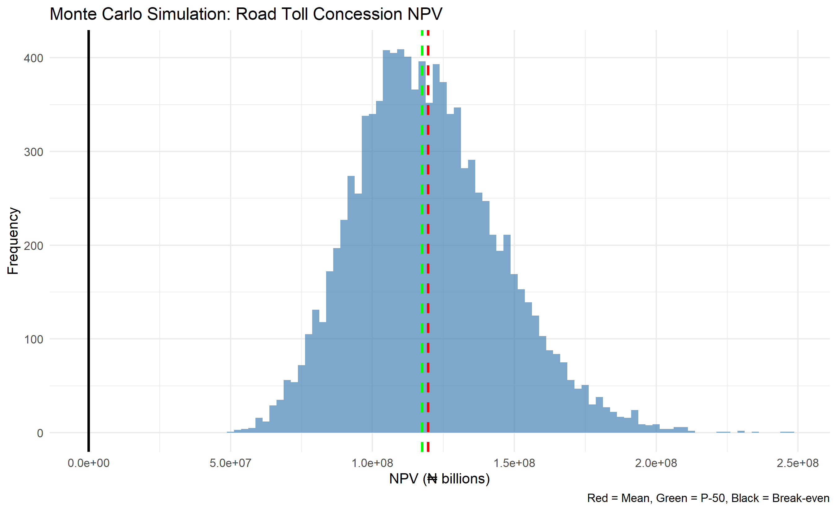
ggplot(simulations, aes(x = npv / 1000)) +
geom_histogram(bins = 100, fill = "steelblue", alpha = 0.7) +
geom_vline(aes(xintercept = npv_summary$mean_npv / 1000), color = "red", linetype = "dashed", linewidth = 1) +
geom_vline(aes(xintercept = npv_summary$p50 / 1000), color = "green", linetype = "dashed", linewidth = 1) +
geom_vline(aes(xintercept = 0), color = "black", linetype = "solid", linewidth = 1) +
labs(
title = "Monte Carlo Simulation: Road Toll Concession NPV",
x = "NPV (₦ billions)", y = "Frequency",
caption = "Red = Mean, Green = P-50, Black = Break-even"
) +
theme_minimal()
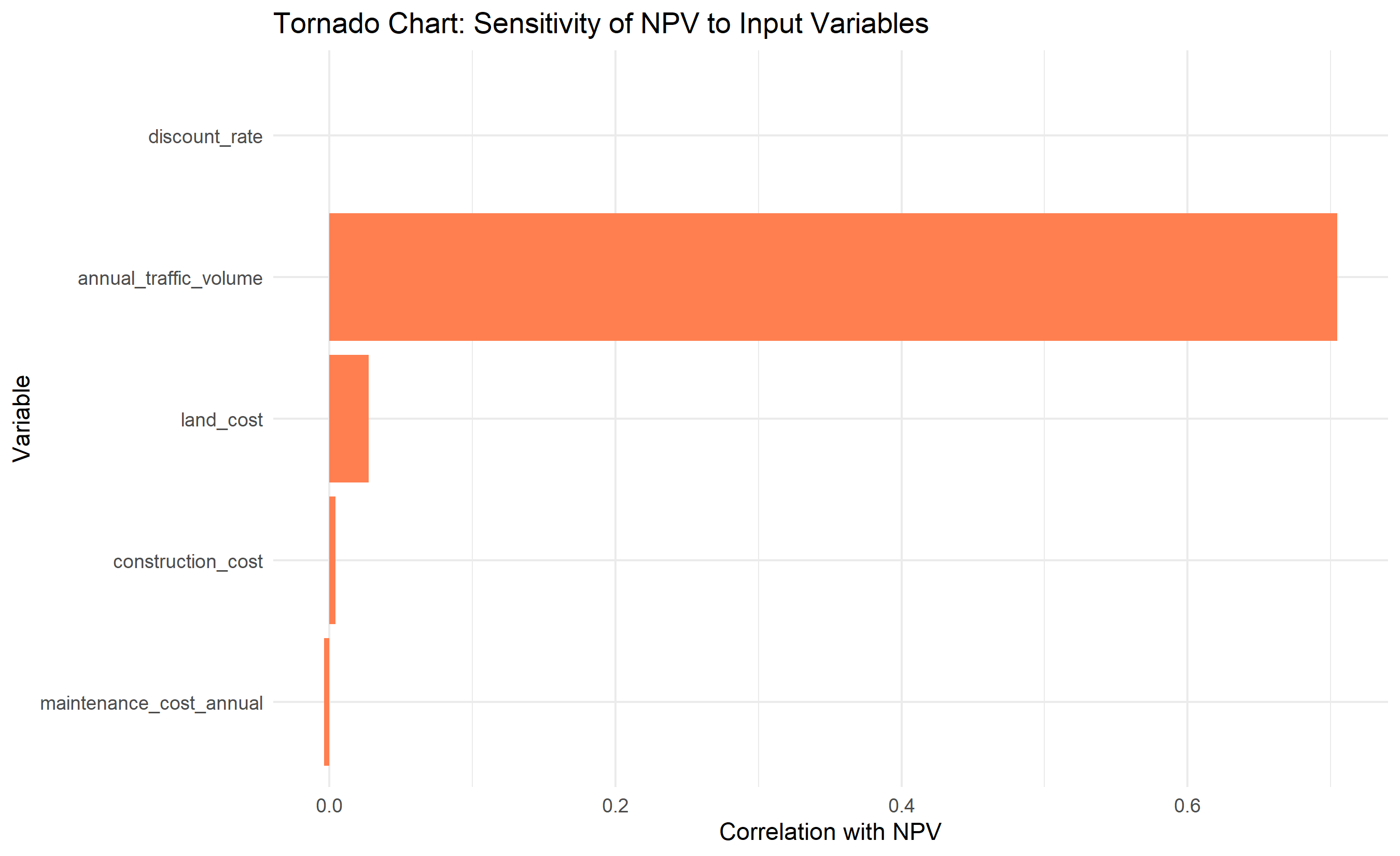
# Sensitivity analysis: tornado chart (correlation with NPV)
correlations <- list()
for (var in c("land_cost", "construction_cost", "annual_traffic_volume",
              "discount_rate", "maintenance_cost_annual")) {
  if (var %in% names(simulations)) {
    corr <- cor(simulations[[var]], simulations$npv)
    correlations[[var]] <- corr
  }
}

tornado_df <- tibble(
  variable = names(correlations),
  correlation = unlist(correlations)
) |>
  arrange(desc(abs(correlation)))

ggplot(tornado_df, aes(y = reorder(variable, abs(correlation)), x = correlation)) +
  geom_col(fill = "coral") +
  labs(
    title = "Tornado Chart: Sensitivity of NPV to Input Variables",
    y = "Variable", x = "Correlation with NPV"
  ) +
  theme_minimal()
```
## Python
```{python}
#| label: py-ch55-monte-carlo-workflow
import numpy as np
import pandas as pd
import matplotlib.pyplot as plt
np.random.seed(7463)
# Monte Carlo simulation
n_sim = 10000
simulations = pd.DataFrame({
'land_cost': np.random.lognormal(np.log(5000), 0.3, n_sim),
'construction_cost': np.random.normal(50000, 10000, n_sim),
'construction_months': np.random.normal(36, 6, n_sim),
'annual_traffic': np.random.normal(2000000, 300000, n_sim),
'toll_per_vehicle': 500,
'concession_years': 25,
'initial_fxrate': 800,
'discount_rate': 0.10,
'maintenance_annual': np.random.normal(5000, 1000, n_sim)
})
# FX rate
simulations['fxrate_end'] = simulations['initial_fxrate'] * np.exp(np.random.normal(-0.05, 0.15, n_sim))
# Delay cost
simulations['delay_cost'] = (simulations['construction_months'] / 12) * simulations['annual_traffic'] * 300 / 1000
# Revenue and costs
simulations['gross_revenue'] = ((simulations['annual_traffic'] * simulations['toll_per_vehicle'] *
simulations['concession_years'] - simulations['delay_cost']) *
simulations['fxrate_end'] / 100)
simulations['total_cost'] = (simulations['land_cost'] + simulations['construction_cost'] +
simulations['maintenance_annual'] * simulations['concession_years'])
simulations['npv'] = (simulations['gross_revenue'] - simulations['total_cost']) / (1 + simulations['discount_rate'])**5
# Summary
print("\n=== NPV Simulation Results ===")
print(f"Mean NPV (₦m): {simulations['npv'].mean():.0f}")
print(f"P-50 NPV (₦m): {simulations['npv'].median():.0f}")
print(f"P-80 NPV (₦m): {simulations['npv'].quantile(0.80):.0f}")
print(f"Probability of Positive NPV: {(simulations['npv'] > 0).mean() * 100:.1f}%")
# Visualization
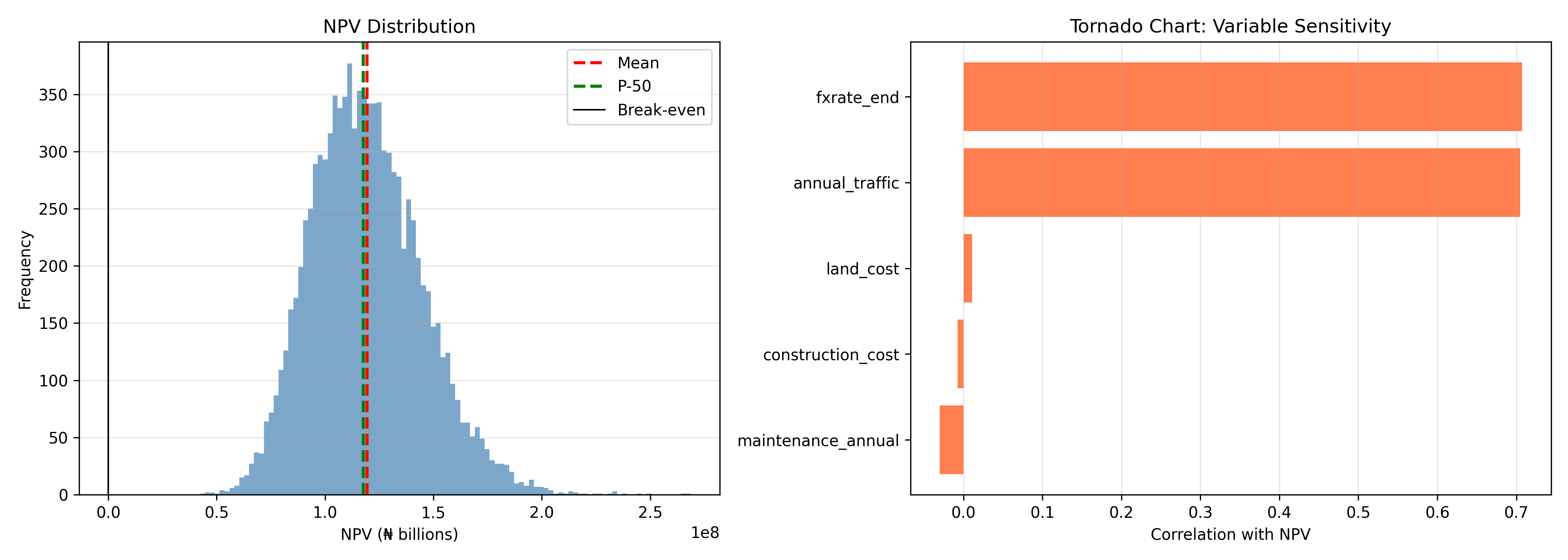
fig, (ax1, ax2) = plt.subplots(1, 2, figsize=(14, 5))
# Histogram
ax1.hist(simulations['npv'] / 1000, bins=100, color='steelblue', alpha=0.7)
ax1.axvline(simulations['npv'].mean() / 1000, color='red', linestyle='--', label='Mean', linewidth=2)
ax1.axvline(simulations['npv'].median() / 1000, color='green', linestyle='--', label='P-50', linewidth=2)
ax1.axvline(0, color='black', linestyle='-', label='Break-even', linewidth=1)
ax1.set_xlabel('NPV (₦ billions)')
ax1.set_ylabel('Frequency')
ax1.set_title('NPV Distribution')
ax1.legend()
ax1.grid(True, alpha=0.3, axis='y')
# Tornado (sensitivity)
correlations = {}
for col in ['land_cost', 'construction_cost', 'annual_traffic', 'maintenance_annual', 'fxrate_end']:
correlations[col] = np.corrcoef(simulations[col], simulations['npv'])[0, 1]
tornado_df = pd.DataFrame(list(correlations.items()), columns=['Variable', 'Correlation'])
tornado_df = tornado_df.sort_values('Correlation', ascending=True)
ax2.barh(tornado_df['Variable'], tornado_df['Correlation'], color='coral')
ax2.set_xlabel('Correlation with NPV')
ax2.set_title('Tornado Chart: Variable Sensitivity')
ax2.grid(True, alpha=0.3, axis='x')
plt.tight_layout()
plt.show()
```
:::
::: {.callout-caution icon="false"}
## 📝 Section 55.2 Review Questions
1. You are simulating project cost with three uncertain components: labor (Normal, μ=₦10m, σ=₦1m), materials (Lognormal), and equipment (Triangular, min=₦2m, mode=₦3m, max=₦5m). How would you justify your choice of each distribution?
2. In the simulation above, which input variable has the highest correlation with NPV? What does this tell you about where to focus risk mitigation efforts?
3. What is the relationship between N (number of simulations) and the width of the confidence interval for the estimated mean? If you want to halve the CI width, how much should you increase N?
4. A Nigerian pharmaceutical company is simulating the NPV of a drug development project. Costs are distributed Normal; time-to-market is skewed (could be very long if regulatory delays occur). Which distribution captures time-to-market better: Normal, Lognormal, or PERT?
5. In your simulation output, P-80 NPV is ₦2bn. Explain what this means to a non-technical stakeholder (e.g., the CFO).
:::
## Choosing the Right Distribution
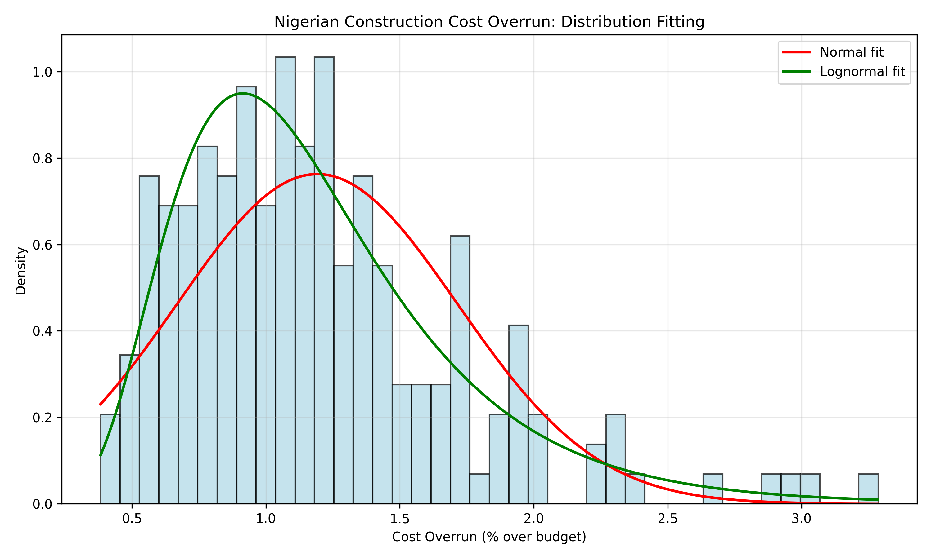
Different business variables exhibit different distributional patterns. Choosing the right distribution is crucial for realistic simulation:
- **Normal (Gaussian)**: Symmetric uncertainty around a point estimate. Use when: multiple independent causes of variation (labor hours, assembly time, symmetric cost overruns). Example: "Revenue is ₦100m ± 20m." Central limit theorem suggests normality for aggregate quantities.
- **Lognormal**: Right-skewed with a positive floor. Use when: the variable cannot go below zero and large upside exists (construction costs, supplier prices, equipment failures). Right-skew reflects typical project management: best case is on-time, but delays can cascade. For a cost variable, lognormal often better represents "typical cost is ₦50m, but could jump to ₦200m if complications arise."
- **Triangular**: Bounded by minimum, mode (most likely), and maximum. Use when: expert judgment provides three-point estimates and the distribution is approximately linear between them. Common in project management (PERT uses triangular as a base).
- **PERT (Program Evaluation and Review Technique)**: A smooth version of triangular with mean = (min + 4×mode + max) / 6. Use when: you want to weight the mode more heavily than triangular's linear interpolation, and you have project manager estimates.
- **Discrete/Scenario**: Use when: outcomes are categorical (three macroeconomic scenarios: growth, stable, downturn) or events have low probability (regulatory approval yes/no).
- **Poisson**: Use when: modeling count data with discrete jumps (customer arrivals, part failures, demand spikes).
::: {.panel-tabset}
## R
```{r}
#| label: ch55-distribution-fitting
library(tidyverse)
library(MASS)
set.seed(2938)
# Generate synthetic Nigerian construction cost overrun data (lognormal)
n <- 200
cost_overrun_pct <- rlnorm(n, meanlog = 0.15, sdlog = 0.45)
# Fit normal and lognormal distributions
fit_normal <- fitdistr(cost_overrun_pct, "normal")
fit_lognormal <- fitdistr(cost_overrun_pct, "lognormal")
# Compare AIC (lower is better)
aic_normal <- -2 * logLik(fit_normal) + 2 * 2
aic_lognormal <- -2 * logLik(fit_lognormal) + 2 * 2
cat("\nAIC - Normal:", round(as.numeric(aic_normal), 2), "\n")
cat("AIC - Lognormal:", round(as.numeric(aic_lognormal), 2), "\n")
cat("Better fit:", ifelse(aic_lognormal < aic_normal, "Lognormal", "Normal"), "\n")
# Plot histogram with fitted curves
df_plot <- tibble(x = cost_overrun_pct)
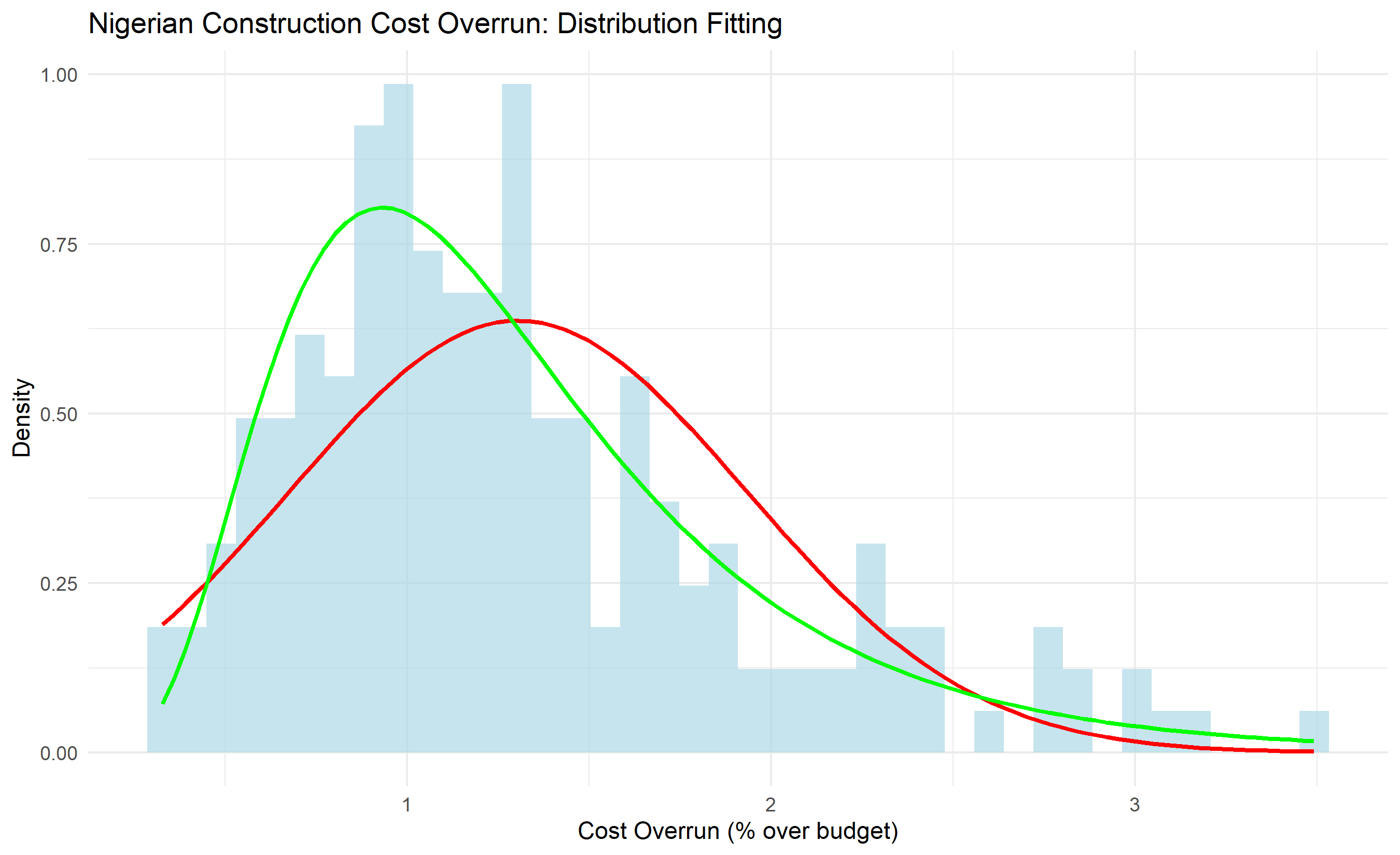
ggplot(df_plot, aes(x = x)) +
geom_histogram(aes(y = after_stat(density)), bins = 40, fill = "lightblue", alpha = 0.7) +
# Normal fit
stat_function(fun = dnorm, args = list(mean = coef(fit_normal)[1], sd = coef(fit_normal)[2]),
color = "red", size = 1, label = "Normal fit") +
# Lognormal fit
stat_function(fun = dlnorm, args = list(meanlog = coef(fit_lognormal)[1], sdlog = coef(fit_lognormal)[2]),
color = "green", size = 1, label = "Lognormal fit") +
labs(title = "Nigerian Construction Cost Overrun: Distribution Fitting",
x = "Cost Overrun (% over budget)", y = "Density") +
theme_minimal() +
theme(legend.position = "topright")
```
## Python
```{python}
#| label: py-ch55-distribution-fitting
import numpy as np
import pandas as pd
import matplotlib.pyplot as plt
from scipy import stats

np.random.seed(2938)

# Generate synthetic Nigerian construction cost overrun data (lognormal)
n = 200
cost_overrun_pct = np.random.lognormal(mean=0.15, sigma=0.45, size=n)

# Fit normal and lognormal distributions
params_normal = stats.norm.fit(cost_overrun_pct)
params_lognorm = stats.lognorm.fit(cost_overrun_pct, floc=0)

# Plot histogram with fitted curves
fig, ax = plt.subplots(figsize=(10, 6))

ax.hist(cost_overrun_pct, bins=40, density=True, alpha=0.7, color='lightblue', edgecolor='black')

# Normal fit
x_range = np.linspace(cost_overrun_pct.min(), cost_overrun_pct.max(), 200)
ax.plot(x_range, stats.norm.pdf(x_range, *params_normal), 'r-', linewidth=2, label='Normal fit')

# Lognormal fit
ax.plot(x_range, stats.lognorm.pdf(x_range, *params_lognorm), 'g-', linewidth=2, label='Lognormal fit')

ax.set_xlabel('Cost Overrun (% over budget)')
ax.set_ylabel('Density')
ax.set_title('Nigerian Construction Cost Overrun: Distribution Fitting')
ax.legend()
ax.grid(True, alpha=0.3)
plt.tight_layout()
plt.show()
# AIC comparison
aic_normal = 2*2 - 2*np.sum(stats.norm.logpdf(cost_overrun_pct, *params_normal))
aic_lognorm = 2*2 - 2*np.sum(stats.lognorm.logpdf(cost_overrun_pct, *params_lognorm))
print(f"AIC - Normal: {aic_normal:.2f}")
print(f"AIC - Lognormal: {aic_lognorm:.2f}")
print(f"Better fit: {'Lognormal' if aic_lognorm < aic_normal else 'Normal'}")
```
:::
::: {.callout-caution icon="false"}
## 📝 Section 55.3 Review Questions
1. What is the key difference between Normal and Lognormal distributions? When would you use Triangular vs PERT?
2. A Nigerian airline is modeling passenger demand. The distribution is likely right-skewed (capacity constraint on upside, but downside can be severe). Which distribution is most appropriate: Normal, Lognormal, or Triangular? Why?
3. You fit two distributions to historical cost data. Normal has AIC = 850, Lognormal has AIC = 823. Which should you use in your simulation? What does AIC measure?
4. PERT formula: mean = (min + 4×mode + max) / 6. How does this differ from Triangular? When is the PERT weighting justified?
5. A project manager estimates: "Labor cost: minimum ₦10m, most likely ₦12m, maximum ₦16m." Should you use Triangular or Lognormal? What additional information would help decide?
:::
## Variance Reduction Techniques
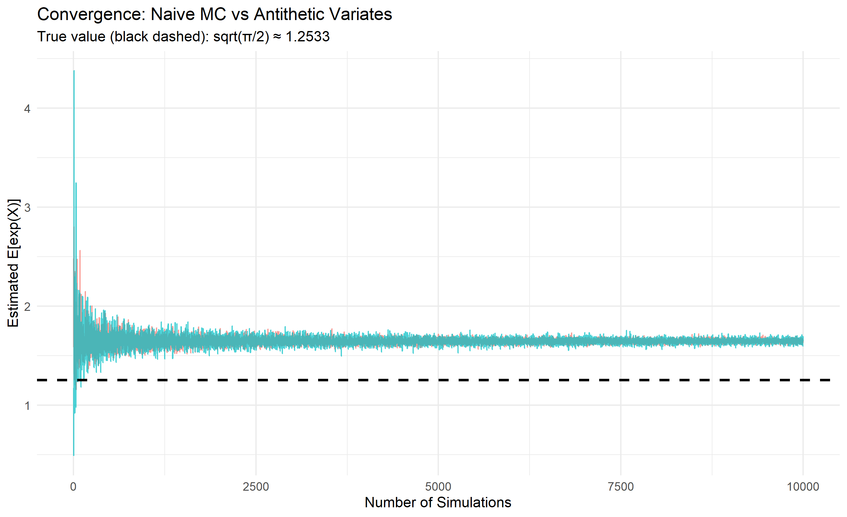
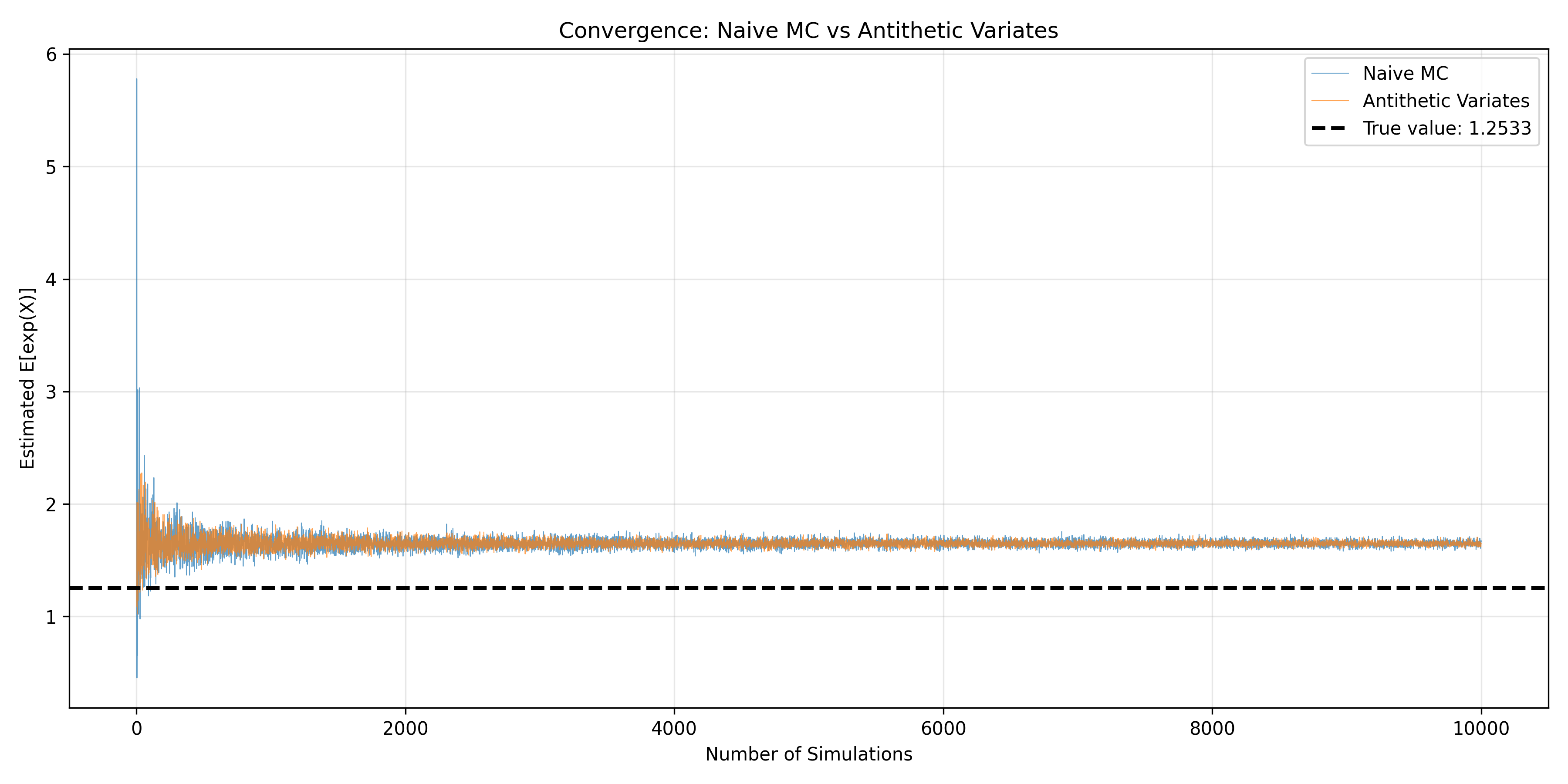
Standard Monte Carlo requires many samples for accurate estimates. **Variance reduction** techniques improve efficiency by reducing the variability of output estimates without increasing the number of samples.
**Antithetic Variates**: Generate pairs of random samples where one is the mirror image of the other. If $U \sim \text{Uniform}(0,1)$, sample both $U$ and $1-U$ and average their contributions. This negative correlation reduces variance. For a monotonic function $f$, if $Y = f(U)$ and $Y' = f(1-U)$, then $\text{Cov}(Y, Y') < 0$, so $\text{Var}[(Y + Y')/2] < \text{Var}[Y]$.
**Stratified Sampling**: Divide the range of each uncertain variable into equal-probability strata (e.g., deciles), then sample equal numbers from each stratum. This ensures representation of all quantiles, eliminating sampling luck.
**Latin Hypercube Sampling (LHS)**: For $N$ samples and $d$ uncertain dimensions, divide each dimension into $N$ intervals of equal probability. Sample once from each interval per dimension, but permute the order randomly across dimensions. This ensures good coverage in high-dimensional space more efficiently than random sampling.
::: {.panel-tabset}
## R
```{r}
#| label: ch55-variance-reduction
library(tidyverse)

set.seed(5174)

# Naive Monte Carlo vs Antithetic Variates
# Estimating E[exp(X)] where X ~ N(0, 1)

n_max <- 10000
naive_estimates <- numeric(n_max)
antithetic_estimates <- numeric(n_max)

for (n in 1:n_max) {
  # Naive MC: independent samples
  u_naive <- rnorm(n)
  naive_estimates[n] <- mean(exp(u_naive))

  # Antithetic: pairs of U and -U
  u_pairs <- rnorm(n/2)
  antithetic_estimates[n] <- mean(exp(c(u_pairs, -u_pairs)))
}

# Plot convergence
convergence_df <- tibble(
  n = 1:n_max,
  naive = naive_estimates,
  antithetic = antithetic_estimates
) |>
  pivot_longer(cols = -n, names_to = "method", values_to = "estimate")

ggplot(convergence_df, aes(x = n, y = estimate, color = method)) +
  geom_line(alpha = 0.7, linewidth = 0.5) +
  geom_hline(aes(yintercept = sqrt(pi / 2)), linetype = "dashed", color = "black", linewidth = 1) +
  labs(
    title = "Convergence: Naive MC vs Antithetic Variates",
    x = "Number of Simulations", y = "Estimated E[exp(X)]",
    subtitle = "True value (black dashed): sqrt(π/2) ≈ 1.2533"
  ) +
  theme_minimal() +
  theme(legend.position = "bottomright")
# Variance reduction at N=1000
variance_naive <- var(naive_estimates[1:1000])
variance_antithetic <- var(antithetic_estimates[1:1000])
reduction_factor <- variance_naive / variance_antithetic
cat("\nVariance at N=1000:\n")
cat("Naive MC:", round(variance_naive, 6), "\n")
cat("Antithetic:", round(variance_antithetic, 6), "\n")
cat("Variance reduction factor:", round(reduction_factor, 2), "\n")
```
## Python
```{python}
#| label: py-ch55-variance-reduction
import numpy as np
import pandas as pd
import matplotlib.pyplot as plt

np.random.seed(5174)

# Naive Monte Carlo vs Antithetic Variates
# Estimating E[exp(X)] where X ~ N(0, 1)

n_max = 10000
naive_estimates = np.zeros(n_max)
antithetic_estimates = np.zeros(n_max)

for n in range(1, n_max + 1):
    # Naive MC: independent samples
    u_naive = np.random.normal(0, 1, n)
    naive_estimates[n-1] = np.mean(np.exp(u_naive))

    # Antithetic: pairs of U and -U
    n_half = n // 2
    u_pairs = np.random.normal(0, 1, n_half)
    antithetic_estimates[n-1] = np.mean(np.exp(np.concatenate([u_pairs, -u_pairs])))

# Plot convergence
fig, ax = plt.subplots(figsize=(12, 6))

ax.plot(range(1, n_max + 1), naive_estimates, label='Naive MC', alpha=0.7, linewidth=0.5)
ax.plot(range(1, n_max + 1), antithetic_estimates, label='Antithetic Variates', alpha=0.7, linewidth=0.5)
ax.axhline(y=np.sqrt(np.pi / 2), color='black', linestyle='--', linewidth=2, label=f'True value: {np.sqrt(np.pi/2):.4f}')

ax.set_xlabel('Number of Simulations')
ax.set_ylabel('Estimated E[exp(X)]')
ax.set_title('Convergence: Naive MC vs Antithetic Variates')
ax.legend()
ax.grid(True, alpha=0.3)
plt.tight_layout()
plt.show()
# Variance reduction at N=1000
var_naive = np.var(naive_estimates[:1000])
var_antithetic = np.var(antithetic_estimates[:1000])
reduction_factor = var_naive / var_antithetic
print(f"\nVariance at N=1000:")
print(f"Naive MC: {var_naive:.6f}")
print(f"Antithetic: {var_antithetic:.6f}")
print(f"Variance reduction factor: {reduction_factor:.2f}x")
```
:::
::: {.callout-caution icon="false"}
## 📝 Section 55.4 Review Questions
1. What is antithetic variates? How does it reduce variance without increasing sample size?
2. Explain Latin Hypercube Sampling (LHS). When is it more efficient than random sampling?
3. You estimate a portfolio's Value at Risk with 10,000 naive MC samples. Your confidence interval for the VaR-95% is ± ₦50m. You switch to LHS and reduce variance by 4×. What is your new CI width?
4. Stratified sampling divides each variable into quantile bins. How does this prevent "bad luck" in sampling?
5. A Monte Carlo project simulation shows P(NPV > 0) = 48% with N=10,000. This is borderline; should you invest? What would antithetic variates or LHS add to your confidence in this result?
:::
## Business Applications: Project Risk and Portfolio VaR
### Project NPV Simulation
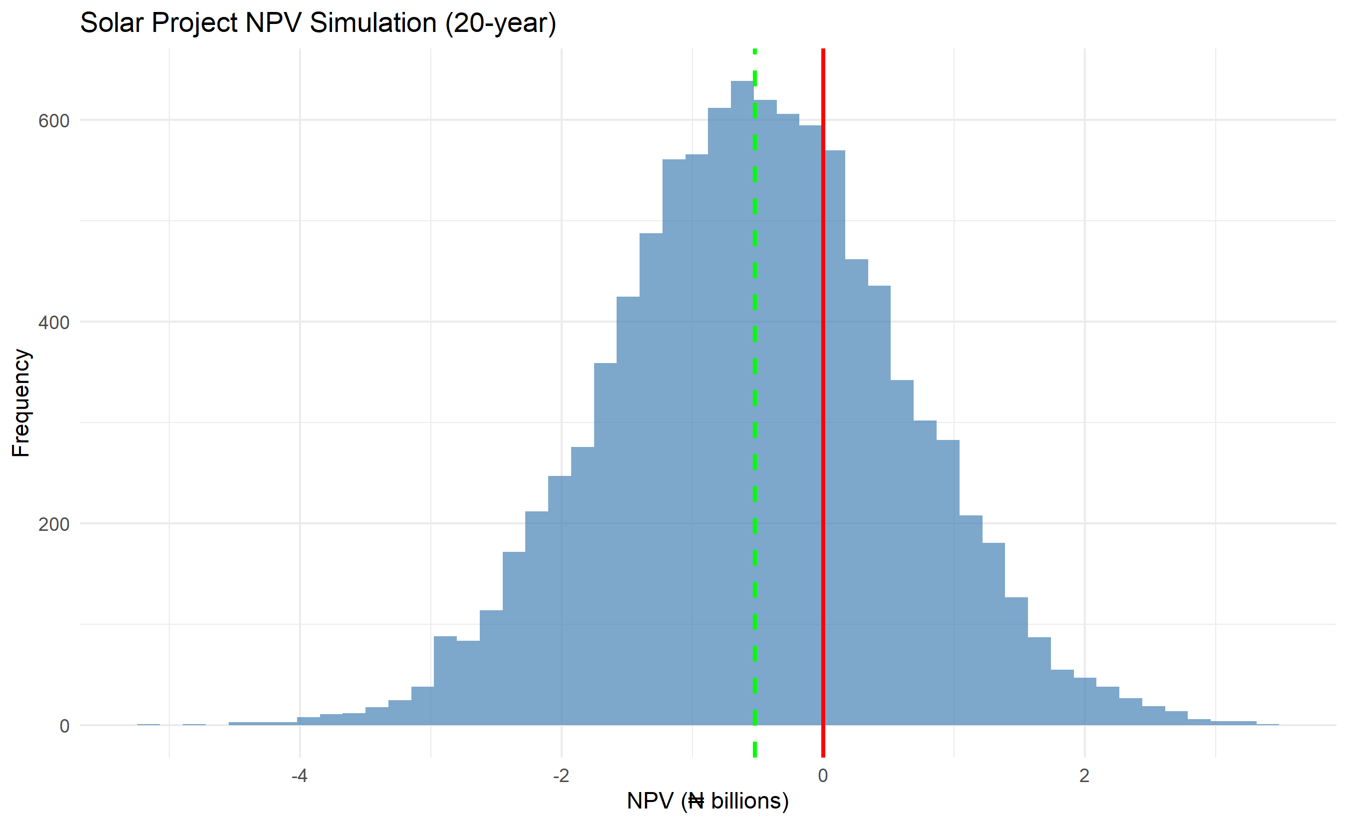
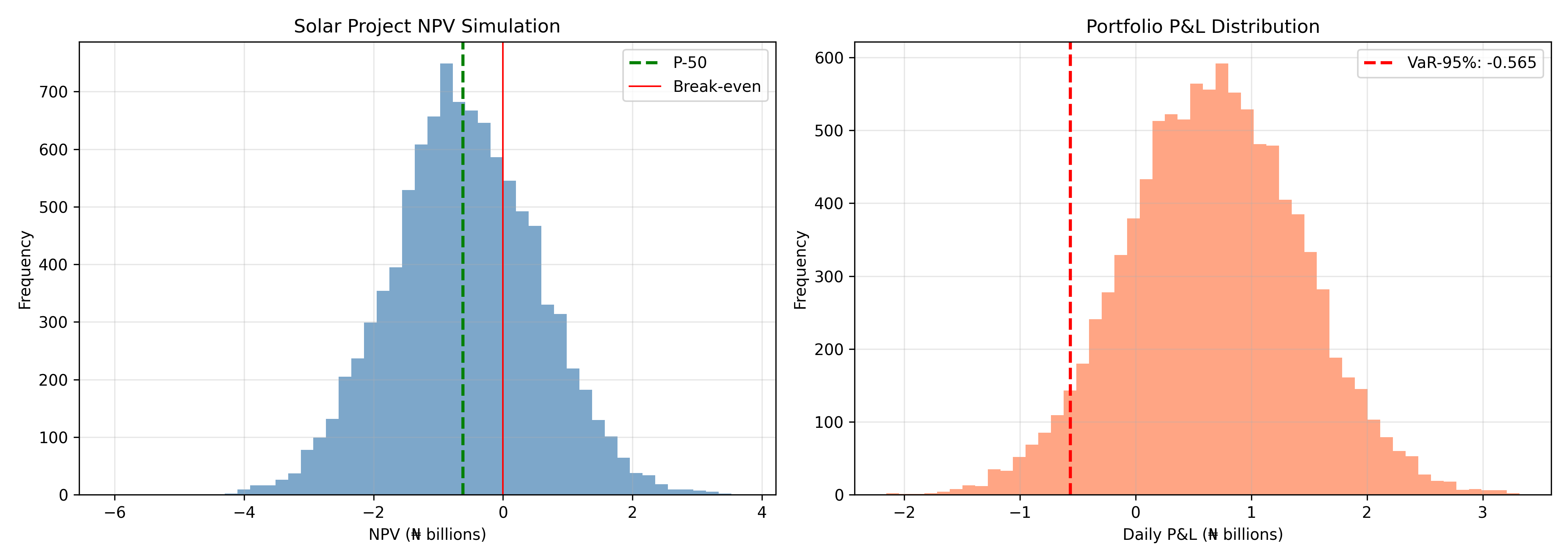
Construction and infrastructure projects face correlated uncertainties. A solar power plant in Lagos must estimate: revenue (demand × tariff, both uncertain), CAPEX (procurement + execution risk), OPEX (labor, utilities, maintenance), and discount rate (cost of capital depends on inflation expectations).
Simulating 10,000 project scenarios produces not just expected NPV, but P-10, P-50, P-90 percentiles—allowing the CFO to allocate budget reserves and the board to assess downside risk.
### Portfolio Value at Risk (VaR)
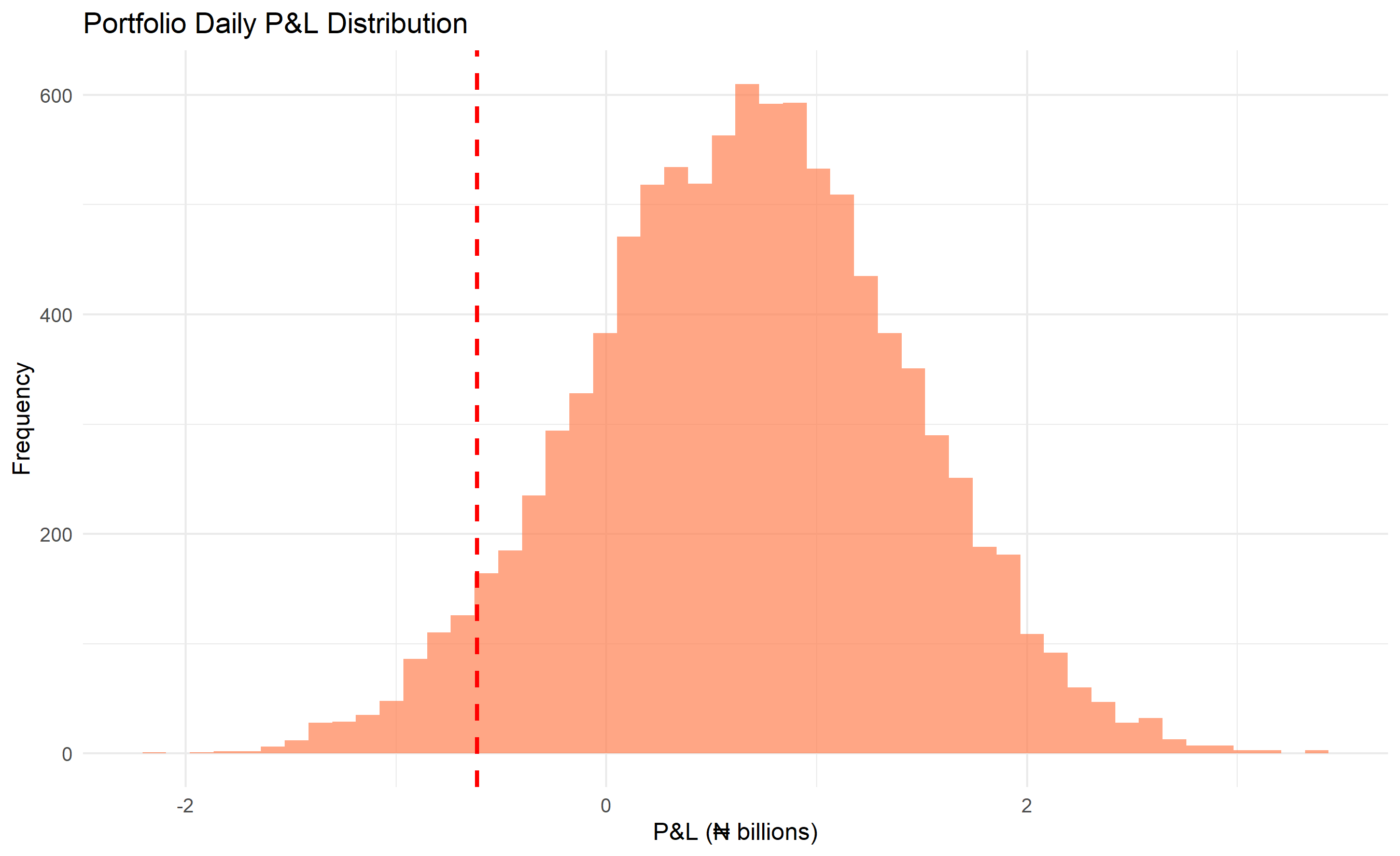
A bank's portfolio contains loans, equities, and FX positions. VaR-95% answers: "In 95% of scenarios, what is the maximum daily loss?" Compute via simulation:
1. Model return distributions for each asset (correlated)
2. Simulate 10,000+ market scenarios one day forward
3. Compute portfolio P&L for each scenario
4. Extract the 5th percentile loss
::: {.panel-tabset}
## R
```{r}
#| label: ch55-npv-simulation
library(tidyverse)
library(MASS)
set.seed(8627)
# Helper function for triangular distribution (not in base R)
rtriangle <- function(n, a, b, c) {
u <- runif(n)
fc <- (c - a) / (b - a)
idx_lower <- u <= fc
result <- numeric(n)
result[idx_lower] <- a + sqrt(u[idx_lower] * (b - a) * (c - a))
result[!idx_lower] <- b - sqrt((1 - u[!idx_lower]) * (b - a) * (b - c))
result
}
# NPV Simulation: Nigerian Solar Power Plant (20-year project)
n_sim <- 10000
# Define correlation structure
corr_matrix <- matrix(c(
1.0, -0.5, 0.3,
-0.5, 1.0, 0.2,
0.3, 0.2, 1.0
), nrow = 3)
# Correlated uncertain inputs: log revenue, OPEX factor, FX volatility
mean_vector <- c(0, 0, 0)
correlated_inputs <- mvrnorm(n = n_sim, mu = mean_vector, Sigma = corr_matrix)
project_sim <- tibble(
# Revenue: N(₦500m/yr, ₦80m/yr) [tariff + demand uncertainty]
annual_revenue = rnorm(n_sim, 500, 80) + 100 * correlated_inputs[, 1],
# CAPEX: Lognormal(₦3bn, ₦400m)
capex = rlnorm(n_sim, log(3000), 0.15),
# OPEX: N(₦150m/yr, ₦20m/yr)
annual_opex = rnorm(n_sim, 150, 20) + 30 * correlated_inputs[, 2],
# Discount rate: Triangular(10%, 12%, 18%)
discount_rate = rtriangle(n_sim, 0.10, 0.12, 0.18),
# Project life
project_years = 20
) |>
mutate(
# NPV calculation (simplified: uniform annual cash flows)
annual_cf = annual_revenue - annual_opex,
pv_annuity = annual_cf * (1 - (1 + discount_rate)^(-project_years)) / discount_rate,
npv = pv_annuity - capex
)
# Summary
npv_quantiles <- quantile(project_sim$npv, probs = c(0.10, 0.25, 0.50, 0.75, 0.90))
cat("\n=== Solar Project NPV (₦ millions) ===\n")
cat("P-10 NPV:", round(npv_quantiles["10%"], 0), "\n")
cat("P-50 NPV:", round(npv_quantiles["50%"], 0), "\n")
cat("P-90 NPV:", round(npv_quantiles["90%"], 0), "\n")
cat("P(NPV > 0):", round(mean(project_sim$npv > 0) * 100, 1), "%\n")
# Visualization
ggplot(project_sim, aes(x = npv / 1000)) +
geom_histogram(bins = 50, fill = "steelblue", alpha = 0.7) +
geom_vline(aes(xintercept = npv_quantiles["50%"] / 1000), color = "green", linewidth = 1, linetype = "dashed") +
geom_vline(aes(xintercept = 0), color = "red", linewidth = 1, linetype = "solid") +
labs(title = "Solar Project NPV Simulation (20-year)",
x = "NPV (₦ billions)", y = "Frequency") +
theme_minimal()
# Portfolio VaR simulation (3-asset portfolio)
set.seed(3859)
n_sim <- 10000
# Asset returns (correlated): equities, bonds, cash
returns_corr <- matrix(c(
1.0, -0.2, 0.1,
-0.2, 1.0, 0.5,
0.1, 0.5, 1.0
), nrow = 3)
mean_returns <- c(0.10, 0.04, 0.02)
cov_matrix <- diag(c(0.15, 0.08, 0.02)) %*% returns_corr %*% diag(c(0.15, 0.08, 0.02))
asset_returns <- mvrnorm(n = n_sim, mu = mean_returns, Sigma = cov_matrix)
# Portfolio weights
w_equity <- 0.50
w_bond <- 0.35
w_cash <- 0.15
portfolio_returns <- w_equity * asset_returns[, 1] +
w_bond * asset_returns[, 2] +
w_cash * asset_returns[, 3]
# Portfolio value in ₦ billions
portfolio_value <- 10 # ₦10bn
portfolio_pnl <- portfolio_returns * portfolio_value
var_95 <- quantile(portfolio_pnl, 0.05)
cvar_95 <- mean(portfolio_pnl[portfolio_pnl <= var_95])
cat("\n=== Portfolio VaR (₦ billions) ===\n")
cat("VaR-95%:", round(var_95, 3), "\n")
cat("CVaR-95% (Expected Shortfall):", round(cvar_95, 3), "\n")
# Plot
ggplot(tibble(pnl = portfolio_pnl), aes(x = pnl)) +
geom_histogram(bins = 50, fill = "coral", alpha = 0.7) +
geom_vline(aes(xintercept = var_95), color = "red", linewidth = 1, linetype = "dashed",
label = paste("VaR-95%:", round(var_95, 3))) +
labs(title = "Portfolio Daily P&L Distribution",
x = "P&L (₦ billions)", y = "Frequency") +
theme_minimal()
```
## Python
```{python}
#| label: py-ch55-npv-var-simulation
import numpy as np
import pandas as pd
import matplotlib.pyplot as plt
from scipy.stats import multivariate_normal
np.random.seed(8627)
# NPV Simulation: Nigerian Solar Power Plant
n_sim = 10000
# Correlation matrix for 3 inputs
corr_matrix = np.array([
[1.0, -0.5, 0.3],
[-0.5, 1.0, 0.2],
[0.3, 0.2, 1.0]
])
# Covariance from correlation
cov_matrix = corr_matrix
correlated_inputs = np.random.multivariate_normal(np.zeros(3), corr_matrix, n_sim)
project_sim = pd.DataFrame({
'annual_revenue': np.random.normal(500, 80, n_sim) + 100 * correlated_inputs[:, 0],
'capex': np.random.lognormal(np.log(3000), 0.15, n_sim),
'annual_opex': np.random.normal(150, 20, n_sim) + 30 * correlated_inputs[:, 1],
})
# Discount rate: triangular(10%, 12%, 18%)
project_sim['discount_rate'] = np.random.triangular(0.10, 0.12, 0.18, n_sim)
project_sim['project_years'] = 20
# NPV calculation
project_sim['annual_cf'] = project_sim['annual_revenue'] - project_sim['annual_opex']
project_sim['pv_annuity'] = (project_sim['annual_cf'] *
(1 - (1 + project_sim['discount_rate'])**(-project_sim['project_years'])) /
project_sim['discount_rate'])
project_sim['npv'] = project_sim['pv_annuity'] - project_sim['capex']
# Summary
npv_stats = project_sim['npv'].describe()
print("\n=== Solar Project NPV (₦ millions) ===")
print(f"P-10 NPV: {project_sim['npv'].quantile(0.10):.0f}")
print(f"P-50 NPV: {project_sim['npv'].quantile(0.50):.0f}")
print(f"P-90 NPV: {project_sim['npv'].quantile(0.90):.0f}")
print(f"P(NPV > 0): {(project_sim['npv'] > 0).mean() * 100:.1f}%")
# Portfolio VaR (3 assets)
np.random.seed(3859)
n_sim = 10000
mean_returns = np.array([0.10, 0.04, 0.02])
cov_asset = np.diag([0.15, 0.08, 0.02]) @ np.array([
[1.0, -0.2, 0.1],
[-0.2, 1.0, 0.5],
[0.1, 0.5, 1.0]
]) @ np.diag([0.15, 0.08, 0.02])
asset_returns = np.random.multivariate_normal(mean_returns, cov_asset, n_sim)
# Portfolio
weights = np.array([0.50, 0.35, 0.15])
portfolio_returns = asset_returns @ weights
portfolio_value = 10 # ₦10bn
portfolio_pnl = portfolio_returns * portfolio_value
var_95 = np.percentile(portfolio_pnl, 5)
cvar_95 = portfolio_pnl[portfolio_pnl <= var_95].mean()
print(f"\n=== Portfolio VaR (₦ billions) ===")
print(f"VaR-95%: {var_95:.3f}")
print(f"CVaR-95%: {cvar_95:.3f}")
# Visualizations
fig, (ax1, ax2) = plt.subplots(1, 2, figsize=(14, 5))
# NPV histogram
ax1.hist(project_sim['npv'] / 1000, bins=50, color='steelblue', alpha=0.7)
ax1.axvline(project_sim['npv'].median() / 1000, color='green', linestyle='--', linewidth=2, label='P-50')
ax1.axvline(0, color='red', linestyle='-', linewidth=1, label='Break-even')
ax1.set_xlabel('NPV (₦ billions)')
ax1.set_ylabel('Frequency')
ax1.set_title('Solar Project NPV Simulation')
ax1.legend()
ax1.grid(True, alpha=0.3)
# Portfolio VaR
ax2.hist(portfolio_pnl, bins=50, color='coral', alpha=0.7)
ax2.axvline(var_95, color='red', linestyle='--', linewidth=2, label=f'VaR-95%: {var_95:.3f}')
ax2.set_xlabel('Daily P&L (₦ billions)')
ax2.set_ylabel('Frequency')
ax2.set_title('Portfolio P&L Distribution')
ax2.legend()
ax2.grid(True, alpha=0.3)
plt.tight_layout()
plt.show()
```
:::
::: {.callout-caution icon="false"}
## 📝 Section 55.5 Review Questions
1. A project has P(NPV > 0) = 72%. Should the company invest? What additional analysis would you request?
2. You simulate a project's NPV: P-50 = ₦5bn, P-90 = ₦2bn. How would you explain "P-90" to a non-technical CFO?
3. In portfolio VaR, why is CVaR (Expected Shortfall) often considered more useful than VaR for risk management?
4. The solar project simulation assumes uniform annual cash flows. How would you handle a project with ramp-up years (lower cash flows initially)?
5. A portfolio has VaR-95% = ₦500m. Does this mean 5% of days you lose ₦500m or more? Explain the precise interpretation.
:::
## Monte Carlo for Option Pricing
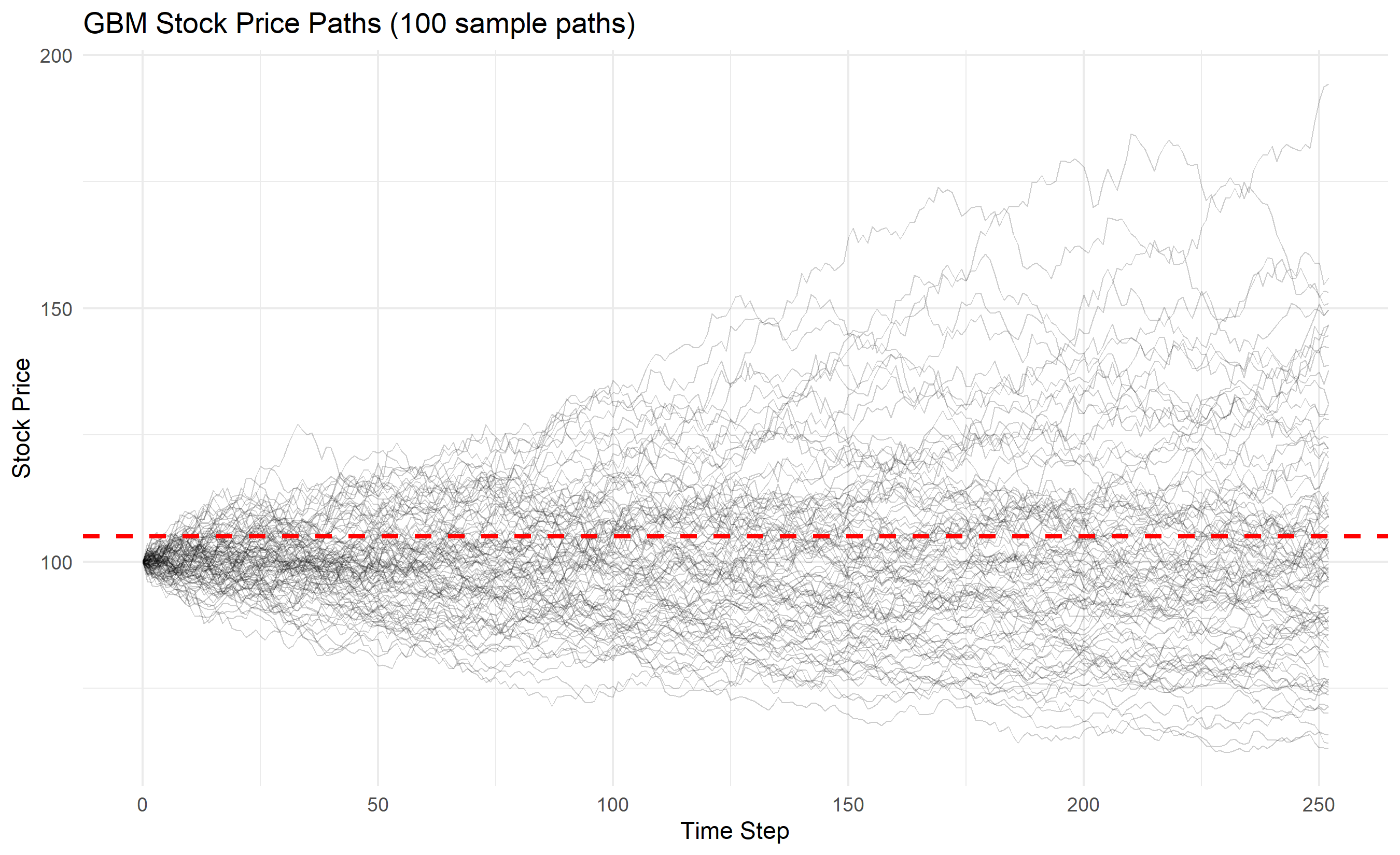
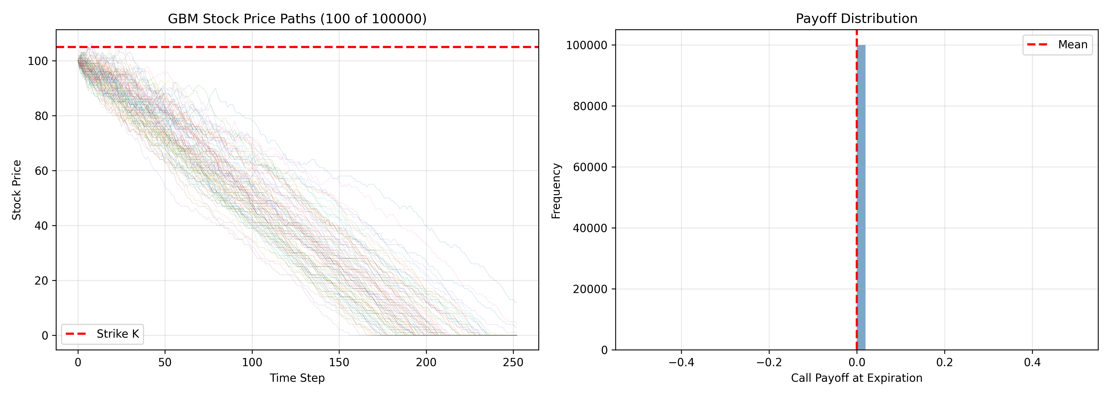
The Black-Scholes formula prices European vanilla options under restrictive assumptions (constant volatility, no transaction costs, European exercise). For American options (early exercise) or exotic payoffs (barriers, lookbacks, path-dependent), no closed form exists. Monte Carlo simulation is the standard approach:
1. Simulate stock price paths via geometric Brownian motion (GBM): $dS = \mu S dt + \sigma S dW$
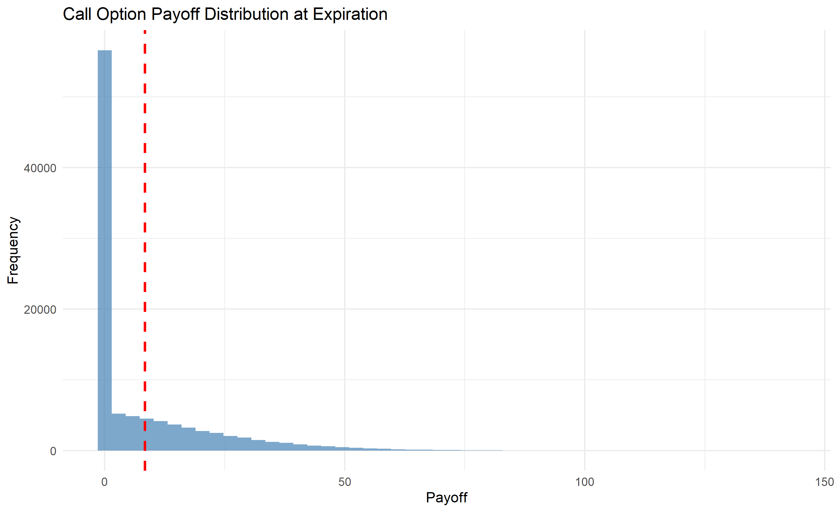
2. At each path's expiration, compute payoff (e.g., $\max(S_T - K, 0)$ for a call)
3. Discount payoffs back to present, take the average
::: {.panel-tabset}
## R
```{r}
#| label: ch55-option-pricing
library(tidyverse)
# European Call Option: GBM Simulation vs Black-Scholes
# Parameters
S0 <- 100 # Initial stock price
K <- 105 # Strike price
r <- 0.05 # Risk-free rate
sigma <- 0.20 # Volatility
T <- 1.0 # Time to expiration (1 year)
n_paths <- 100000
n_steps <- 252 # Daily steps
# Black-Scholes closed-form solution
d1 <- (log(S0 / K) + (r + 0.5 * sigma^2) * T) / (sigma * sqrt(T))
d2 <- d1 - sigma * sqrt(T)
bs_price <- S0 * pnorm(d1) - K * exp(-r * T) * pnorm(d2)
# Monte Carlo simulation
set.seed(6241)
dt <- T / n_steps
paths <- matrix(S0, nrow = n_paths, ncol = n_steps + 1)
for (step in 1:n_steps) {
Z <- rnorm(n_paths)
paths[, step + 1] <- paths[, step] * exp((r - 0.5 * sigma^2) * dt + sigma * sqrt(dt) * Z)
}
# Payoff: call option
payoffs <- pmax(paths[, n_steps + 1] - K, 0)
mc_price <- mean(payoffs) * exp(-r * T)
mc_se <- sd(payoffs) * exp(-r * T) / sqrt(n_paths)
cat("\n=== European Call Option Pricing ===\n")
cat("Parameters: S0 =", S0, ", K =", K, ", r =", r, ", σ =", sigma, ", T =", T, "\n")
cat("Black-Scholes Price:", round(bs_price, 4), "\n")
cat("Monte Carlo Price:", round(mc_price, 4), "±", round(1.96 * mc_se, 4), "\n")
cat("Difference:", round(abs(bs_price - mc_price), 4), "\n")
# Visualization: sample paths and payoff distribution
sample_paths_df <- as_tibble(t(paths[1:100, ])) |>
mutate(step = 0:n_steps) |>
pivot_longer(cols = -step, names_to = "path", values_to = "price")
ggplot(sample_paths_df, aes(x = step, y = price, group = path)) +
geom_line(alpha = 0.2, linewidth = 0.3) +
geom_hline(aes(yintercept = K), color = "red", linetype = "dashed", linewidth = 1, label = "Strike K") +
labs(title = "GBM Stock Price Paths (100 sample paths)",
x = "Time Step", y = "Stock Price") +
theme_minimal() +
theme(legend.position = "topright")
# Payoff distribution
payoff_df <- tibble(payoff = payoffs)
ggplot(payoff_df, aes(x = payoff)) +
  geom_histogram(bins = 50, fill = "steelblue", alpha = 0.7) +
  geom_vline(aes(xintercept = mean(payoff)), color = "red", linewidth = 1, linetype = "dashed") +
  labs(title = "Call Option Payoff Distribution at Expiration",
       x = "Payoff", y = "Frequency") +
  theme_minimal()
```
## Python
```{python}
#| label: py-ch55-option-pricing
import numpy as np
import pandas as pd
import matplotlib.pyplot as plt
from scipy.stats import norm
# Parameters
S0 = 100 # Initial stock price
K = 105 # Strike price
r = 0.05 # Risk-free rate
sigma = 0.20 # Volatility
T = 1.0 # Time to expiration
n_paths = 100000
n_steps = 252 # Daily steps
# Black-Scholes
d1 = (np.log(S0 / K) + (r + 0.5 * sigma**2) * T) / (sigma * np.sqrt(T))
d2 = d1 - sigma * np.sqrt(T)
bs_price = S0 * norm.cdf(d1) - K * np.exp(-r * T) * norm.cdf(d2)
# Monte Carlo
np.random.seed(6241)
dt = T / n_steps
paths = np.full((n_paths, n_steps + 1), S0)
for step in range(n_steps):
Z = np.random.normal(0, 1, n_paths)
paths[:, step + 1] = paths[:, step] * np.exp((r - 0.5 * sigma**2) * dt + sigma * np.sqrt(dt) * Z)
# Payoff
payoffs = np.maximum(paths[:, -1] - K, 0)
mc_price = np.mean(payoffs) * np.exp(-r * T)
mc_se = np.std(payoffs) * np.exp(-r * T) / np.sqrt(n_paths)
print(f"\n=== European Call Option Pricing ===")
print(f"S0={S0}, K={K}, r={r}, σ={sigma}, T={T}")
print(f"Black-Scholes Price: {bs_price:.4f}")
print(f"Monte Carlo Price: {mc_price:.4f} ± {1.96 * mc_se:.4f}")
print(f"Difference: {abs(bs_price - mc_price):.4f}")
# Visualizations
fig, (ax1, ax2) = plt.subplots(1, 2, figsize=(14, 5))
# Sample paths
for i in range(100):
ax1.plot(paths[i, :], alpha=0.2, linewidth=0.5)
ax1.axhline(K, color='red', linestyle='--', linewidth=2, label='Strike K')
ax1.set_xlabel('Time Step')
ax1.set_ylabel('Stock Price')
ax1.set_title(f'GBM Stock Price Paths (100 of {n_paths})')
ax1.legend()
ax1.grid(True, alpha=0.3)
# Payoff distribution
ax2.hist(payoffs, bins=50, color='steelblue', alpha=0.7)
ax2.axvline(np.mean(payoffs), color='red', linestyle='--', linewidth=2, label='Mean')
ax2.set_xlabel('Call Payoff at Expiration')
ax2.set_ylabel('Frequency')
ax2.set_title('Payoff Distribution')
ax2.legend()
ax2.grid(True, alpha=0.3)
plt.tight_layout()
plt.show()
```
:::
::: {.callout-caution icon="false"}
## 📝 Section 55.6 Review Questions
1. What are three main advantages of Monte Carlo for option pricing over Black-Scholes closed-form formula?
2. A European call option has S0=₦1000, K=₦1050, T=6 months. Simulate 10,000 paths. How does the MC price compare to Black-Scholes?
3. Why is geometric Brownian motion (GBM) appropriate for stock prices? What are its limitations?
4. How would you modify the code to price an American option (which allows early exercise)?
5. In the payoff distribution, why do many paths result in zero payoff? What does this imply for option value?
:::
## Case Study: Capital Project Risk Analysis for Nigerian Infrastructure
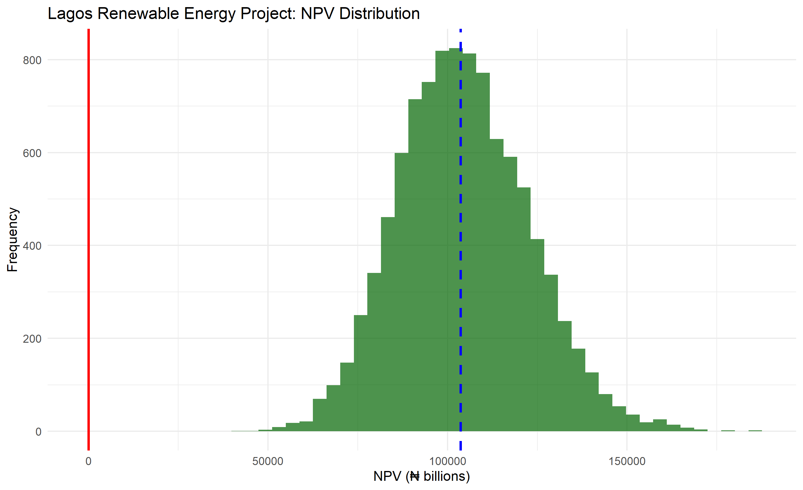
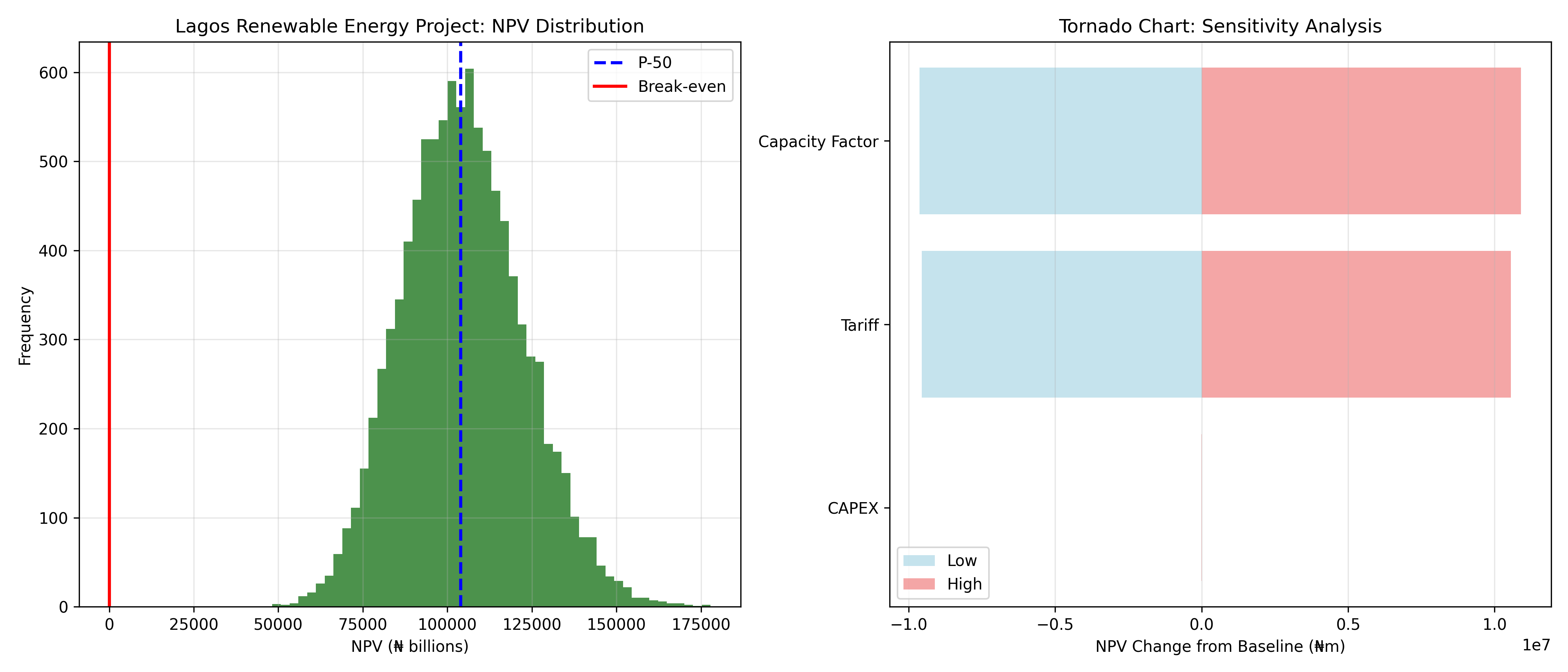
A ₦100 billion renewable energy plant (solar + battery storage) in Lagos faces multiple correlated uncertainties: construction cost overruns (common in Nigeria due to supply chain volatility and FX), electricity tariff negotiations with utilities, FX rate (USD costs, Naira cash flows), technical performance (capacity factor uncertainty), and delay risk (permitting, land acquisition).
This case demonstrates integrating:
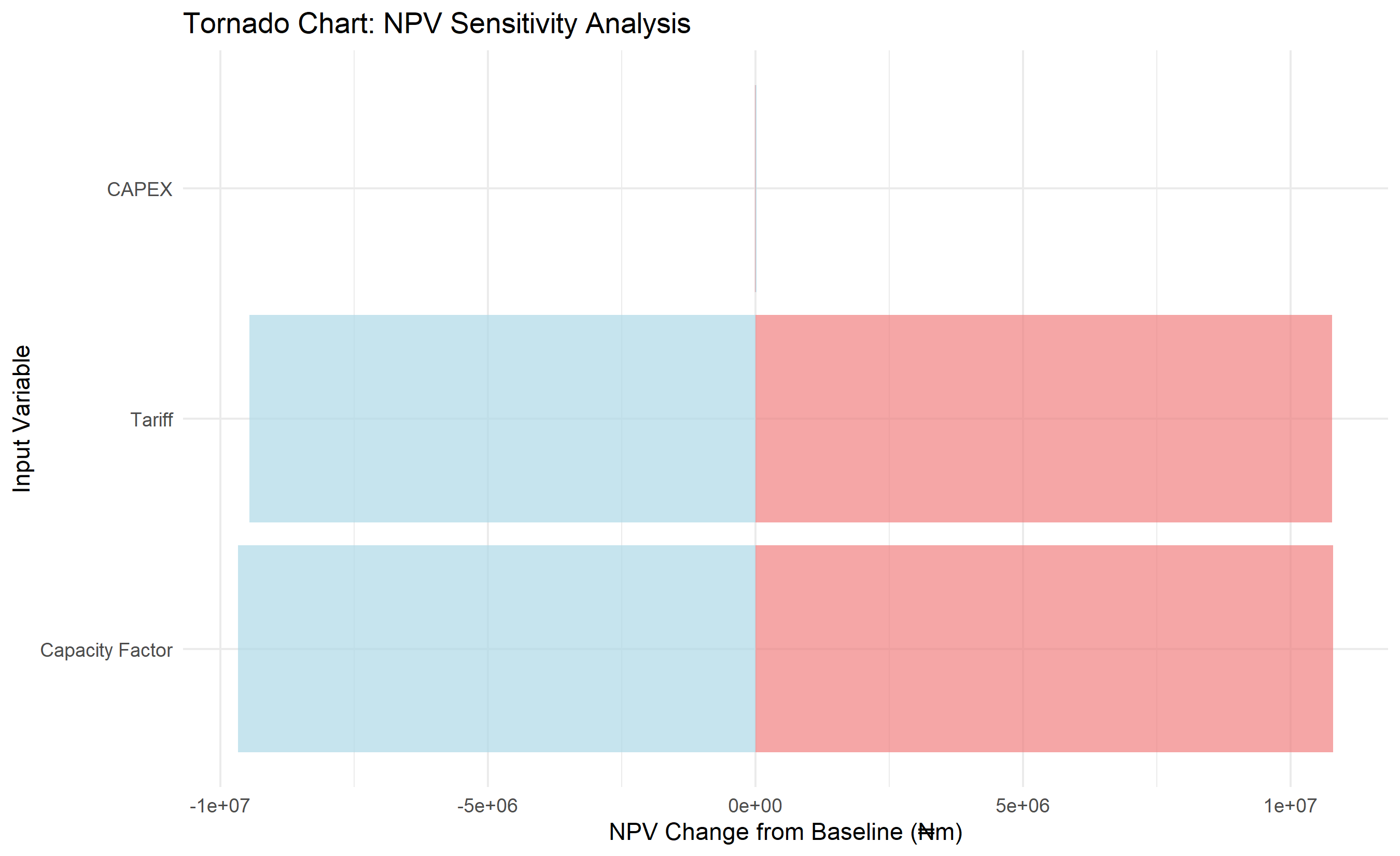
- Correlated input sampling (mvrnorm, multivariate_normal)
- Tornado chart for sensitivity
- Probability contours for decision support
- Risk-adjusted recommendation
::: {.panel-tabset}
## R
```{r}
#| label: ch55-case-study-infrastructure
library(tidyverse)
library(MASS)
set.seed(9518)
# Case Study: ₦100bn Lagos Renewable Energy Plant
n_sim <- 10000
# Correlation matrix: 4 key risks
corr_mat <- matrix(c(
1.0, 0.4, -0.3, 0.2,
0.4, 1.0, 0.5, 0.1,
-0.3, 0.5, 1.0, -0.4,
0.2, 0.1, -0.4, 1.0
), nrow = 4)
# Mean and SD for standardized normal inputs
mean_vec <- rep(0, 4)
corr_inputs <- mvrnorm(n = n_sim, mu = mean_vec, Sigma = corr_mat)
# Map to business variables
project <- tibble(
# 1. CAPEX uncertainty (Lognormal, right-skewed)
capex_base = 100000, # ₦m baseline
capex_std = 15000,
capex = rlnorm(n_sim, log(capex_base), 0.15),
# 2. Tariff uncertainty (correlated with inflation expectations)
tariff_base = 35, # ₦ per kWh (correlated with global fuel prices, OPEC)
tariff = tariff_base + 5 * corr_inputs[, 1],
# 3. FX rate (Naira/USD, GBM-like)
fxrate = 750 * exp(corr_inputs[, 2] * 0.20),
# 4. Capacity factor (technical + availability)
capacity_factor = 0.35 + 0.05 * corr_inputs[, 3],
# Project parameters
capacity_mw = 100,
project_life = 20,
discount_rate = 0.08
) |>
mutate(
# Annual revenue (hours per year × capacity MW × capacity factor × tariff)
hours_per_year = 8760,
annual_mwh = hours_per_year * capacity_mw * capacity_factor,
annual_revenue_naira = annual_mwh * tariff,
# OPEX (2% of CAPEX annually)
annual_opex = 0.02 * capex,
# NPV: discount annual cash flows
annual_cf_nominal = annual_revenue_naira - annual_opex,
# Adjust CAPEX for FX (assume 60% of CAPEX is USD)
capex_naira = 0.4 * capex + 0.6 * capex * fxrate / 750,
# Simple NPV (perpetual approximation)
npv = annual_cf_nominal * (1 - (1 + discount_rate)^(-project_life)) / discount_rate - capex_naira
)
# Summary statistics
npv_summary <- project |>
summarise(
mean = mean(npv),
p10 = quantile(npv, 0.10),
p25 = quantile(npv, 0.25),
p50 = quantile(npv, 0.50),
p75 = quantile(npv, 0.75),
p90 = quantile(npv, 0.90),
prob_positive = mean(npv > 0),
prob_pos_5pct = mean(npv > 0.05 * mean(capex))
)
cat("\n=== Lagos Renewable Energy Plant: NPV Summary (₦m) ===\n")
cat("P-10 NPV:", round(npv_summary$p10, 0), "\n")
cat("P-50 NPV:", round(npv_summary$p50, 0), "\n")
cat("P-90 NPV:", round(npv_summary$p90, 0), "\n")
cat("Probability NPV > 0:", round(npv_summary$prob_positive * 100, 1), "%\n")
# NPV distribution
ggplot(project, aes(x = npv / 1000)) +
geom_histogram(bins = 50, fill = "darkgreen", alpha = 0.7) +
geom_vline(aes(xintercept = npv_summary$p50 / 1000), color = "blue", linewidth = 1, linetype = "dashed") +
geom_vline(aes(xintercept = 0), color = "red", linewidth = 1) +
labs(title = "Lagos Renewable Energy Project: NPV Distribution",
x = "NPV (₦ billions)", y = "Frequency") +
theme_minimal()
# Tornado chart: sensitivity to individual inputs
# Vary each input ±1 SD, recompute NPV, measure impact

tornado_vars <- list()

# Vary CAPEX
project_low_capex <- project |>
  mutate(capex_sens = quantile(capex, 0.25)) |>
  mutate(capex_naira = 0.4 * capex_sens + 0.6 * capex_sens * fxrate / 750,
         npv_sens = annual_cf_nominal * (1 - (1 + discount_rate)^(-project_life)) / discount_rate - capex_naira)

project_high_capex <- project |>
  mutate(capex_sens = quantile(capex, 0.75)) |>
  mutate(capex_naira = 0.4 * capex_sens + 0.6 * capex_sens * fxrate / 750,
         npv_sens = annual_cf_nominal * (1 - (1 + discount_rate)^(-project_life)) / discount_rate - capex_naira)

tornado_vars[["CAPEX"]] <- c(mean(project_low_capex$npv_sens) - npv_summary$mean,
                              mean(project_high_capex$npv_sens) - npv_summary$mean)

# Vary Tariff
project_low_tariff <- project |>
  mutate(annual_revenue_naira = annual_mwh * quantile(tariff, 0.25),
         annual_cf_nominal = annual_revenue_naira - annual_opex,
         npv_sens = annual_cf_nominal * (1 - (1 + discount_rate)^(-project_life)) / discount_rate - capex_naira)

project_high_tariff <- project |>
  mutate(annual_revenue_naira = annual_mwh * quantile(tariff, 0.75),
         annual_cf_nominal = annual_revenue_naira - annual_opex,
         npv_sens = annual_cf_nominal * (1 - (1 + discount_rate)^(-project_life)) / discount_rate - capex_naira)

tornado_vars[["Tariff"]] <- c(mean(project_low_tariff$npv_sens) - npv_summary$mean,
                               mean(project_high_tariff$npv_sens) - npv_summary$mean)

# Vary Capacity Factor
project_low_cf <- project |>
  mutate(annual_mwh = hours_per_year * capacity_mw * quantile(capacity_factor, 0.25),
         annual_revenue_naira = annual_mwh * tariff,
         annual_cf_nominal = annual_revenue_naira - annual_opex,
         npv_sens = annual_cf_nominal * (1 - (1 + discount_rate)^(-project_life)) / discount_rate - capex_naira)

project_high_cf <- project |>
  mutate(annual_mwh = hours_per_year * capacity_mw * quantile(capacity_factor, 0.75),
         annual_revenue_naira = annual_mwh * tariff,
         annual_cf_nominal = annual_revenue_naira - annual_opex,
         npv_sens = annual_cf_nominal * (1 - (1 + discount_rate)^(-project_life)) / discount_rate - capex_naira)

tornado_vars[["Capacity Factor"]] <- c(mean(project_low_cf$npv_sens) - npv_summary$mean,
                                        mean(project_high_cf$npv_sens) - npv_summary$mean)

# Create tornado dataframe
tornado_df <- tibble(
  variable = names(tornado_vars),
  low_impact = sapply(tornado_vars, function(x) x[1]),
  high_impact = sapply(tornado_vars, function(x) x[2]),
  range = abs(high_impact - low_impact)
) |>
  arrange(desc(range)) |>
  mutate(variable = factor(variable, levels = variable))

ggplot(tornado_df, aes(y = variable)) +
  geom_col(aes(x = high_impact), fill = "lightcoral", alpha = 0.7) +
  geom_col(aes(x = low_impact), fill = "lightblue", alpha = 0.7) +
  labs(title = "Tornado Chart: NPV Sensitivity Analysis",
       y = "Input Variable", x = "NPV Change from Baseline (₦m)") +
  theme_minimal()
# Risk-adjusted decision
prob_positive <- npv_summary$prob_positive
expected_npv <- npv_summary$mean
cat("\n=== Risk-Adjusted Decision Recommendation ===\n")
cat("Expected NPV:", round(expected_npv, 0), "₦m\n")
cat("Probability of Positive NPV:", round(prob_positive * 100, 1), "%\n")
cat("P-90 (conservative) NPV:", round(npv_summary$p90, 0), "₦m\n")
if (prob_positive > 0.70 && expected_npv > 5000) {
cat("\nRECOMMENDATION: PROCEED with project.\n")
cat("- High probability of positive NPV (", round(prob_positive * 100, 1), "%)\n", sep = "")
cat("- Positive expected value (₦", round(expected_npv / 1000, 1), "bn)\n", sep = "")
cat("- Even at P-90 (conservative), NPV is ₦", round(npv_summary$p90 / 1000, 1), "bn\n", sep = "")
cat("- Primary risks: Tariff volatility, FX rate. Mitigate via long-term PPAs, currency hedging.\n")
} else {
cat("\nRECOMMENDATION: REVISE or DECLINE.\n")
cat("- Risk profile unfavorable. Recommend reducing CAPEX or securing tariff floor via PPA.\n")
}
```
## Python
```{python}
#| label: py-ch55-case-study-infrastructure
import numpy as np
import pandas as pd
import matplotlib.pyplot as plt
from scipy.stats import multivariate_normal
np.random.seed(9518)
# Case Study: Lagos Renewable Energy Plant
n_sim = 10000
# Correlation matrix
corr_mat = np.array([
[1.0, 0.4, -0.3, 0.2],
[0.4, 1.0, 0.5, 0.1],
[-0.3, 0.5, 1.0, -0.4],
[0.2, 0.1, -0.4, 1.0]
])
corr_inputs = np.random.multivariate_normal(np.zeros(4), corr_mat, n_sim)
project = pd.DataFrame({
'capex': np.random.lognormal(np.log(100000), 0.15, n_sim),
'tariff': 35 + 5 * corr_inputs[:, 0],
'fxrate': 750 * np.exp(corr_inputs[:, 1] * 0.20),
'capacity_factor': 0.35 + 0.05 * corr_inputs[:, 2],
})
project['capacity_mw'] = 100
project['project_life'] = 20
project['discount_rate'] = 0.08
project['annual_mwh'] = 8760 * project['capacity_mw'] * project['capacity_factor']
project['annual_revenue'] = project['annual_mwh'] * project['tariff']
project['annual_opex'] = 0.02 * project['capex']
project['capex_naira'] = 0.4 * project['capex'] + 0.6 * project['capex'] * project['fxrate'] / 750
project['annual_cf'] = project['annual_revenue'] - project['annual_opex']
project['npv'] = (project['annual_cf'] *
(1 - (1 + project['discount_rate'])**(-project['project_life'])) /
project['discount_rate'] - project['capex_naira'])
# Summary
npv_stats = {
'p10': project['npv'].quantile(0.10),
'p50': project['npv'].quantile(0.50),
'p90': project['npv'].quantile(0.90),
'mean': project['npv'].mean(),
'prob_positive': (project['npv'] > 0).mean(),
}
print("\n=== Lagos Renewable Energy Plant: NPV Summary (₦m) ===")
print(f"P-10 NPV: {npv_stats['p10']:.0f}")
print(f"P-50 NPV: {npv_stats['p50']:.0f}")
print(f"P-90 NPV: {npv_stats['p90']:.0f}")
print(f"Probability NPV > 0: {npv_stats['prob_positive']*100:.1f}%")
# Visualization: NPV distribution
fig, (ax1, ax2) = plt.subplots(1, 2, figsize=(14, 6))
ax1.hist(project['npv'] / 1000, bins=50, color='darkgreen', alpha=0.7)
ax1.axvline(npv_stats['p50'] / 1000, color='blue', linestyle='--', linewidth=2, label='P-50')
ax1.axvline(0, color='red', linestyle='-', linewidth=2, label='Break-even')
ax1.set_xlabel('NPV (₦ billions)')
ax1.set_ylabel('Frequency')
ax1.set_title('Lagos Renewable Energy Project: NPV Distribution')
ax1.legend()
ax1.grid(True, alpha=0.3)
# Tornado chart — compute NPV under low/high scenarios for each driver
def npv_scenario(cf, rate, life, capex_n):
"""Compute mean NPV given cash flow vector, rate, life, capex."""
ann = cf * (1 - (1 + rate)**(-life)) / rate - capex_n
return ann.mean()
base_cf = project['annual_cf']
base_rate = project['discount_rate']
base_life = project['project_life']
base_cap = project['capex_naira']
tornado_impacts = {
'CAPEX': (
npv_scenario(base_cf, base_rate, base_life,
(0.4 + 0.6 * project['fxrate'] / 750) * project['capex'].quantile(0.25)) - npv_stats['mean'],
npv_scenario(base_cf, base_rate, base_life,
(0.4 + 0.6 * project['fxrate'] / 750) * project['capex'].quantile(0.75)) - npv_stats['mean'],
),
'Tariff': (
npv_scenario((project['annual_mwh'] * project['tariff'].quantile(0.25) - project['annual_opex']),
base_rate, base_life, base_cap) - npv_stats['mean'],
npv_scenario((project['annual_mwh'] * project['tariff'].quantile(0.75) - project['annual_opex']),
base_rate, base_life, base_cap) - npv_stats['mean'],
),
'Capacity Factor': (
npv_scenario((8760 * project['capacity_mw'] * project['capacity_factor'].quantile(0.25) * project['tariff'] - project['annual_opex']),
base_rate, base_life, base_cap) - npv_stats['mean'],
npv_scenario((8760 * project['capacity_mw'] * project['capacity_factor'].quantile(0.75) * project['tariff'] - project['annual_opex']),
base_rate, base_life, base_cap) - npv_stats['mean'],
),
}
tornado_df = pd.DataFrame(tornado_impacts).T
tornado_df['range'] = abs(tornado_df[1] - tornado_df[0])
tornado_df = tornado_df.sort_values('range', ascending=True)
y_pos = np.arange(len(tornado_df))
ax2.barh(y_pos, tornado_df[0], color='lightblue', alpha=0.7, label='Low')
ax2.barh(y_pos, tornado_df[1], color='lightcoral', alpha=0.7, label='High')
ax2.set_yticks(y_pos)
ax2.set_yticklabels(tornado_df.index)
ax2.set_xlabel('NPV Change from Baseline (₦m)')
ax2.set_title('Tornado Chart: Sensitivity Analysis')
ax2.legend()
ax2.grid(True, alpha=0.3, axis='x')
plt.tight_layout()
plt.show()
# Decision recommendation
print("\n=== Risk-Adjusted Decision Recommendation ===")
print(f"Expected NPV: ₦{npv_stats['mean']:.0f}m")
print(f"Probability of Positive NPV: {npv_stats['prob_positive']*100:.1f}%")
print(f"P-90 (conservative) NPV: ₦{npv_stats['p90']:.0f}m")
if npv_stats['prob_positive'] > 0.70 and npv_stats['mean'] > 5000:
print("\nRECOMMENDATION: PROCEED with project.")
print(f"- High probability of positive NPV ({npv_stats['prob_positive']*100:.1f}%)")
print(f"- Positive expected value (₦{npv_stats['mean']/1000:.1f}bn)")
print(f"- Even at P-90 (conservative), NPV is ₦{npv_stats['p90']/1000:.1f}bn")
print("- Primary risks: Tariff volatility, FX rate. Mitigate via long-term PPAs, hedging.")
else:
print("\nRECOMMENDATION: REVISE or DECLINE.")
print("- Risk profile unfavorable.")
```
:::
::: {.callout-caution icon="false"}
## 📝 Section 55.7 Review Questions
1. In the Lagos renewable energy case study, what is the highest-impact uncertainty (from the Tornado chart)? How would you design a mitigation strategy?
2. The project has P(NPV > 0) = 75%. What additional metrics (beyond probability of positive NPV) would you present to the board for a go/no-go decision?
3. How would you modify the simulation to account for a 3-year construction ramp-up, during which no revenue is generated but OPEX occurs?
4. The simulation assumes discount rate is constant at 8%. In reality, if equity investors demand higher returns during downturns, how would you model this dynamic?
5. What is the relationship between correlation (e.g., tariff and FX rate both affected by inflation) and NPV variance? Would ignoring correlation overstate or understate risk?
:::
## Further Reading
- Hull, J. C. (2018). Options, futures, and other derivatives (10th ed.). Pearson.
- Copeland, T., Antikarov, V., & Copeland, T. (2003). Real options: A practitioner's guide. Texere.
- Glasserman, P. (2004). Monte Carlo methods in financial engineering. Springer.
- Palisade Corporation. @RISK software for Excel: https://www.palisade.com/risk/
:::: {.exercises}
#### Chapter 55 Exercises
1. **Convergence Benchmark**: Implement standard Monte Carlo for estimating π by simulating 100,000 random points in a unit square and computing the ratio of points inside a quarter circle. Compare your estimate to π (3.14159...). How close are you?
2. **Distribution Selection**: A Nigerian supplier quotes: "Lead time: 8–10 weeks (most likely 9 weeks)." Fit this to Triangular, Normal, and PERT distributions. Explain which you would use for a supply chain simulation and why.
3. **Correlated Inputs**: A project's revenue and cost are positively correlated (both driven by market size). Simulate NPV with and without correlation (using a correlation matrix and mvrnorm/multivariate_normal). How does ignoring correlation change the P-50 and P-10 NPV estimates?
4. **Variance Reduction**: Estimate $\int_0^1 x^2 dx = 1/3$ using naive Monte Carlo (N=10,000) and stratified sampling (divide [0,1] into 10 equal strata). Compare variances and confirm that stratified sampling has lower variance.
5. **Real Option Application**: A company can invest ₦10bn now or wait 2 years (learning more about demand). Use simulation to compute the expected NPV of deferral. Assume discount rate = 8%, and demand growth is uncertain (Uniform(0%, 10%) annual).
6. **Tax Uncertainty in NPV**: A project's after-tax NPV is sensitive to corporate tax rates. In a 10,000-run simulation, vary tax rate as Uniform(25%, 35%) and project life as Uniform(15, 25 years). Report how tax uncertainty compares to other input uncertainties (via tornado chart).
7. **Portfolio VaR Stress Test**: Simulate a three-asset portfolio (stocks, bonds, FX) under normal and crisis regimes (different correlation and volatility). Compare VaR-95% in each regime. What does this suggest about risk in volatile periods?
8. **Bootstrap Resampling**: Use 5 years of historical monthly returns for a Nigerian equity index ETF. Estimate the distribution of parameters (mean, std dev) by bootstrap resampling. How does parameter uncertainty affect a 10,000-run option pricing simulation?
9. **Path Dependency**: Simulate an Asian call option (payoff = max(average(S_t) - K, 0), where average is taken over the path). Compare to a standard European call. Why is the Asian option cheaper?
10. **Research & Extend**: Investigate Monte Carlo for American option pricing using the Longstaff–Schwartz regression method. Implement a simplified version (2–3 steps) and compare to a binomial tree or known price. Write a brief (1-page) summary of advantages and computational challenges.
::::
## Chapter 55 Appendix: Mathematical Derivations
### A55.1 Law of Large Numbers and Convergence
Let $X_1, X_2, \ldots, X_N$ be independent identically distributed (iid) samples from a distribution with mean $\mu$ and variance $\sigma^2$. The sample mean is:
$$
\bar{X}_N = \frac{1}{N} \sum_{i=1}^N X_i
$$
By the law of large numbers, $\bar{X}_N \xrightarrow{p} \mu$ as $N \to \infty$ (convergence in probability).
The standard error (standard deviation of the sample mean) is:
$$
SE(\bar{X}_N) = \frac{\sigma}{\sqrt{N}}
$$
By the central limit theorem, the estimator is approximately normal for large $N$:
$$
\bar{X}_N \sim \mathcal{N}\left(\mu, \frac{\sigma^2}{N}\right)
$$
Thus, a 95% confidence interval for $\mu$ is:
$$
\bar{X}_N \pm 1.96 \cdot \frac{\sigma}{\sqrt{N}}
$$
### A55.2 Antithetic Variates
If $U \sim \text{Uniform}(0,1)$ and we compute $Y = f(U)$ and $Y' = f(1-U)$, consider the estimator:
$$
\hat{\theta} = \frac{1}{2}(Y + Y') = \frac{1}{2}[f(U) + f(1-U)]
$$
The variance of this estimator is:
$$
\text{Var}\left[\hat{\theta}\right] = \frac{1}{4} \text{Var}[Y] + \frac{1}{4} \text{Var}[Y'] + \frac{1}{2} \text{Cov}(Y, Y')
$$
If $f$ is monotonic and continuous, $Y$ and $Y'$ are negatively correlated: $\text{Cov}(Y, Y') < 0$. Thus:
$$
\text{Var}\left[\hat{\theta}\right] < \frac{1}{2} \text{Var}[Y]
$$
compared to using $N$ independent samples (for the same computational cost), antithetic variates typically reduce variance by a factor of 2–10 depending on the function $f$ and the degree of monotonicity.
### A55.3 Latin Hypercube Sampling
For $N$ samples of $d$ uncertain dimensions, LHS ensures efficient coverage by dividing each dimension into $N$ equal-probability intervals: $[F^{-1}(0/N), F^{-1}(1/N)), \ldots, [F^{-1}((N-1)/N), F^{-1}(1))$, where $F$ is the inverse CDF.
Sample one point from each interval per dimension. The key constraint: permute the indices randomly across dimensions so that all $N^d$ joint cells are not filled—only $N$ are sampled, but with good marginal and near-optimal multivariate coverage.
Formally, LHS minimizes the discrepancy of the sample set, leading to faster convergence of the empirical distribution to the true distribution compared to random sampling.
---