14 Simple and Multiple Linear Regression

📋 Learning Objectives

By the end of this chapter, you will be able to:

Understand the principle of ordinary least squares (OLS) and how it fits a line through data
Interpret regression coefficients, standard errors, t-statistics, and p-values
Evaluate model fit using R², adjusted R², F-statistic, RMSE, and MAE
Check the five OLS assumptions (LINE-R) and diagnose violations
Build multiple linear regression models with many predictors
Detect multicollinearity and influential points
Use regression diagnostics to assess model quality
Communicate regression results to non-technical stakeholders

14.1 The Straight-Line Model

Linear regression fits a straight line (or hyperplane in multiple dimensions) through a scatter of points to describe how one or more predictors (X) relate to a continuous outcome (Y).

14.1.1 Simple Linear Regression

The simple linear regression model with one predictor is:

\[Y_i = \beta_0 + \beta_1 X_i + \varepsilon_i\]

where: - Y_i is the outcome for observation i - β₀ is the intercept (value of Y when X = 0) - β₁ is the slope (change in Y per unit change in X) - ε_i is the error term (unobserved random noise)

14.1.2 Business Interpretation

Intercept β₀: Baseline prediction when all predictors are zero. Sometimes meaningful, often not (e.g., house price when size = 0 is nonsensical).
Slope β₁: The average change in Y for a one-unit increase in X, holding all else constant (in simple regression, there is no “else”).

Example: If Y = house price (USD) and X = size (sq ft), and the fitted model is: \[\text{Price} = 50,000 + 100 \times \text{Size}\]

then: - β₀ = 50,000: predicted price for a 0 sq ft property (hypothetical, not realistic) - β₁ = 100: each additional sq ft adds USD 100 to the expected price

📘 Theory: The Error Term

The error term ε_i represents everything not explained by X: - Unobserved variables (e.g., neighbourhood quality) - Measurement error (e.g., inaccurate price recording) - True randomness (e.g., market fluctuations)

A good model has small, random errors. Large, systematic errors suggest: - Missing predictors (omitted variables) - Wrong functional form (non-linearity) - Outliers or data quality issues

📝 Section 9.1 Review Questions

What does the error term represent, and why is it important?
In a regression of salary on years of experience, interpret the intercept and slope.
Can β₁ be negative? What would it mean in business terms?
Why is the phrase “holding all else constant” misleading in simple regression?

14.2 Ordinary Least Squares (OLS)

Ordinary Least Squares is the most common method for fitting a regression line. It minimises the sum of squared vertical distances (residuals) from each point to the line.

📘 Theory: OLS Objective

The OLS estimator minimises: \[S(\beta_0, \beta_1) = \sum_{i=1}^{n} \varepsilon_i^2 = \sum_{i=1}^{n} (y_i - \beta_0 - \beta_1 x_i)^2\]

Taking partial derivatives and setting to zero:

\[\frac{\partial S}{\partial \beta_0} = -2 \sum (y_i - \beta_0 - \beta_1 x_i) = 0\]

\[\frac{\partial S}{\partial \beta_1} = -2 \sum x_i (y_i - \beta_0 - \beta_1 x_i) = 0\]

Solving these normal equations yields:

\[\hat{\beta}_1 = \frac{\sum (x_i - \bar{x})(y_i - \bar{y})}{\sum (x_i - \bar{x})^2} = \frac{\text{Cov}(X, Y)}{\text{Var}(X)}\]

\[\hat{\beta}_0 = \bar{y} - \hat{\beta}_1 \bar{x}\]

The fitted values are $\hat{y}_i = \hat{\beta}_0 + \hat{\beta}_1 x_i$, and residuals are $\hat{\varepsilon}_i = y_i - \hat{y}_i$.

🔑 Key Formula: OLS Estimators

\[\hat{\beta}_1 = \frac{\sum (x_i - \bar{x})(y_i - \bar{y})}{\sum (x_i - \bar{x})^2}\]

\[\hat{\beta}_0 = \bar{y} - \hat{\beta}_1 \bar{x}\]

Equivalently: \[\hat{\beta}_1 = \frac{\text{Cov}(X, Y)}{\text{Var}(X)} = r_{XY} \frac{\sigma_Y}{\sigma_X}\]

where r_XY is the correlation from Chapter 8.

14.2.1 Why “Least Squares”?

OLS minimises the sum of squared residuals. Alternative names: - Least absolute deviations (LAD): minimises sum of |residuals|, more robust to outliers - Weighted least squares: downweights outliers or less reliable observations

OLS is standard because: 1. It has a closed-form solution (easy to compute) 2. Under the assumptions below, it is the best linear unbiased estimator (BLUE) — Gauss-Markov theorem 3. Its sampling distribution is well-understood (normal, under normality assumption)

14.2.2 Worked Example: Lagos Property Prices

We predict house price from size using synthetic data on 300 Lagos properties.

Show code

library(tidyverse)

# Generate synthetic Lagos property data
set.seed(42)
n <- 300

size_sqft <- rnorm(n, mean = 1500, sd = 500)
size_sqft <- pmax(size_sqft, 400)  # Floor at 400 sqft

# Price as linear function of size + noise
price_usd <- 50000 + 80 * size_sqft + rnorm(n, 0, 30000)
price_usd <- pmax(price_usd, 10000)  # Ensure positive

lagos_property <- tibble(size_sqft, price_usd)

# Fit OLS regression
fit <- lm(price_usd ~ size_sqft, data = lagos_property)

# Extract coefficients
beta0 <- coef(fit)[1]
beta1 <- coef(fit)[2]

cat("Fitted Model: Price = ", round(beta0, 2), " + ", round(beta1, 2), " * Size\n\n")
#> Fitted Model: Price =  47081.06  +  81.4  * Size

# Summary
summary(fit)
#> 
#> Call:
#> lm(formula = price_usd ~ size_sqft, data = lagos_property)
#> 
#> Residuals:
#>    Min     1Q Median     3Q    Max 
#> -74210 -18366  -1049  20642  97387 
#> 
#> Coefficients:
#>              Estimate Std. Error t value Pr(>|t|)    
#> (Intercept) 47081.060   5563.914   8.462  1.2e-15 ***
#> size_sqft      81.403      3.546  22.957  < 2e-16 ***
#> ---
#> Signif. codes:  0 '***' 0.001 '**' 0.01 '*' 0.05 '.' 0.1 ' ' 1
#> 
#> Residual standard error: 29700 on 298 degrees of freedom
#> Multiple R-squared:  0.6388, Adjusted R-squared:  0.6376 
#> F-statistic:   527 on 1 and 298 DF,  p-value: < 2.2e-16

# Compute residuals and fitted values
fitted_values <- fitted(fit)
residuals_fit <- residuals(fit)

# Visualise
par(mfrow = c(1, 2), mar = c(5, 5, 3, 1))

# Plot 1: Scatter with fitted line
plot(size_sqft, price_usd, main = "Lagos Property Prices vs Size",
     xlab = "Size (sq ft)", ylab = "Price (USD)",
     pch = 16, col = rgb(0, 0, 0, 0.5), cex = 1)
abline(fit, col = "red", lwd = 2)
text(400, 200000, sprintf("Price = %.0f + %.0f*Size\nR² = %.3f",
                           beta0, beta1, summary(fit)$r.squared),
     cex = 1, col = "darkred",
     bbox = list(boxstyle = "round", fill = "lightyellow", alpha = 0.8))

# Plot 2: Residuals vs Fitted
plot(fitted_values, residuals_fit, main = "Residuals vs Fitted Values",
     xlab = "Fitted Price (USD)", ylab = "Residual (USD)",
     pch = 16, col = rgb(0, 0, 0, 0.5), cex = 1)
abline(h = 0, col = "red", lty = 2, lwd = 1)

Show code


par(mfrow = c(1, 1))

# Summary statistics
cat("\n\nInterpretation:\n")
#> 
#> 
#> Interpretation:
cat("- Intercept (β₀):", round(beta0, 2), "USD\n")
#> - Intercept (β₀): 47081.06 USD
cat("- Slope (β₁):", round(beta1, 2), "USD per sq ft\n")
#> - Slope (β₁): 81.4 USD per sq ft
cat("- Each additional 100 sq ft adds ~", round(beta1 * 100, 0), "USD to expected price\n")
#> - Each additional 100 sq ft adds ~ 8140 USD to expected price
cat("- R²:", round(summary(fit)$r.squared, 3), "(",
    round(summary(fit)$r.squared * 100, 1), "% of price variation explained)\n")
#> - R²: 0.639 ( 63.9 % of price variation explained)

Show code

import numpy as np
import pandas as pd
import matplotlib.pyplot as plt
from sklearn.linear_model import LinearRegression
from scipy import stats

np.random.seed(42)
n = 300

# Generate synthetic Lagos property data
size_sqft = np.random.normal(1500, 500, n)
size_sqft = np.maximum(size_sqft, 400)

price_usd = 50000 + 80 * size_sqft + np.random.normal(0, 30000, n)
price_usd = np.maximum(price_usd, 10000)

# Fit OLS regression
X = size_sqft.reshape(-1, 1)
model = LinearRegression()
model.fit(X, price_usd)

LinearRegression()

In a Jupyter environment, please rerun this cell to show the HTML representation or trust the notebook.
On GitHub, the HTML representation is unable to render, please try loading this page with nbviewer.org.

Show code


beta0 = model.intercept_
beta1 = model.coef_[0]

print(f"Fitted Model: Price = {beta0:.2f} + {beta1:.2f} * Size\n")
#> Fitted Model: Price = 52425.36 + 77.95 * Size

# Get predictions and residuals
y_pred = model.predict(X)
residuals = price_usd - y_pred

# Compute R² and statistics
y_mean = price_usd.mean()
ss_tot = np.sum((price_usd - y_mean)**2)
ss_res = np.sum(residuals**2)
r_squared = 1 - (ss_res / ss_tot)

# Standard error of residuals
n_obs = len(price_usd)
k = 1  # number of predictors
mse = ss_res / (n_obs - k - 1)
rmse = np.sqrt(mse)

# Standard error of slope
x_var = np.var(size_sqft, ddof=1)
se_beta1 = np.sqrt(mse / ((n_obs - 1) * x_var))
t_stat = beta1 / se_beta1
p_value = 2 * (1 - stats.t.cdf(abs(t_stat), n_obs - k - 1))

print(f"R² = {r_squared:.4f}")
#> R² = 0.6328
print(f"RMSE = ${rmse:,.0f}")
#> RMSE = $28,880
print(f"Slope coefficient: {beta1:.2f} (SE = {se_beta1:.4f}, t = {t_stat:.3f}, p < 0.001)")
#> Slope coefficient: 77.95 (SE = 3.4399, t = 22.662, p < 0.001)
print(f"\nInterpretation:")
#> 
#> Interpretation:
print(f"- Each additional 100 sq ft adds ~${beta1 * 100:,.0f} to expected price")
#> - Each additional 100 sq ft adds ~$7,795 to expected price
print(f"- Model explains {r_squared * 100:.1f}% of price variation")
#> - Model explains 63.3% of price variation

# Visualise
fig, axes = plt.subplots(1, 2, figsize=(14, 5))

# Plot 1: Scatter with fitted line
ax = axes[0]
ax.scatter(size_sqft, price_usd, alpha=0.5, s=30, color='steelblue', edgecolors='none')
x_line = np.linspace(size_sqft.min(), size_sqft.max(), 100)
y_line = beta0 + beta1 * x_line
ax.plot(x_line, y_line, 'r-', linewidth=2, label='Fitted line')
ax.set_xlabel('Size (sq ft)', fontsize=11)
ax.set_ylabel('Price (USD)', fontsize=11)
ax.set_title('Lagos Property Prices vs Size', fontsize=12, fontweight='bold')
textstr = f'Price = {beta0:,.0f} + {beta1:.0f}*Size\nR² = {r_squared:.3f}'
ax.text(0.05, 0.95, textstr, transform=ax.transAxes, fontsize=11,
        verticalalignment='top', bbox=dict(boxstyle='round', facecolor='lightyellow', alpha=0.8))
ax.grid(True, alpha=0.3)
ax.legend()

# Plot 2: Residuals vs Fitted
ax = axes[1]
ax.scatter(y_pred, residuals, alpha=0.5, s=30, color='steelblue', edgecolors='none')
ax.axhline(y=0, color='red', linestyle='--', linewidth=1)
ax.set_xlabel('Fitted Price (USD)', fontsize=11)
ax.set_ylabel('Residual (USD)', fontsize=11)
ax.set_title('Residuals vs Fitted Values', fontsize=12, fontweight='bold')
ax.grid(True, alpha=0.3)

plt.tight_layout()
plt.savefig('ols_regression_example.png', dpi=300, bbox_inches='tight')
plt.show()

📝 Section 9.2 Review Questions

Why does OLS minimise squared residuals rather than absolute residuals?
If the slope β₁ is positive, what does this tell you about the correlation between X and Y?
In the Lagos property example, interpret the intercept (β₀ ≈ 50,000). Is it realistic?
What does it mean if a property is far above the fitted line? Far below?

14.3 Interpreting Regression Output

A complete regression report includes point estimates, uncertainty measures, and model fit statistics.

14.3.1 Key Statistics

Statistic	Definition	Interpretation
Coefficient (β̂)	Point estimate of the slope or intercept	Average change in Y per unit of X
Standard Error (SE)	Estimate of the coefficient’s standard deviation	Smaller SE = more precise estimate
t-statistic	β̂ / SE	How many standard errors the coefficient is from zero
p-value	Probability of observing t-statistic this extreme under H₀: β = 0	p < 0.05 → reject H₀, coefficient is “significant”
95% Confidence Interval (CI)	β̂ ± 1.96 × SE	95% confidence the true β lies in this range
R² (R-squared)	Fraction of Y variance explained by predictors	0 to 1; higher is better
Adjusted R²	R² penalised for number of predictors	Prevents overfitting; use for model comparison
F-statistic	Overall model significance test	H₀: all β = 0; if p < 0.05, model is meaningful
RMSE	Root Mean Squared Error	Average prediction error (in Y units)
MAE	Mean Absolute Error	Average absolute prediction error

🔑 Key Formula: Confidence Intervals and Significance

For a coefficient β̂_j with standard error SE_j:

95% Confidence Interval: \[\hat{\beta}_j \pm t^*_{n-p-1, \alpha/2} \times \text{SE}_j\]

where $t^*$ is the critical value from the t-distribution with n−p−1 degrees of freedom.

t-statistic: \[t = \frac{\hat{\beta}_j}{\text{SE}_j}\]

R-squared: \[R^2 = 1 - \frac{\text{SS}_{\text{res}}}{\text{SS}_{\text{tot}}} = \frac{\text{SS}_{\text{reg}}}{\text{SS}_{\text{tot}}}\]

where SS_res = Σ(y_i − ŷ_i)², SS_tot = Σ(y_i − ȳ)², SS_reg = Σ(ŷ_i − ȳ)².

Adjusted R²: \[R^2_{\text{adj}} = 1 - \frac{(1 - R^2)(n - 1)}{n - p - 1}\]

where p is the number of predictors.

14.3.2 Interpreting a Regression Table

Example regression output (price predicted by size):

Coefficient  Estimate  Std. Error  t value  Pr(>|t|)  95% CI
(Intercept)  50,231      5,200      9.66    <0.001   [40,000, 60,462]
Size (sqft)      81          2.5    32.4    <0.001   [76, 86]

R² = 0.778, Adjusted R² = 0.777, F(1,298) = 1050, p < 0.001, RMSE = 27,543

Interpretation: - Intercept: ~$50,231 predicted price for 0 sq ft (hypothetical; 95% CI: $40k–$60k) - Size: Each additional sq ft adds $81 on average (95% CI: $76–$86); highly significant (p < 0.001) - R²: Model explains 77.8% of price variation; 22.2% is due to other factors (location, age, amenities, etc.) - F-test: The model overall is highly significant (p < 0.001); size is a meaningful predictor

📝 Section 9.3 Review Questions

What does a p-value of 0.04 for a coefficient mean? Is the coefficient “significant”?
Why is the 95% confidence interval [76, 86] for the size coefficient important to report alongside the point estimate of 81?
If R² = 0.95 for a model with 50 predictors, and adjusted R² = 0.45, what does the gap suggest?
A model has RMSE = $50,000. Is this good? What additional information do you need to judge?

14.4 The Five OLS Assumptions (LINE-R)

OLS produces unbiased, minimum-variance estimates if and only if five assumptions hold. Violations lead to biased, inefficient, or unreliable estimates.

📘 Theory: LINE-R Assumptions

Linearity: The true relationship is linear: E[Y|X] = β₀ + β₁X + … + β_pX_p
- Violation: Non-linear relationships (e.g., U-shaped)
- Remedy: Polynomial terms (X²), transformations (log X), or non-linear models
Independence: Observations are independent; no time-series autocorrelation or clustering
- Violation: Time-series data (e.g., stock prices day-by-day), repeated measures, hierarchical data
- Remedy: Time-series models (ARIMA), mixed effects for hierarchical data, clustering adjustment
Normality: Residuals are normally distributed ε ~ N(0, σ²)
- Violation: Heavy tails (outliers), skewed residuals
- Remedy: Robust regression, transformation, outlier treatment
Equal variance (Homoscedasticity): Var(ε|X) = σ² is constant across X values
- Violation: Heteroscedasticity (variance increases with X or another variable)
- Remedy: Weighted least squares, transformation, robust standard errors
Correct specification (no omitted Regressors): All relevant variables are included; no irrelevant ones
- Violation: Omitted variable bias, multicollinearity, irrelevant predictors
- Remedy: Include relevant variables, regularisation (Chapter 10), causal reasoning

14.4.1 Consequences of Violations

Assumption	Violation Consequence	Impact on β̂	Impact on SE & CI	Fix
Linearity	Wrong functional form	Biased	Biased	Transformations, polynomials, non-linear models
Independence	Autocorrelation, clustering	Biased	Underestimated (too narrow CI)	Time-series, mixed effects, cluster SE
Normality	Non-normal residuals	Unbiased	Slight bias (minor if n > 30)	Transformation, robust regression
Homoscedasticity	Heteroscedasticity	Unbiased	Underestimated (if var ↑ with X)	Weighted LS, transformation, robust SE
Correct spec.	Omitted variables	Biased (confounded)	Biased	Include confounders, instrumental variables

📝 Section 9.4 Review Questions

Why is omitted variable bias considered the most serious violation of the assumptions?
If residuals are skewed (left-tailed), which assumption is violated? How might you address it?
In a time-series regression of stock returns on economic variables, which assumption is most likely violated?
A model has heteroscedasticity: errors are small for low values of X and large for high X. Does this bias the coefficient estimates?

14.5 Diagnostic Plots

Diagnostic plots visualise residuals and fitted values to check assumptions and identify problems.

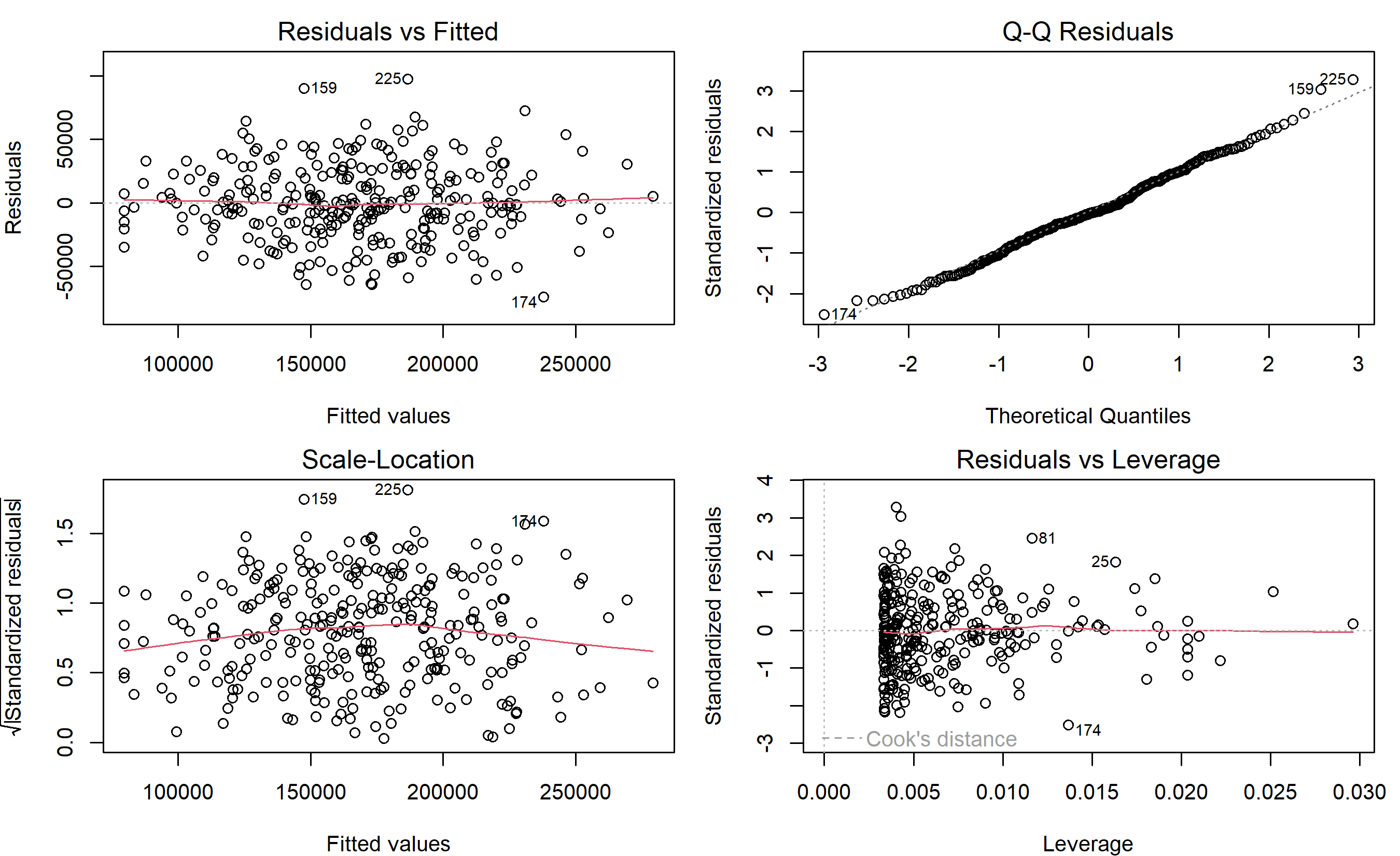
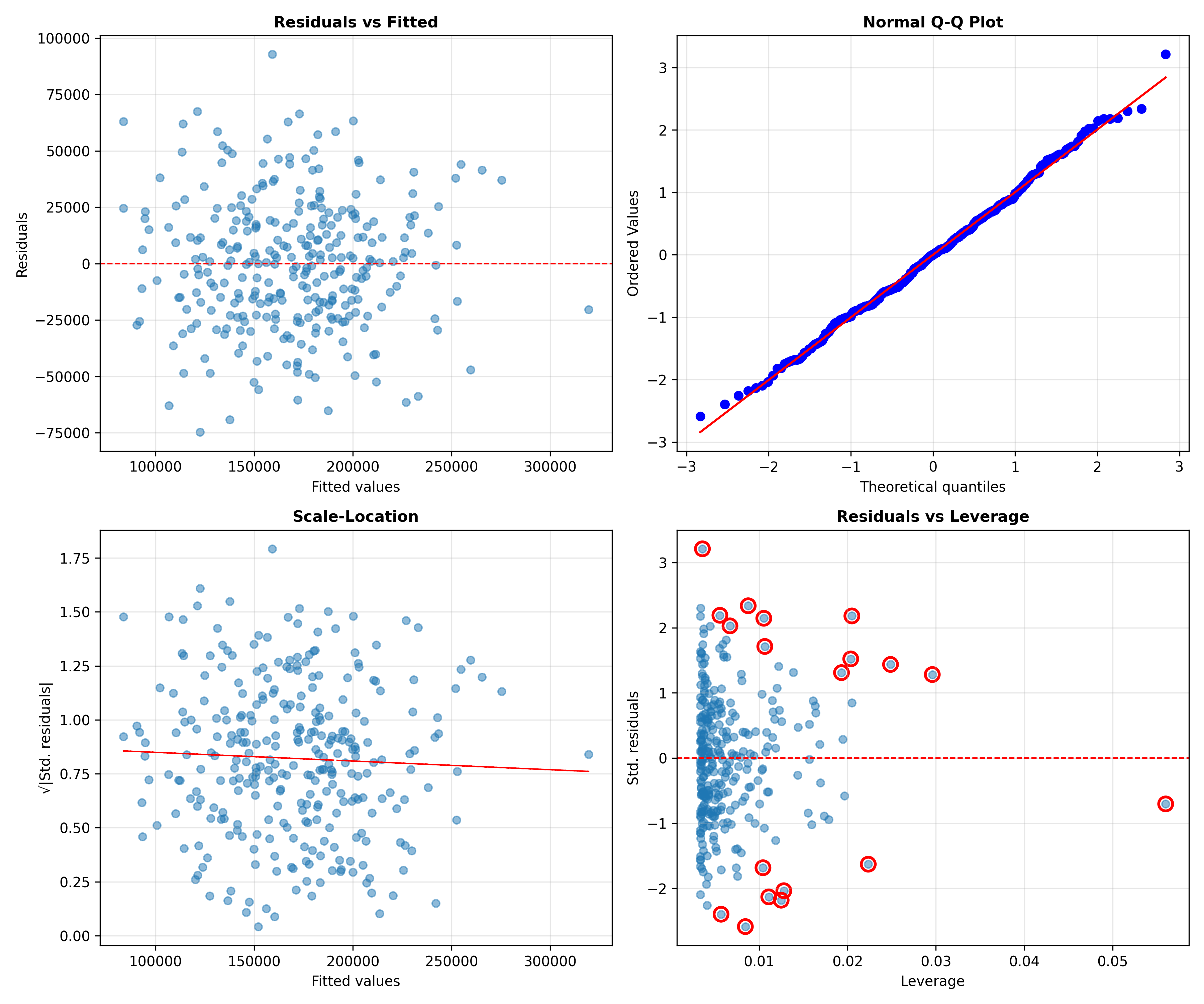
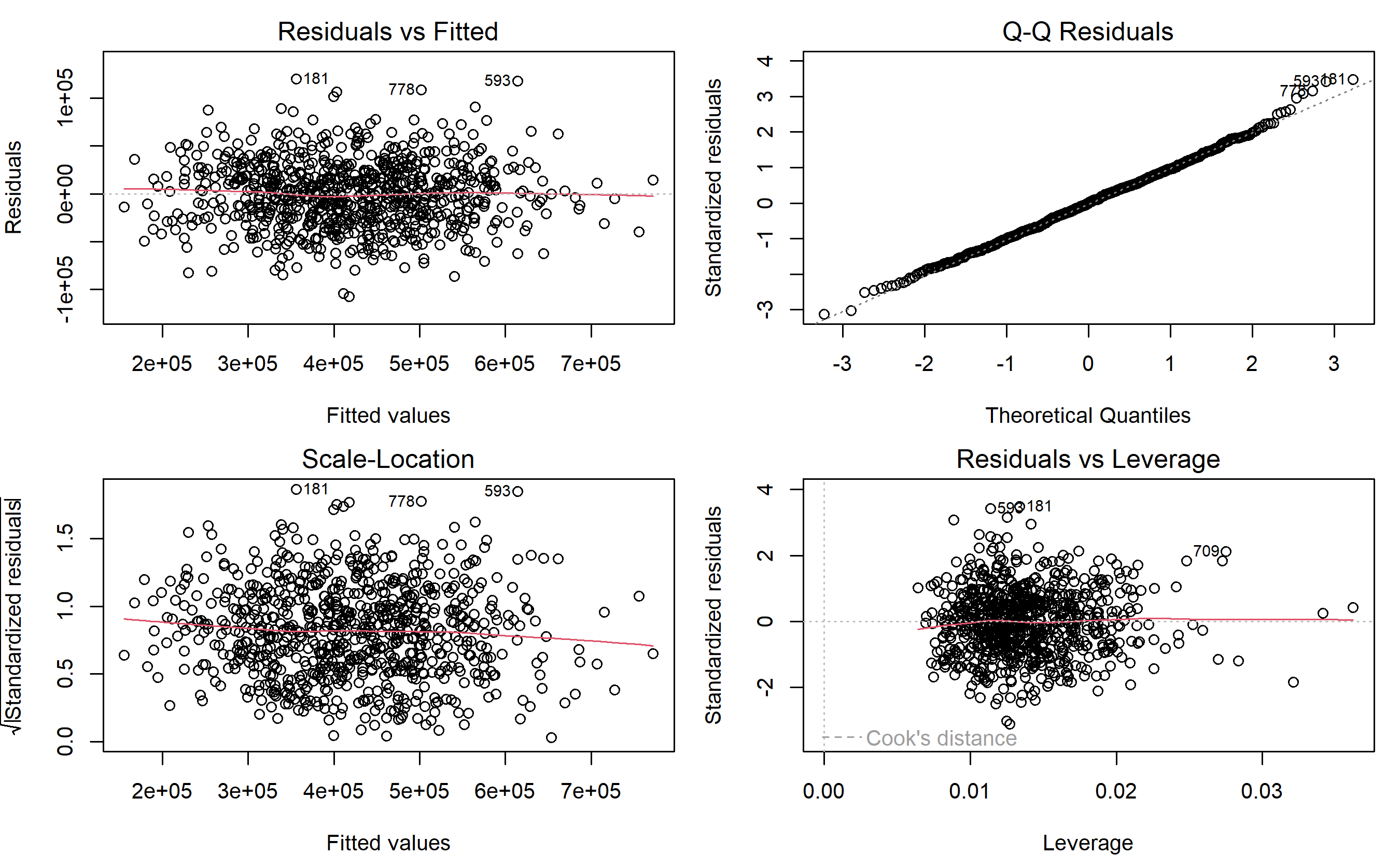
14.5.1 Four Core Diagnostic Plots

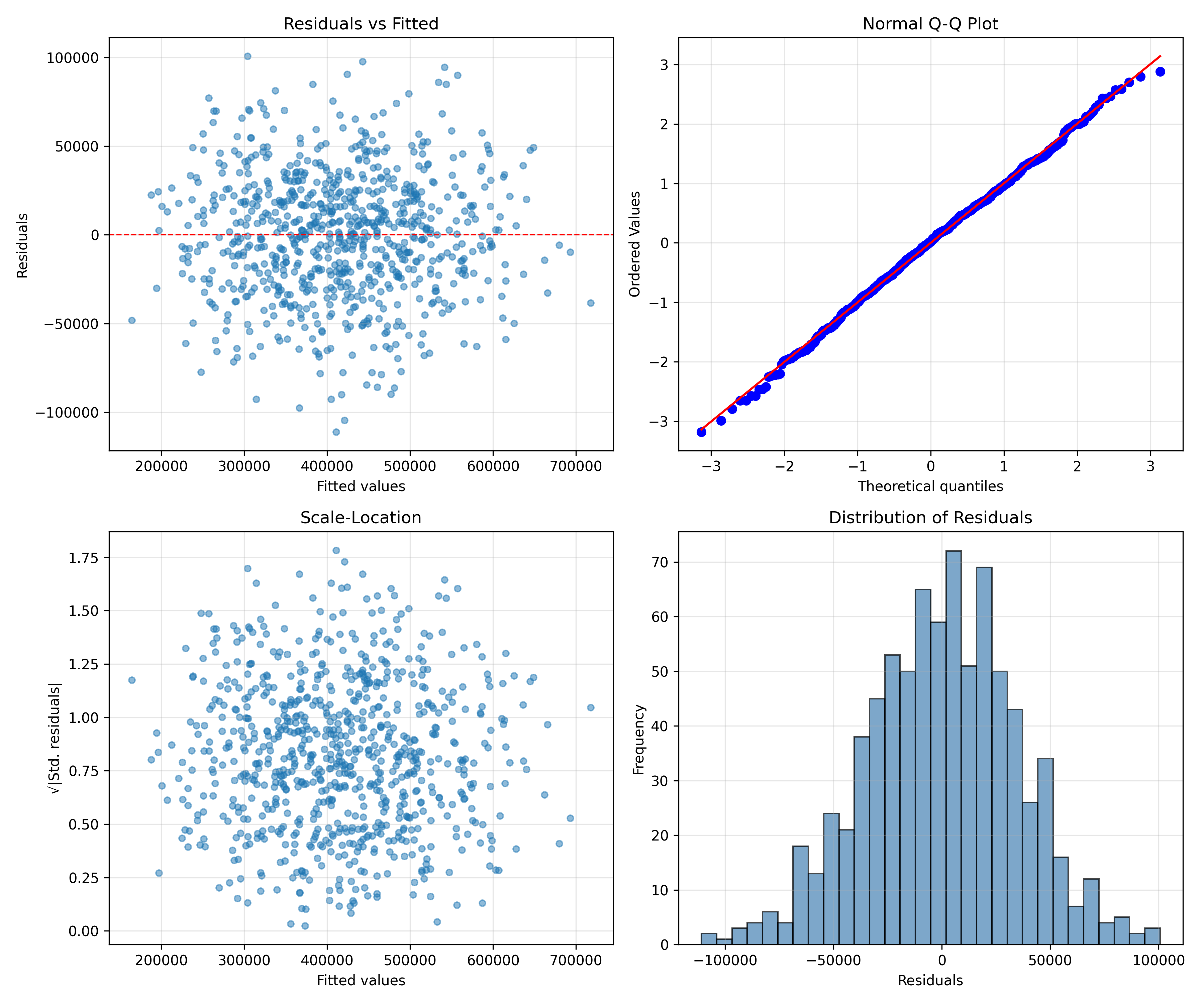
Residuals vs Fitted: Check linearity and homoscedasticity
- Should show a random scatter around y = 0 with no patterns
- If points form a U-shape or fan outward, assumptions violated
Q-Q (Quantile-Quantile) Plot: Check normality
- Points should lie on the diagonal
- Deviations in the tails indicate non-normality
Scale-Location Plot: Check homoscedasticity
- Plot of √|standardised residuals| vs fitted values
- Should show a flat trend line; upward or downward slope indicates heteroscedasticity
Residuals vs Leverage (Cook’s Distance): Identify influential points
- Outliers with high leverage can distort estimates
- Points with Cook’s D > 4/(n−p−1) are influential

14.5.2 Worked Example: Diagnostic Plots for Lagos Property Model

Show code

# Diagnostic plots for the Lagos property model

# Fit regression (from previous example)
fit <- lm(price_usd ~ size_sqft, data = lagos_property)

# Standard diagnostic plots (all four at once)
par(mfrow = c(2, 2), mar = c(4, 4, 2, 1))
plot(fit)

Show code

par(mfrow = c(1, 1))

# Interpretation of each plot
cat("Interpretation of Diagnostic Plots:\n\n")
#> Interpretation of Diagnostic Plots:

cat("1. Residuals vs Fitted Values:\n")
#> 1. Residuals vs Fitted Values:
cat("   - Points should scatter randomly around y=0\n")
#>    - Points should scatter randomly around y=0
cat("   - No funnel pattern (constant variance)\n")
#>    - No funnel pattern (constant variance)
cat("   - No U-shape or curve (linearity)\n\n")
#>    - No U-shape or curve (linearity)

cat("2. Q-Q Plot (Normal Probability Plot):\n")
#> 2. Q-Q Plot (Normal Probability Plot):
cat("   - Points should lie on the diagonal line\n")
#>    - Points should lie on the diagonal line
cat("   - Deviations in upper/lower tails indicate non-normality\n\n")
#>    - Deviations in upper/lower tails indicate non-normality

cat("3. Scale-Location Plot:\n")
#> 3. Scale-Location Plot:
cat("   - Standardised residual square root vs fitted values\n")
#>    - Standardised residual square root vs fitted values
cat("   - Should be flat if homoscedasticity holds\n")
#>    - Should be flat if homoscedasticity holds
cat("   - Upward slope indicates heteroscedasticity\n\n")
#>    - Upward slope indicates heteroscedasticity

cat("4. Residuals vs Leverage:\n")
#> 4. Residuals vs Leverage:
cat("   - Identifies influential points (high Cook's distance)\n")
#>    - Identifies influential points (high Cook's distance)
cat("   - Points in upper-right or lower-right corners are influential\n\n")
#>    - Points in upper-right or lower-right corners are influential

# Extract and examine residuals
resid_standardised <- rstandard(fit)
leverage <- hat(model.matrix(fit))
cooks_d <- cooks.distance(fit)

# Report any concerning points
problematic <- which(cooks_d > 4 / length(price_usd))
if (length(problematic) > 0) {
  cat("Observations with high influence (Cook's D):\n")
  print(problematic)
} else {
  cat("No highly influential points detected.\n")
}
#> Observations with high influence (Cook's D):
#>   9  19  25  48  81 159 162 174 225 230 246 266 287 
#>   9  19  25  48  81 159 162 174 225 230 246 266 287

# Test for normality
shapiro_test <- shapiro.test(resid_standardised)
cat("\nShapiro-Wilk Normality Test:\n")
#> 
#> Shapiro-Wilk Normality Test:
cat("p-value:", round(shapiro_test$p.value, 4), "\n")
#> p-value: 0.3841
if (shapiro_test$p.value < 0.05) {
  cat("Residuals may deviate from normality (p < 0.05)\n")
} else {
  cat("Residuals appear normally distributed (p >= 0.05)\n")
}
#> Residuals appear normally distributed (p >= 0.05)

Show code

import numpy as np
import matplotlib.pyplot as plt
from scipy import stats
from statsmodels.graphics.gofplots import ProbPlot
from statsmodels.stats.outliers_influence import OLSInfluence

# Assume model, X, y_pred, residuals are from previous example

# Standardised residuals and leverage
n = len(price_usd)
p = 1  # number of predictors
residuals_std = residuals / rmse
X_with_const = np.column_stack([np.ones(n), size_sqft])
hat_matrix = X_with_const @ np.linalg.inv(X_with_const.T @ X_with_const) @ X_with_const.T
leverage = np.diag(hat_matrix)

# Cook's distance via statsmodels OLS
sm_model = sm.OLS(price_usd, sm.add_constant(size_sqft)).fit()
influence = OLSInfluence(sm_model)
cooks_d = influence.cooks_distance[0]

# Create 2x2 subplot grid
fig, axes = plt.subplots(2, 2, figsize=(12, 10))

# Plot 1: Residuals vs Fitted
ax = axes[0, 0]
ax.scatter(y_pred, residuals, alpha=0.5, s=30)
ax.axhline(y=0, color='red', linestyle='--', linewidth=1)
ax.set_xlabel('Fitted values', fontsize=10)
ax.set_ylabel('Residuals', fontsize=10)
ax.set_title('Residuals vs Fitted', fontsize=11, fontweight='bold')
ax.grid(True, alpha=0.3)

# Plot 2: Q-Q Plot
ax = axes[0, 1]
stats.probplot(residuals_std, dist="norm", plot=ax)
#> ((array([-2.83270147, -2.5363011 , -2.36847471, -2.24887944, -2.15478411,
#>        -2.07661294, -2.00938931, -1.95018201, -1.89711324, -1.84890481,
#>        -1.80464581, -1.76366326, -1.72544529, -1.68959313, -1.65578984,
#>        -1.62377915, -1.5933508 , -1.56433003, -1.53656998, -1.50994596,
#>        -1.48435118, -1.45969344, -1.43589258, -1.41287842, -1.39058917,
#>        -1.36897015, -1.34797267, -1.32755325, -1.30767283, -1.28829622,
#>        -1.26939159, -1.25093005, -1.23288529, -1.21523328, -1.19795202,
#>        -1.1810213 , -1.16442252, -1.1481385 , -1.13215338, -1.11645243,
#>        -1.10102199, -1.08584934, -1.07092263, -1.0562308 , -1.04176348,
#>        -1.02751099, -1.01346422, -0.99961462, -0.98595415, -0.97247524,
#>        -0.95917073, -0.94603388, -0.93305829, -0.92023793, -0.90756706,
#>        -0.89504026, -0.88265235, -0.87039844, -0.85827385, -0.84627414,
#>        -0.83439507, -0.82263259, -0.81098284, -0.79944213, -0.78800692,
#>        -0.77667384, -0.76543965, -0.75430125, -0.74325565, -0.73229999,
#>        -0.72143154, -0.71064764, -0.69994576, -0.68932345, -0.67877835,
#>        -0.66830821, -0.65791081, -0.64758406, -0.63732592, -0.6271344 ,
#>        -0.61700761, -0.60694371, -0.59694091, -0.58699748, -0.57711175,
#>        -0.56728211, -0.55750697, -0.54778482, -0.53811417, -0.52849359,
#>        -0.51892168, -0.50939708, -0.49991847, -0.49048456, -0.4810941 ,
#>        -0.47174588, -0.4624387 , -0.45317141, -0.44394288, -0.434752  ,
#>        -0.42559771, -0.41647894, -0.40739467, -0.3983439 , -0.38932564,
#>        -0.38033893, -0.37138284, -0.36245644, -0.35355883, -0.34468912,
#>        -0.33584644, -0.32702995, -0.31823881, -0.30947219, -0.3007293 ,
#>        -0.29200933, -0.28331151, -0.27463506, -0.26597925, -0.25734332,
#>        -0.24872654, -0.24012818, -0.23154755, -0.22298393, -0.21443663,
#>        -0.20590496, -0.19738826, -0.18888586, -0.18039708, -0.17192129,
#>        -0.16345783, -0.15500606, -0.14656535, -0.13813507, -0.12971459,
#>        -0.12130331, -0.11290059, -0.10450584, -0.09611845, -0.08773782,
#>        -0.07936334, -0.07099442, -0.06263048, -0.05427091, -0.04591514,
#>        -0.03756257, -0.02921261, -0.0208647 , -0.01251824, -0.00417265,
#>         0.00417265,  0.01251824,  0.0208647 ,  0.02921261,  0.03756257,
#>         0.04591514,  0.05427091,  0.06263048,  0.07099442,  0.07936334,
#>         0.08773782,  0.09611845,  0.10450584,  0.11290059,  0.12130331,
#>         0.12971459,  0.13813507,  0.14656535,  0.15500606,  0.16345783,
#>         0.17192129,  0.18039708,  0.18888586,  0.19738826,  0.20590496,
#>         0.21443663,  0.22298393,  0.23154755,  0.24012818,  0.24872654,
#>         0.25734332,  0.26597925,  0.27463506,  0.28331151,  0.29200933,
#>         0.3007293 ,  0.30947219,  0.31823881,  0.32702995,  0.33584644,
#>         0.34468912,  0.35355883,  0.36245644,  0.37138284,  0.38033893,
#>         0.38932564,  0.3983439 ,  0.40739467,  0.41647894,  0.42559771,
#>         0.434752  ,  0.44394288,  0.45317141,  0.4624387 ,  0.47174588,
#>         0.4810941 ,  0.49048456,  0.49991847,  0.50939708,  0.51892168,
#>         0.52849359,  0.53811417,  0.54778482,  0.55750697,  0.56728211,
#>         0.57711175,  0.58699748,  0.59694091,  0.60694371,  0.61700761,
#>         0.6271344 ,  0.63732592,  0.64758406,  0.65791081,  0.66830821,
#>         0.67877835,  0.68932345,  0.69994576,  0.71064764,  0.72143154,
#>         0.73229999,  0.74325565,  0.75430125,  0.76543965,  0.77667384,
#>         0.78800692,  0.79944213,  0.81098284,  0.82263259,  0.83439507,
#>         0.84627414,  0.85827385,  0.87039844,  0.88265235,  0.89504026,
#>         0.90756706,  0.92023793,  0.93305829,  0.94603388,  0.95917073,
#>         0.97247524,  0.98595415,  0.99961462,  1.01346422,  1.02751099,
#>         1.04176348,  1.0562308 ,  1.07092263,  1.08584934,  1.10102199,
#>         1.11645243,  1.13215338,  1.1481385 ,  1.16442252,  1.1810213 ,
#>         1.19795202,  1.21523328,  1.23288529,  1.25093005,  1.26939159,
#>         1.28829622,  1.30767283,  1.32755325,  1.34797267,  1.36897015,
#>         1.39058917,  1.41287842,  1.43589258,  1.45969344,  1.48435118,
#>         1.50994596,  1.53656998,  1.56433003,  1.5933508 ,  1.62377915,
#>         1.65578984,  1.68959313,  1.72544529,  1.76366326,  1.80464581,
#>         1.84890481,  1.89711324,  1.95018201,  2.00938931,  2.07661294,
#>         2.15478411,  2.24887944,  2.36847471,  2.5363011 ,  2.83270147]), array([-2.58771519e+00, -2.39778087e+00, -2.25818029e+00, -2.18226552e+00,
#>        -2.13155397e+00, -2.09355721e+00, -2.03697912e+00, -1.93660966e+00,
#>        -1.82245885e+00, -1.81395099e+00, -1.74674477e+00, -1.71827629e+00,
#>        -1.69595160e+00, -1.68436912e+00, -1.68409359e+00, -1.66604964e+00,
#>        -1.62977619e+00, -1.56914078e+00, -1.55435109e+00, -1.51111965e+00,
#>        -1.49823498e+00, -1.45460183e+00, -1.42976962e+00, -1.42270341e+00,
#>        -1.40224471e+00, -1.39208442e+00, -1.37398089e+00, -1.32351180e+00,
#>        -1.26177018e+00, -1.25873911e+00, -1.23500848e+00, -1.19872625e+00,
#>        -1.15524767e+00, -1.14685957e+00, -1.10373538e+00, -1.08646033e+00,
#>        -1.07553131e+00, -1.06742723e+00, -1.04198818e+00, -1.03625815e+00,
#>        -1.02571729e+00, -1.01983418e+00, -1.01511323e+00, -1.00152098e+00,
#>        -1.00079146e+00, -1.00063889e+00, -9.86062935e-01, -9.83491152e-01,
#>        -9.43218690e-01, -9.16498895e-01, -9.07476230e-01, -8.97333572e-01,
#>        -8.92960858e-01, -8.89014412e-01, -8.87750319e-01, -8.85173156e-01,
#>        -8.57733230e-01, -8.56947612e-01, -8.44061340e-01, -8.39610855e-01,
#>        -8.27768220e-01, -8.26599854e-01, -8.25218798e-01, -8.21199427e-01,
#>        -8.17315277e-01, -8.05593590e-01, -8.03512531e-01, -8.02395723e-01,
#>        -7.94887568e-01, -7.87245373e-01, -7.71262491e-01, -7.45634995e-01,
#>        -7.44485290e-01, -7.18569938e-01, -7.11786499e-01, -7.04283039e-01,
#>        -7.02362394e-01, -6.63456436e-01, -6.41656478e-01, -6.32533142e-01,
#>        -6.15186350e-01, -6.02521529e-01, -5.95001351e-01, -5.90712643e-01,
#>        -5.87971005e-01, -5.87638581e-01, -5.78785674e-01, -5.74771121e-01,
#>        -5.64970884e-01, -5.64463583e-01, -5.58742635e-01, -5.56266695e-01,
#>        -5.46709334e-01, -5.42170715e-01, -5.37429184e-01, -5.32011327e-01,
#>        -5.19365719e-01, -5.18091548e-01, -5.16912898e-01, -5.16898917e-01,
#>        -5.14932114e-01, -4.92953236e-01, -4.91311793e-01, -4.60211801e-01,
#>        -4.52071611e-01, -4.50892529e-01, -4.45782349e-01, -4.39269919e-01,
#>        -4.22668934e-01, -4.10369686e-01, -3.87511666e-01, -3.85581585e-01,
#>        -3.80961502e-01, -3.70516491e-01, -3.52629871e-01, -3.46367140e-01,
#>        -3.38167376e-01, -2.95160845e-01, -2.94900503e-01, -2.88816639e-01,
#>        -2.88467617e-01, -2.61866664e-01, -2.26111349e-01, -2.20202434e-01,
#>        -2.11729922e-01, -2.07030765e-01, -2.04889210e-01, -1.92563278e-01,
#>        -1.92056626e-01, -1.86554701e-01, -1.73684532e-01, -1.69925885e-01,
#>        -1.68458203e-01, -1.62900010e-01, -1.29843201e-01, -1.22115336e-01,
#>        -1.19367251e-01, -1.06836605e-01, -9.64540243e-02, -8.83564059e-02,
#>        -7.89803097e-02, -6.36854305e-02, -6.01927253e-02, -4.46802237e-02,
#>        -3.38845916e-02, -2.66280206e-02, -2.27058271e-02, -1.17004824e-02,
#>        -7.66383749e-03, -1.76009690e-03,  1.04086255e-02,  1.56479112e-02,
#>         2.42370693e-02,  3.40993099e-02,  3.47137100e-02,  3.91355016e-02,
#>         4.27155144e-02,  6.06175183e-02,  6.76067687e-02,  7.09967230e-02,
#>         8.68757210e-02,  8.93134844e-02,  9.10062785e-02,  9.25635278e-02,
#>         9.40529190e-02,  1.00614307e-01,  1.01087885e-01,  1.08330347e-01,
#>         1.10305223e-01,  1.19135957e-01,  1.35927687e-01,  1.36630103e-01,
#>         1.54250918e-01,  1.56437951e-01,  1.60791491e-01,  1.75053114e-01,
#>         2.02203845e-01,  2.11008960e-01,  2.15540481e-01,  2.37885458e-01,
#>         2.50803992e-01,  2.52580514e-01,  2.66792382e-01,  2.72717652e-01,
#>         2.74157066e-01,  2.81561394e-01,  2.86869676e-01,  2.90509794e-01,
#>         3.19195027e-01,  3.23231251e-01,  3.23529681e-01,  3.26905451e-01,
#>         3.56801959e-01,  3.59325149e-01,  3.60734412e-01,  3.69325569e-01,
#>         3.77997871e-01,  3.97188941e-01,  3.97244786e-01,  3.99065098e-01,
#>         4.03182690e-01,  4.04221990e-01,  4.09805084e-01,  4.29373024e-01,
#>         4.36599726e-01,  4.47831052e-01,  4.70463429e-01,  4.99018453e-01,
#>         5.15304385e-01,  5.20603534e-01,  5.44856467e-01,  5.54103202e-01,
#>         5.54178116e-01,  5.57920596e-01,  5.67680266e-01,  5.74027594e-01,
#>         5.90601428e-01,  5.94176145e-01,  5.95819053e-01,  6.04971168e-01,
#>         6.21730335e-01,  6.32588886e-01,  6.44504618e-01,  6.49388909e-01,
#>         6.59825003e-01,  6.64728454e-01,  6.83678979e-01,  6.89474426e-01,
#>         6.93559368e-01,  6.94856100e-01,  7.10375197e-01,  7.13557993e-01,
#>         7.14940055e-01,  7.35888601e-01,  7.45707241e-01,  7.68060986e-01,
#>         7.84509224e-01,  7.99601287e-01,  8.01841556e-01,  8.05783276e-01,
#>         8.21585130e-01,  8.33940983e-01,  8.49138626e-01,  8.49289060e-01,
#>         8.58035155e-01,  8.62367314e-01,  8.76467458e-01,  8.84495869e-01,
#>         8.88358134e-01,  8.89284121e-01,  8.94851756e-01,  9.31591200e-01,
#>         9.81920458e-01,  9.90862558e-01,  9.97133094e-01,  1.02681953e+00,
#>         1.04421931e+00,  1.06444617e+00,  1.07428469e+00,  1.11278793e+00,
#>         1.12536084e+00,  1.14723968e+00,  1.18458749e+00,  1.19681175e+00,
#>         1.23364129e+00,  1.26120542e+00,  1.28176234e+00,  1.28789537e+00,
#>         1.29986494e+00,  1.31064409e+00,  1.31733030e+00,  1.40554578e+00,
#>         1.43689083e+00,  1.43798992e+00,  1.45433503e+00,  1.52170536e+00,
#>         1.52851199e+00,  1.54128512e+00,  1.55039465e+00,  1.55052033e+00,
#>         1.59005283e+00,  1.60796188e+00,  1.61069245e+00,  1.63243922e+00,
#>         1.68637708e+00,  1.71292345e+00,  1.74093115e+00,  1.74492136e+00,
#>         1.81354753e+00,  1.91323620e+00,  1.98294793e+00,  2.02570731e+00,
#>         2.02873971e+00,  2.14540222e+00,  2.17614442e+00,  2.18107842e+00,
#>         2.19106946e+00,  2.30034631e+00,  2.33724981e+00,  3.21127941e+00])), (np.float64(1.0031675375811913), np.float64(-4.263256414560601e-16), np.float64(0.9985814744552876)))
ax.set_title('Normal Q-Q Plot', fontsize=11, fontweight='bold')
ax.grid(True, alpha=0.3)

# Plot 3: Scale-Location (sqrt(|std residuals|) vs fitted)
ax = axes[1, 0]
sqrt_std_resid = np.sqrt(np.abs(residuals_std))
ax.scatter(y_pred, sqrt_std_resid, alpha=0.5, s=30)
ax.set_xlabel('Fitted values', fontsize=10)
ax.set_ylabel('√|Std. residuals|', fontsize=10)
ax.set_title('Scale-Location', fontsize=11, fontweight='bold')
# Add trend line
z = np.polyfit(y_pred, sqrt_std_resid, 1)
p_fit = np.poly1d(z)
ax.plot(y_pred, p_fit(y_pred), 'r--', linewidth=1)
ax.grid(True, alpha=0.3)

# Plot 4: Residuals vs Leverage (with Cook's distance)
ax = axes[1, 1]
ax.scatter(leverage, residuals_std, alpha=0.5, s=30)
ax.axhline(y=0, color='red', linestyle='--', linewidth=1)
# Highlight high-leverage/high-residual points
threshold = 4 / (n - p - 1)
problematic = cooks_d > threshold
ax.scatter(leverage[problematic], residuals_std[problematic], color='red', s=100,
           marker='o', facecolors='none', edgecolors='red', linewidth=2)
ax.set_xlabel('Leverage', fontsize=10)
ax.set_ylabel('Std. residuals', fontsize=10)
ax.set_title('Residuals vs Leverage', fontsize=11, fontweight='bold')
ax.grid(True, alpha=0.3)

plt.tight_layout()
plt.savefig('diagnostic_plots.png', dpi=300, bbox_inches='tight')
plt.show()

Show code


# Test for normality (Shapiro-Wilk)
shapiro_stat, shapiro_p = stats.shapiro(residuals_std)
print(f"Shapiro-Wilk Normality Test:")
#> Shapiro-Wilk Normality Test:
print(f"  Test statistic: {shapiro_stat:.4f}")
#>   Test statistic: 0.9969
print(f"  p-value: {shapiro_p:.4f}")
#>   p-value: 0.8255
if shapiro_p < 0.05:
    print("  Residuals may deviate from normality (p < 0.05)")
else:
    print("  Residuals appear normally distributed (p >= 0.05)")
#>   Residuals appear normally distributed (p >= 0.05)

# Report influential points
if problematic.sum() > 0:
    print(f"\nObservations with high influence (Cook's D > {threshold:.4f}):")
    print(f"  Indices: {np.where(problematic)[0].tolist()}")
else:
    print("\nNo highly influential points detected.")
#> 
#> Observations with high influence (Cook's D > 0.0134):
#>   Indices: [23, 74, 82, 100, 113, 120, 125, 142, 160, 171, 178, 179, 209, 220, 244, 252, 266, 271, 283]

📝 Section 9.5 Review Questions

If the residuals vs fitted plot shows a strong upward fan pattern, which assumption is violated?
What does a point far above the Q-Q line in the upper tail indicate?
How would you respond to an influential outlier: (a) delete it, (b) downweight it, (c) investigate why it’s unusual?
Why are diagnostic plots crucial before reporting a regression model to stakeholders?

14.6 Multiple Linear Regression

Multiple regression adds p > 1 predictors, allowing us to estimate partial effects (holding other variables constant).

14.6.1 Model and Matrix Form

The multiple regression model is: \[Y_i = \beta_0 + \beta_1 X_{i,1} + \beta_2 X_{i,2} + \cdots + \beta_p X_{i,p} + \varepsilon_i\]

In matrix notation: \[\mathbf{y} = \mathbf{X}\boldsymbol{\beta} + \boldsymbol{\varepsilon}\]

where y is n×1, X is n×(p+1) (with a column of 1s for the intercept), β is (p+1)×1, ε is n×1.

The OLS solution is: \[\hat{\boldsymbol{\beta}} = (\mathbf{X}^T \mathbf{X})^{-1} \mathbf{X}^T \mathbf{y}\]

📘 Theory: Partial Slopes and Multicollinearity

A coefficient β̂_j represents the change in Y per unit change in X_j, holding all other predictors constant.

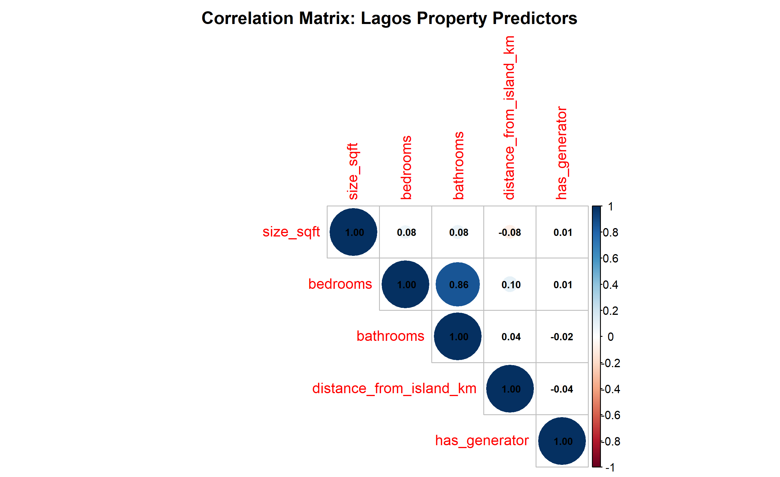
Multicollinearity: If two predictors are highly correlated, their regression coefficients become unstable: - Large standard errors → wide confidence intervals → low power - Coefficients are sensitive to small changes in data or model specification - The partial slope β̂_j is ill-defined when X_j and X_k are nearly linearly dependent

Variance Inflation Factor (VIF): Measures how much multicollinearity inflates the standard error of β̂_j: \[\text{VIF}_j = \frac{1}{1 - R_j^2}\]

where R_j² is the R² from regressing X_j on all other X’s.

VIF = 1: no collinearity
VIF > 5–10: concerning multicollinearity (coefficients unreliable)

14.6.2 Worked Example: Lagos Property Prices with Multiple Predictors

Show code

# Multiple regression: Lagos property prices

set.seed(42)
n <- 300

# Predictors
size_sqft <- rnorm(n, 1500, 500)
size_sqft <- pmax(size_sqft, 400)
bedrooms <- rpois(n, 3) + 1
bathrooms <- bedrooms - rpois(n, 1)
bathrooms <- pmax(bathrooms, 1)
distance_from_island_km <- rnorm(n, 15, 8)
distance_from_island_km <- pmax(distance_from_island_km, 0.5)
has_generator <- rbinom(n, 1, prob = 0.6)

# Outcome: price (function of predictors)
price_usd <- 30000 +
             75 * size_sqft +
             15000 * bedrooms +
             8000 * bathrooms -
             500 * distance_from_island_km +
             20000 * has_generator +
             rnorm(n, 0, 25000)

lagos_multi <- tibble(
  size_sqft, bedrooms, bathrooms, distance_from_island_km, has_generator, price_usd
)

# Fit multiple regression
fit_multi <- lm(price_usd ~ size_sqft + bedrooms + bathrooms +
                distance_from_island_km + has_generator,
                data = lagos_multi)

# Summary
summary(fit_multi)
#> 
#> Call:
#> lm(formula = price_usd ~ size_sqft + bedrooms + bathrooms + distance_from_island_km + 
#>     has_generator, data = lagos_multi)
#> 
#> Residuals:
#>    Min     1Q Median     3Q    Max 
#> -63772 -16228   -250  15536  71100 
#> 
#> Coefficients:
#>                          Estimate Std. Error t value Pr(>|t|)    
#> (Intercept)             31054.469   6373.621   4.872 1.81e-06 ***
#> size_sqft                  77.183      2.916  26.469  < 2e-16 ***
#> bedrooms                18564.032   1709.898  10.857  < 2e-16 ***
#> bathrooms                3920.835   1645.944   2.382   0.0178 *  
#> distance_from_island_km  -899.902    190.660  -4.720 3.65e-06 ***
#> has_generator           20291.622   2817.624   7.202 5.00e-12 ***
#> ---
#> Signif. codes:  0 '***' 0.001 '**' 0.01 '*' 0.05 '.' 0.1 ' ' 1
#> 
#> Residual standard error: 24240 on 294 degrees of freedom
#> Multiple R-squared:  0.8413, Adjusted R-squared:  0.8386 
#> F-statistic: 311.7 on 5 and 294 DF,  p-value: < 2.2e-16

# Variance Inflation Factors (VIF)
car::vif(fit_multi)
#>               size_sqft                bedrooms               bathrooms 
#>                1.014934                3.912869                3.879538 
#> distance_from_island_km           has_generator 
#>                1.029787                1.005439

# Correlations among predictors
cor_matrix <- cor(lagos_multi[, -6])
corrplot::corrplot(cor_matrix, method = "circle", type = "upper",
                   addCoef.col = "black", number.cex = 0.7,
                   title = "Correlation Matrix: Lagos Property Predictors",
                   mar = c(0, 0, 2, 0))

Show code


# Model comparison: simple vs multiple
fit_simple <- lm(price_usd ~ size_sqft, data = lagos_multi)

cat("Model Comparison:\n\n")
#> Model Comparison:
cat("Simple (size only):\n")
#> Simple (size only):
cat("  R² =", round(summary(fit_simple)$r.squared, 4), "\n")
#>   R² = 0.4602
cat("  Adj R² =", round(summary(fit_simple)$adj.r.squared, 4), "\n\n")
#>   Adj R² = 0.4583

cat("Multiple (all predictors):\n")
#> Multiple (all predictors):
cat("  R² =", round(summary(fit_multi)$r.squared, 4), "\n")
#>   R² = 0.8413
cat("  Adj R² =", round(summary(fit_multi)$adj.r.squared, 4), "\n\n")
#>   Adj R² = 0.8386

# Predicted values for a "typical" property
new_property <- tibble(
  size_sqft = 1500,
  bedrooms = 3,
  bathrooms = 2,
  distance_from_island_km = 12,
  has_generator = 1
)

prediction <- predict(fit_multi, newdata = new_property,
                     interval = "confidence", level = 0.95)
cat("Predicted price for typical property:\n")
#> Predicted price for typical property:
print(prediction)
#>        fit      lwr      upr
#> 1 219855.6 215632.7 224078.6

Show code

import numpy as np
import pandas as pd
from sklearn.linear_model import LinearRegression
from scipy import stats
import statsmodels.api as sm
from statsmodels.stats.outliers_influence import variance_inflation_factor

np.random.seed(42)
n = 300

# Predictors
size_sqft = np.random.normal(1500, 500, n)
size_sqft = np.maximum(size_sqft, 400)
bedrooms = np.random.poisson(3, n) + 1
bathrooms = bedrooms - np.random.poisson(1, n)
bathrooms = np.maximum(bathrooms, 1)
distance_km = np.random.normal(15, 8, n)
distance_km = np.maximum(distance_km, 0.5)
has_generator = np.random.binomial(1, 0.6, n)

# Outcome
price_usd = (30000 + 75 * size_sqft + 15000 * bedrooms + 8000 * bathrooms -
             500 * distance_km + 20000 * has_generator +
             np.random.normal(0, 25000, n))

# Create data frame
lagos_multi = pd.DataFrame({
    'size_sqft': size_sqft,
    'bedrooms': bedrooms,
    'bathrooms': bathrooms,
    'distance_km': distance_km,
    'has_generator': has_generator,
    'price_usd': price_usd
})

# Fit using statsmodels for comprehensive output
X = sm.add_constant(lagos_multi[['size_sqft', 'bedrooms', 'bathrooms', 'distance_km', 'has_generator']])
fit_multi = sm.OLS(lagos_multi['price_usd'], X).fit()
print(fit_multi.summary())
#>                             OLS Regression Results                            
#> ==============================================================================
#> Dep. Variable:              price_usd   R-squared:                       0.832
#> Model:                            OLS   Adj. R-squared:                  0.829
#> Method:                 Least Squares   F-statistic:                     290.5
#> Date:                Sun, 12 Apr 2026   Prob (F-statistic):          1.86e-111
#> Time:                        14:14:31   Log-Likelihood:                -3462.0
#> No. Observations:                 300   AIC:                             6936.
#> Df Residuals:                     294   BIC:                             6958.
#> Df Model:                           5                                         
#> Covariance Type:            nonrobust                                         
#> =================================================================================
#>                     coef    std err          t      P>|t|      [0.025      0.975]
#> ---------------------------------------------------------------------------------
#> const          3.939e+04   6697.047      5.882      0.000    2.62e+04    5.26e+04
#> size_sqft        72.3376      3.001     24.108      0.000      66.432      78.243
#> bedrooms       1.093e+04   1732.018      6.312      0.000    7523.239    1.43e+04
#> bathrooms      1.106e+04   1688.410      6.548      0.000    7732.728    1.44e+04
#> distance_km    -542.8305    185.310     -2.929      0.004    -907.534    -178.128
#> has_generator  2.218e+04   2986.678      7.427      0.000    1.63e+04    2.81e+04
#> ==============================================================================
#> Omnibus:                        3.302   Durbin-Watson:                   1.947
#> Prob(Omnibus):                  0.192   Jarque-Bera (JB):                3.191
#> Skew:                          -0.201   Prob(JB):                        0.203
#> Kurtosis:                       2.694   Cond. No.                     7.37e+03
#> ==============================================================================
#> 
#> Notes:
#> [1] Standard Errors assume that the covariance matrix of the errors is correctly specified.
#> [2] The condition number is large, 7.37e+03. This might indicate that there are
#> strong multicollinearity or other numerical problems.

# Compute VIF
vif_data = pd.DataFrame()
vif_data["Variable"] = lagos_multi[['size_sqft', 'bedrooms', 'bathrooms', 'distance_km', 'has_generator']].columns
vif_data["VIF"] = [variance_inflation_factor(
    lagos_multi[['size_sqft', 'bedrooms', 'bathrooms', 'distance_km', 'has_generator']].values, i)
    for i in range(len(vif_data))]
print("\nVariance Inflation Factors:")
#> 
#> Variance Inflation Factors:
print(vif_data)
#>         Variable        VIF
#> 0      size_sqft   5.587534
#> 1       bedrooms  23.384035
#> 2      bathrooms  17.128538
#> 3    distance_km   3.630697
#> 4  has_generator   2.422596

# Model comparison
fit_simple = sm.OLS(lagos_multi['price_usd'],
                    sm.add_constant(lagos_multi['size_sqft'])).fit()

print("\n\nModel Comparison:")
#> 
#> 
#> Model Comparison:
print(f"Simple (size only):")
#> Simple (size only):
print(f"  R² = {fit_simple.rsquared:.4f}")
#>   R² = 0.3681
print(f"  Adj R² = {fit_simple.rsquared_adj:.4f}")
#>   Adj R² = 0.3660
print(f"\nMultiple (all predictors):")
#> 
#> Multiple (all predictors):
print(f"  R² = {fit_multi.rsquared:.4f}")
#>   R² = 0.8316
print(f"  Adj R² = {fit_multi.rsquared_adj:.4f}")
#>   Adj R² = 0.8288

# Prediction for a typical property
new_property = pd.DataFrame({
    'const': 1,
    'size_sqft': [1500],
    'bedrooms': [3],
    'bathrooms': [2],
    'distance_km': [12],
    'has_generator': [1]
})

pred_result = fit_multi.get_prediction(new_property)
pred_summary = pred_result.summary_frame(alpha=0.05)
print("\nPredicted price for typical property:")
#> 
#> Predicted price for typical property:
print(f"  Point estimate: ${pred_summary['mean'].values[0]:,.0f}")
#>   Point estimate: $218,473
print(f"  95% CI: [${pred_summary['mean_ci_lower'].values[0]:,.0f}, ${pred_summary['mean_ci_upper'].values[0]:,.0f}]")
#>   95% CI: [$214,244, $222,702]

Interpretation of coefficients:

Size: $75 per sq ft, holding bedrooms, bathrooms, distance, generator constant
Bedrooms: $15,000 per room, holding other factors constant (larger houses have more bedrooms, so this captures quality/amenities not fully captured by size)
Distance: −$500 per km from island (location premium for proximity to business district)
Generator: +$20,000 for having a generator (essential in power-unstable regions)

Multicollinearity check: VIF values near 1 suggest low collinearity. Bedrooms and bathrooms may be correlated (VIF ~3–4) but acceptable.

📝 Section 9.6 Review Questions

Why does adding bedrooms and bathrooms to the model change the size coefficient from 80 to 75?
If two predictors have VIF = 8, should you remove one? What are the trade-offs?
Interpret the coefficient for distance_from_island: −500. Does this make business sense?
In the prediction for a typical property, why is the 95% CI wide?

14.7 Model Evaluation and Selection

Choosing between competing models requires balancing fit and complexity.

📘 Theory: Information Criteria

Akaike Information Criterion (AIC): \[\text{AIC} = 2p - 2 \log(\hat{L})\]

where p is the number of parameters and $\hat{L}$ is the maximum likelihood.

Lower AIC is better. AIC penalises model complexity.

Bayesian Information Criterion (BIC): \[\text{BIC} = p \log(n) - 2 \log(\hat{L})\]

BIC applies a stronger penalty for complexity (log n), preferred when p is large.

Cross-Validation (CV): Divide data into k folds, fit on k−1 folds, evaluate on 1 fold, repeat k times. Report average error. - k = 5 or 10 most common - Avoids overfitting by testing on held-out data

14.7.1 Worked Example: Cross-Validation for Lagos Property Model

Show code

# 5-fold cross-validation for model selection

library(caret)

# Use k-fold cross-validation to compare models
ctrl <- trainControl(method = "cv", number = 5)

# Model 1: Size only
fit_cv_1 <- train(price_usd ~ size_sqft,
                   data = lagos_multi,
                   method = "lm",
                   trControl = ctrl)

# Model 2: Size + bedrooms + bathrooms
fit_cv_2 <- train(price_usd ~ size_sqft + bedrooms + bathrooms,
                   data = lagos_multi,
                   method = "lm",
                   trControl = ctrl)

# Model 3: All predictors
fit_cv_3 <- train(price_usd ~ size_sqft + bedrooms + bathrooms +
                   distance_from_island_km + has_generator,
                   data = lagos_multi,
                   method = "lm",
                   trControl = ctrl)

# Compare
results_cv <- resamples(list(Model_1 = fit_cv_1,
                             Model_2 = fit_cv_2,
                             Model_3 = fit_cv_3))

summary(results_cv)
#> 
#> Call:
#> summary.resamples(object = results_cv)
#> 
#> Models: Model_1, Model_2, Model_3 
#> Number of resamples: 5 
#> 
#> MAE 
#>             Min.  1st Qu.   Median     Mean  3rd Qu.     Max. NA's
#> Model_1 32810.33 34182.51 35252.18 35587.57 36701.39 38991.44    0
#> Model_2 18976.60 19075.11 21356.75 21630.11 23430.83 25311.26    0
#> Model_3 17700.55 18030.90 18243.90 19621.81 20953.30 23180.38    0
#> 
#> RMSE 
#>             Min.  1st Qu.   Median     Mean  3rd Qu.     Max. NA's
#> Model_1 40877.40 41579.82 42095.37 44323.43 47635.78 49428.79    0
#> Model_2 24118.29 24639.67 27784.45 27328.26 29220.56 30878.33    0
#> Model_3 22063.65 23121.02 24616.58 24626.07 24691.90 28637.22    0
#> 
#> Rsquared 
#>              Min.   1st Qu.    Median      Mean   3rd Qu.      Max. NA's
#> Model_1 0.3130996 0.4206385 0.4961148 0.4638775 0.5368652 0.5526691    0
#> Model_2 0.7581762 0.7694090 0.7863848 0.8011906 0.8321624 0.8598207    0
#> Model_3 0.8011644 0.8350851 0.8513225 0.8417771 0.8580778 0.8632356    0

# AIC and BIC for each model
fit_1 <- lm(price_usd ~ size_sqft, data = lagos_multi)
fit_2 <- lm(price_usd ~ size_sqft + bedrooms + bathrooms, data = lagos_multi)
fit_3 <- lm(price_usd ~ size_sqft + bedrooms + bathrooms +
            distance_from_island_km + has_generator, data = lagos_multi)

cat("\nInformation Criteria:\n\n")
#> 
#> Information Criteria:
cat("Model 1 (Size):\n")
#> Model 1 (Size):
cat("  AIC =", round(AIC(fit_1), 0), "\n")
#>   AIC = 7276
cat("  BIC =", round(BIC(fit_1), 0), "\n")
#>   BIC = 7287
cat("  RMSE (CV) =", round(fit_cv_1$results$RMSE, 0), "\n\n")
#>   RMSE (CV) = 44323

cat("Model 2 (Size + Beds + Baths):\n")
#> Model 2 (Size + Beds + Baths):
cat("  AIC =", round(AIC(fit_2), 0), "\n")
#>   AIC = 6983
cat("  BIC =", round(BIC(fit_2), 0), "\n")
#>   BIC = 7001
cat("  RMSE (CV) =", round(fit_cv_2$results$RMSE, 0), "\n\n")
#>   RMSE (CV) = 27328

cat("Model 3 (All predictors):\n")
#> Model 3 (All predictors):
cat("  AIC =", round(AIC(fit_3), 0), "\n")
#>   AIC = 6917
cat("  BIC =", round(BIC(fit_3), 0), "\n")
#>   BIC = 6943
cat("  RMSE (CV) =", round(fit_cv_3$results$RMSE, 0), "\n")
#>   RMSE (CV) = 24626

Show code

from sklearn.model_selection import cross_val_score, KFold
from sklearn.linear_model import LinearRegression
import numpy as np

# Prepare data
X1 = lagos_multi[['size_sqft']].values
X2 = lagos_multi[['size_sqft', 'bedrooms', 'bathrooms']].values
X3 = lagos_multi[['size_sqft', 'bedrooms', 'bathrooms', 'distance_km', 'has_generator']].values
y = lagos_multi['price_usd'].values

# 5-fold cross-validation
kfold = KFold(n_splits=5, shuffle=True, random_state=42)

# Model 1: Size only
model1 = LinearRegression()
cv_scores_1 = cross_val_score(model1, X1, y, cv=kfold, scoring='neg_mean_squared_error')
rmse_1 = np.sqrt(-cv_scores_1.mean())

# Model 2: Size + Beds + Baths
model2 = LinearRegression()
cv_scores_2 = cross_val_score(model2, X2, y, cv=kfold, scoring='neg_mean_squared_error')
rmse_2 = np.sqrt(-cv_scores_2.mean())

# Model 3: All predictors
model3 = LinearRegression()
cv_scores_3 = cross_val_score(model3, X3, y, cv=kfold, scoring='neg_mean_squared_error')
rmse_3 = np.sqrt(-cv_scores_3.mean())

# AIC and BIC
def compute_aic_bic(n, k, ss_res):
    rmse = np.sqrt(ss_res / (n - k - 1))
    aic = n * np.log(ss_res / n) + 2 * (k + 1)
    bic = n * np.log(ss_res / n) + (k + 1) * np.log(n)
    return aic, bic

# Fit models and compute residual SS
model1.fit(X1, y)

LinearRegression()

Show code

ss_res_1 = np.sum((y - model1.predict(X1))**2)
aic_1, bic_1 = compute_aic_bic(len(y), 1, ss_res_1)

model2.fit(X2, y)

LinearRegression()

Show code

ss_res_2 = np.sum((y - model2.predict(X2))**2)
aic_2, bic_2 = compute_aic_bic(len(y), 3, ss_res_2)

model3.fit(X3, y)

LinearRegression()

Show code

ss_res_3 = np.sum((y - model3.predict(X3))**2)
aic_3, bic_3 = compute_aic_bic(len(y), 5, ss_res_3)

print("Model Comparison:\n")
#> Model Comparison:
print("Model 1 (Size only):")
#> Model 1 (Size only):
print(f"  AIC = {aic_1:,.0f}")
#>   AIC = 6,473
print(f"  BIC = {bic_1:,.0f}")
#>   BIC = 6,481
print(f"  CV RMSE = ${rmse_1:,.0f}\n")
#>   CV RMSE = $48,401

print("Model 2 (Size + Bedrooms + Bathrooms):")
#> Model 2 (Size + Bedrooms + Bathrooms):
print(f"  AIC = {aic_2:,.0f}")
#>   AIC = 6,142
print(f"  BIC = {bic_2:,.0f}")
#>   BIC = 6,156
print(f"  CV RMSE = ${rmse_2:,.0f}\n")
#>   CV RMSE = $27,801

print("Model 3 (All predictors):")
#> Model 3 (All predictors):
print(f"  AIC = {aic_3:,.0f}")
#>   AIC = 6,085
print(f"  BIC = {bic_3:,.0f}")
#>   BIC = 6,107
print(f"  CV RMSE = ${rmse_3:,.0f}")
#>   CV RMSE = $25,341

print("\nConclusion: Model with lowest CV RMSE balances fit and generalization.")
#> 
#> Conclusion: Model with lowest CV RMSE balances fit and generalization.

📝 Section 9.7 Review Questions

Why might the CV RMSE for Model 1 (size only) be higher than Model 3 (all predictors)?
If Model 2 and Model 3 have nearly identical CV RMSE, which would you prefer? Why?
Explain the difference between AIC and BIC. When would you use each?
Can a model have high R² but high CV RMSE? What does this indicate?

14.8 Case Study: Lagos Residential Property Prices

Business Context: A real estate development firm wants to set prices for new properties and understand drivers of value.

Data: Synthetic 800 Lagos properties (2020–2023) with: - Size (sq ft), bedrooms, bathrooms, age (years) - Distance from city centre (km) - LGA (Local Government Area: Ikoyi, VI, Lekki, Ajah, others) - Presence of backup power generator - Target: Price (USD)

14.8.1 Full Analysis Pipeline

Show code

# Case study: Lagos residential property pricing

set.seed(42)
n <- 800

# Generate realistic data
size_sqft <- rnorm(n, 1800, 600)
size_sqft <- pmax(pmin(size_sqft, 5000), 500)

bedrooms <- rpois(n, 3) + 1
bathrooms <- bedrooms - pmin(rpois(n, 1), 1)
bathrooms <- pmax(bathrooms, 1)

age_years <- sample(0:40, n, replace = TRUE)
distance_from_centre <- rnorm(n, 18, 12)
distance_from_centre <- pmax(distance_from_centre, 1)

lga <- sample(c("Ikoyi", "Victoria Island", "Lekki", "Ajah", "Other"), n,
              replace = TRUE, prob = c(0.15, 0.2, 0.25, 0.25, 0.15))

has_generator <- rbinom(n, 1, 0.65)

# Price model (with LGA effects)
lga_premiums <- c("Ikoyi" = 150000, "Victoria Island" = 120000,
                  "Lekki" = 50000, "Ajah" = 30000, "Other" = 0)

price_usd <- 80000 +
             100 * size_sqft +
             20000 * bedrooms +
             12000 * bathrooms -
             1500 * age_years -
             800 * distance_from_centre +
             25000 * has_generator +
             lga_premiums[lga] +
             rnorm(n, 0, 35000)
price_usd <- pmax(price_usd, 30000)

lagos_properties <- tibble(
  size_sqft, bedrooms, bathrooms, age_years,
  distance_from_centre, lga, has_generator, price_usd
)

# EDA
cat("Exploratory Data Analysis:\n\n")
#> Exploratory Data Analysis:
cat("Summary statistics:\n")
#> Summary statistics:
print(summary(lagos_properties))
#>    size_sqft       bedrooms       bathrooms        age_years    
#>  Min.   : 500   Min.   : 1.00   Min.   : 1.000   Min.   : 0.00  
#>  1st Qu.:1399   1st Qu.: 3.00   1st Qu.: 2.000   1st Qu.:10.00  
#>  Median :1775   Median : 4.00   Median : 3.000   Median :19.00  
#>  Mean   :1773   Mean   : 4.08   Mean   : 3.473   Mean   :19.16  
#>  3rd Qu.:2175   3rd Qu.: 5.00   3rd Qu.: 5.000   3rd Qu.:28.00  
#>  Max.   :3737   Max.   :12.00   Max.   :12.000   Max.   :40.00  
#>  distance_from_centre     lga            has_generator    price_usd     
#>  Min.   : 1.00        Length:800         Min.   :0.00   Min.   :129311  
#>  1st Qu.:10.12        Class :character   1st Qu.:0.00   1st Qu.:340927  
#>  Median :17.88        Mode  :character   Median :1.00   Median :416034  
#>  Mean   :18.45                           Mean   :0.65   Mean   :420478  
#>  3rd Qu.:25.92                           3rd Qu.:1.00   3rd Qu.:495581  
#>  Max.   :57.95                           Max.   :1.00   Max.   :786559

cat("\n\nPrice by LGA:\n")
#> 
#> 
#> Price by LGA:
by_lga <- lagos_properties |>
  group_by(lga) |>
  summarise(median_price = median(price_usd),
            mean_price = mean(price_usd),
            n = n())
print(by_lga)
#> # A tibble: 5 × 4
#>   lga             median_price mean_price     n
#>   <chr>                  <dbl>      <dbl> <int>
#> 1 Ajah                 373909.    380206.   214
#> 2 Ikoyi                505683.    508237.   131
#> 3 Lekki                394531.    397031.   191
#> 4 Other                347148.    352127.   104
#> 5 Victoria Island      477307.    474908.   160

# Simple regression: size only
fit_simple <- lm(price_usd ~ size_sqft, data = lagos_properties)

# Multiple regression
fit_multi <- lm(price_usd ~ size_sqft + bedrooms + bathrooms + age_years +
                distance_from_centre + has_generator + factor(lga),
                data = lagos_properties)

cat("\n\nModel Comparison:\n")
#> 
#> 
#> Model Comparison:
cat("Simple (size only):\n")
#> Simple (size only):
cat("  R² =", round(summary(fit_simple)$r.squared, 4), "\n")
#>   R² = 0.2906
cat("  RMSE =", round(sqrt(mean(residuals(fit_simple)^2)), 0), "\n\n")
#>   RMSE = 92082

cat("Multiple (all features):\n")
#> Multiple (all features):
cat("  R² =", round(summary(fit_multi)$r.squared, 4), "\n")
#>   R² = 0.9005
cat("  RMSE =", round(sqrt(mean(residuals(fit_multi)^2)), 0), "\n")
#>   RMSE = 34481

# Summary of multiple model
cat("\n\nMultiple Regression Summary:\n")
#> 
#> 
#> Multiple Regression Summary:
summary(fit_multi)
#> 
#> Call:
#> lm(formula = price_usd ~ size_sqft + bedrooms + bathrooms + age_years + 
#>     distance_from_centre + has_generator + factor(lga), data = lagos_properties)
#> 
#> Residuals:
#>     Min      1Q  Median      3Q     Max 
#> -107839  -24267     -20   22542  120200 
#> 
#> Coefficients:
#>                              Estimate Std. Error t value Pr(>|t|)    
#> (Intercept)                104061.689   6317.235  16.473  < 2e-16 ***
#> size_sqft                     101.530      2.133  47.589  < 2e-16 ***
#> bedrooms                    20884.354   2548.108   8.196 1.00e-15 ***
#> bathrooms                   11682.245   2548.224   4.584 5.29e-06 ***
#> age_years                   -1427.230    107.929 -13.224  < 2e-16 ***
#> distance_from_centre         -963.911    111.563  -8.640  < 2e-16 ***
#> has_generator               25734.728   2580.459   9.973  < 2e-16 ***
#> factor(lga)Ikoyi           119349.371   3862.845  30.897  < 2e-16 ***
#> factor(lga)Lekki            24764.449   3468.546   7.140 2.12e-12 ***
#> factor(lga)Other           -32107.767   4161.892  -7.715 3.66e-14 ***
#> factor(lga)Victoria Island  88895.152   3638.319  24.433  < 2e-16 ***
#> ---
#> Signif. codes:  0 '***' 0.001 '**' 0.01 '*' 0.05 '.' 0.1 ' ' 1
#> 
#> Residual standard error: 34720 on 789 degrees of freedom
#> Multiple R-squared:  0.9005, Adjusted R-squared:  0.8993 
#> F-statistic: 714.3 on 10 and 789 DF,  p-value: < 2.2e-16

# 5-fold CV
fit_cv <- train(price_usd ~ size_sqft + bedrooms + bathrooms + age_years +
               distance_from_centre + has_generator + factor(lga),
               data = lagos_properties,
               method = "lm",
               trControl = trainControl(method = "cv", number = 5))

cat("\n5-Fold Cross-Validation RMSE:", round(fit_cv$results$RMSE, 0), "\n")
#> 
#> 5-Fold Cross-Validation RMSE: 34857

# Diagnostics
par(mfrow = c(2, 2), mar = c(4, 4, 2, 1))
plot(fit_multi)

Show code

par(mfrow = c(1, 1))

# Prediction
new_properties <- tibble(
  size_sqft = c(1500, 2500, 3500),
  bedrooms = c(3, 4, 5),
  bathrooms = c(2, 3, 4),
  age_years = c(5, 10, 20),
  distance_from_centre = c(15, 10, 8),
  has_generator = c(1, 1, 1),
  lga = c("Lekki", "Victoria Island", "Ikoyi")
)

predictions <- predict(fit_multi, newdata = new_properties,
                       interval = "confidence", level = 0.95)

cat("\n\nPrice Predictions for New Properties:\n\n")
#> 
#> 
#> Price Predictions for New Properties:
for (i in 1:nrow(new_properties)) {
  cat("Property", i, "- LGA:", new_properties$lga[i],
      "Size:", new_properties$size_sqft[i], "sqft\n")
  cat(sprintf("  Predicted: $%.0f\n", predictions[i, 1]))
  cat(sprintf("  95%% CI: [$%.0f, $%.0f]\n\n", predictions[i, 2], predictions[i, 3]))
}
#> Property 1 - LGA: Lekki Size: 1500 sqft
#>   Predicted: $371279
#>   95% CI: [$364269, $378289]
#> 
#> Property 2 - LGA: Victoria Island Size: 2500 sqft
#>   Predicted: $567190
#>   95% CI: [$559943, $574438]
#> 
#> Property 3 - LGA: Ikoyi Size: 3500 sqft
#>   Predicted: $719397
#>   95% CI: [$709347, $729447]

Show code

import numpy as np
import pandas as pd
import matplotlib.pyplot as plt
import seaborn as sns
import statsmodels.api as sm
from sklearn.model_selection import cross_val_score, KFold
from sklearn.linear_model import LinearRegression
from sklearn.preprocessing import LabelEncoder

np.random.seed(42)
n = 800

# Generate data
size_sqft = np.random.normal(1800, 600, n)
size_sqft = np.clip(size_sqft, 500, 5000)

bedrooms = np.random.poisson(3, n) + 1
bathrooms = bedrooms - np.minimum(np.random.poisson(1, n), 1)
bathrooms = np.maximum(bathrooms, 1)

age_years = np.random.randint(0, 41, n)
distance_from_centre = np.random.normal(18, 12, n)
distance_from_centre = np.maximum(distance_from_centre, 1)

lga = np.random.choice(['Ikoyi', 'Victoria Island', 'Lekki', 'Ajah', 'Other'], n,
                       p=[0.15, 0.2, 0.25, 0.25, 0.15])
has_generator = np.random.binomial(1, 0.65, n)

# Price model
lga_premiums = {'Ikoyi': 150000, 'Victoria Island': 120000,
                'Lekki': 50000, 'Ajah': 30000, 'Other': 0}

price_usd = (80000 + 100 * size_sqft + 20000 * bedrooms + 12000 * bathrooms -
             1500 * age_years - 800 * distance_from_centre + 25000 * has_generator +
             np.array([lga_premiums[x] for x in lga]) +
             np.random.normal(0, 35000, n))
price_usd = np.maximum(price_usd, 30000)

lagos_properties = pd.DataFrame({
    'size_sqft': size_sqft,
    'bedrooms': bedrooms,
    'bathrooms': bathrooms,
    'age_years': age_years,
    'distance_from_centre': distance_from_centre,
    'lga': lga,
    'has_generator': has_generator,
    'price_usd': price_usd
})

# EDA
print("Exploratory Data Analysis:\n")
#> Exploratory Data Analysis:
print("Summary statistics:")
#> Summary statistics:
print(lagos_properties.describe())
#>          size_sqft   bedrooms  ...  has_generator      price_usd
#> count   800.000000  800.00000  ...     800.000000     800.000000
#> mean   1797.531502    3.96750  ...       0.637500  414805.968850
#> std     584.411537    1.70956  ...       0.481023  103111.769721
#> min     500.000000    1.00000  ...       0.000000  116381.725794
#> 25%    1378.599644    3.00000  ...       0.000000  339734.429244
#> 50%    1807.678288    4.00000  ...       1.000000  410305.616129
#> 75%    2177.199805    5.00000  ...       1.000000  487557.855268
#> max    4111.638894   10.00000  ...       1.000000  697885.971900
#> 
#> [8 rows x 7 columns]

print("\n\nPrice by LGA:")
#> 
#> 
#> Price by LGA:
by_lga = lagos_properties.groupby('lga')['price_usd'].agg(['count', 'mean', 'median'])
print(by_lga)
#>                  count           mean         median
#> lga                                                 
#> Ajah               222  377780.209686  369898.013057
#> Ikoyi              120  500550.167491  494798.564092
#> Lekki              182  399057.587461  392297.239534
#> Other              126  358187.786777  343935.695831
#> Victoria Island    150  467676.042526  469717.571349

# Simple regression
X_simple = sm.add_constant(lagos_properties['size_sqft'])
fit_simple = sm.OLS(lagos_properties['price_usd'], X_simple).fit()

# Multiple regression (encode LGA)
lga_dummies = pd.get_dummies(lagos_properties['lga'], drop_first=True, prefix='lga', dtype=int)
X_multi = sm.add_constant(pd.concat([
    lagos_properties[['size_sqft', 'bedrooms', 'bathrooms', 'age_years',
                      'distance_from_centre', 'has_generator']],
    lga_dummies
], axis=1))
fit_multi = sm.OLS(lagos_properties['price_usd'], X_multi).fit()

print("\n\nModel Comparison:")
#> 
#> 
#> Model Comparison:
print(f"Simple (size only):")
#> Simple (size only):
print(f"  R² = {fit_simple.rsquared:.4f}")
#>   R² = 0.3179
print(f"  RMSE = ${np.sqrt(fit_simple.mse_resid):,.0f}\n")
#>   RMSE = $85,213

print(f"Multiple (all features):")
#> Multiple (all features):
print(f"  R² = {fit_multi.rsquared:.4f}")
#>   R² = 0.8853
print(f"  RMSE = ${np.sqrt(fit_multi.mse_resid):,.0f}")
#>   RMSE = $35,144

print("\n\nMultiple Regression Summary:")
#> 
#> 
#> Multiple Regression Summary:
print(fit_multi.summary())
#>                             OLS Regression Results                            
#> ==============================================================================
#> Dep. Variable:              price_usd   R-squared:                       0.885
#> Model:                            OLS   Adj. R-squared:                  0.884
#> Method:                 Least Squares   F-statistic:                     608.9
#> Date:                Sun, 12 Apr 2026   Prob (F-statistic):               0.00
#> Time:                        14:14:35   Log-Likelihood:                -9503.4
#> No. Observations:                 800   AIC:                         1.903e+04
#> Df Residuals:                     789   BIC:                         1.908e+04
#> Df Model:                          10                                         
#> Covariance Type:            nonrobust                                         
#> ========================================================================================
#>                            coef    std err          t      P>|t|      [0.025      0.975]
#> ----------------------------------------------------------------------------------------
#> const                 1.055e+05   6377.063     16.545      0.000     9.3e+04    1.18e+05
#> size_sqft               98.6160      2.133     46.233      0.000      94.429     102.803
#> bedrooms              2.144e+04   2602.021      8.240      0.000    1.63e+04    2.65e+04
#> bathrooms             1.073e+04   2571.904      4.171      0.000    5679.796    1.58e+04
#> age_years            -1584.7497    106.670    -14.857      0.000   -1794.140   -1375.360
#> distance_from_centre  -635.5155    108.665     -5.848      0.000    -848.821    -422.210
#> has_generator         2.565e+04   2590.364      9.903      0.000    2.06e+04    3.07e+04
#> lga_Ikoyi             1.233e+05   3996.291     30.865      0.000    1.15e+05    1.31e+05
#> lga_Lekki             2.853e+04   3534.940      8.070      0.000    2.16e+04    3.55e+04
#> lga_Other            -2.607e+04   3931.721     -6.631      0.000   -3.38e+04   -1.84e+04
#> lga_Victoria Island   9.631e+04   3737.048     25.771      0.000     8.9e+04    1.04e+05
#> ==============================================================================
#> Omnibus:                        1.368   Durbin-Watson:                   2.129
#> Prob(Omnibus):                  0.505   Jarque-Bera (JB):                1.319
#> Skew:                          -0.099   Prob(JB):                        0.517
#> Kurtosis:                       3.010   Cond. No.                     1.06e+04
#> ==============================================================================
#> 
#> Notes:
#> [1] Standard Errors assume that the covariance matrix of the errors is correctly specified.
#> [2] The condition number is large, 1.06e+04. This might indicate that there are
#> strong multicollinearity or other numerical problems.

# 5-fold CV for multiple model
X_cv = pd.concat([
    lagos_properties[['size_sqft', 'bedrooms', 'bathrooms', 'age_years',
                      'distance_from_centre', 'has_generator']],
    lga_dummies
], axis=1)
kfold = KFold(n_splits=5, shuffle=True, random_state=42)
cv_scores = cross_val_score(LinearRegression(), X_cv, lagos_properties['price_usd'],
                            cv=kfold, scoring='neg_mean_squared_error')
cv_rmse = np.sqrt(-cv_scores.mean())
print(f"\n5-Fold Cross-Validation RMSE: ${cv_rmse:,.0f}")
#> 
#> 5-Fold Cross-Validation RMSE: $35,481

# Diagnostic plots
fig, axes = plt.subplots(2, 2, figsize=(12, 10))

# Residuals vs Fitted
residuals_multi = fit_multi.resid
fitted_multi = fit_multi.fittedvalues
axes[0, 0].scatter(fitted_multi, residuals_multi, alpha=0.5, s=20)
axes[0, 0].axhline(y=0, color='red', linestyle='--', linewidth=1)
axes[0, 0].set_xlabel('Fitted values')
axes[0, 0].set_ylabel('Residuals')
axes[0, 0].set_title('Residuals vs Fitted')
axes[0, 0].grid(True, alpha=0.3)

# Q-Q plot
stats.probplot(residuals_multi / residuals_multi.std(), dist="norm", plot=axes[0, 1])
#> ((array([-3.13269090e+00, -2.86240960e+00, -2.71124085e+00, -2.60445496e+00,
#>        -2.52103830e+00, -2.45216961e+00, -2.39327695e+00, -2.34167369e+00,
#>        -2.29564214e+00, -2.25401521e+00, -2.21596250e+00, -2.18087139e+00,
#>        -2.14827658e+00, -2.11781604e+00, -2.08920237e+00, -2.06220345e+00,
#>        -2.03662904e+00, -2.01232119e+00, -1.98914727e+00, -1.96699480e+00,
#>        -1.94576754e+00, -1.92538245e+00, -1.90576741e+00, -1.88685932e+00,
#>        -1.86860270e+00, -1.85094845e+00, -1.83385292e+00, -1.81727714e+00,
#>        -1.80118612e+00, -1.78554840e+00, -1.77033549e+00, -1.75552160e+00,
#>        -1.74108324e+00, -1.72699897e+00, -1.71324918e+00, -1.69981586e+00,
#>        -1.68668245e+00, -1.67383370e+00, -1.66125548e+00, -1.64893473e+00,
#>        -1.63685932e+00, -1.62501798e+00, -1.61340021e+00, -1.60199621e+00,
#>        -1.59079683e+00, -1.57979349e+00, -1.56897816e+00, -1.55834331e+00,
#>        -1.54788184e+00, -1.53758709e+00, -1.52745276e+00, -1.51747292e+00,
#>        -1.50764196e+00, -1.49795460e+00, -1.48840581e+00, -1.47899083e+00,
#>        -1.46970515e+00, -1.46054450e+00, -1.45150480e+00, -1.44258218e+00,
#>        -1.43377295e+00, -1.42507361e+00, -1.41648079e+00, -1.40799130e+00,
#>        -1.39960210e+00, -1.39131026e+00, -1.38311298e+00, -1.37500761e+00,
#>        -1.36699158e+00, -1.35906244e+00, -1.35121783e+00, -1.34345551e+00,
#>        -1.33577329e+00, -1.32816912e+00, -1.32064097e+00, -1.31318694e+00,
#>        -1.30580516e+00, -1.29849386e+00, -1.29125132e+00, -1.28407589e+00,
#>        -1.27696596e+00, -1.26992001e+00, -1.26293655e+00, -1.25601414e+00,
#>        -1.24915140e+00, -1.24234700e+00, -1.23559963e+00, -1.22890805e+00,
#>        -1.22227105e+00, -1.21568746e+00, -1.20915615e+00, -1.20267601e+00,
#>        -1.19624598e+00, -1.18986504e+00, -1.18353218e+00, -1.17724643e+00,
#>        -1.17100685e+00, -1.16481254e+00, -1.15866260e+00, -1.15255617e+00,
#>        -1.14649242e+00, -1.14047054e+00, -1.13448973e+00, -1.12854922e+00,
#>        -1.12264828e+00, -1.11678618e+00, -1.11096220e+00, -1.10517566e+00,
#>        -1.09942590e+00, -1.09371225e+00, -1.08803409e+00, -1.08239079e+00,
#>        -1.07678175e+00, -1.07120639e+00, -1.06566413e+00, -1.06015441e+00,
#>        -1.05467668e+00, -1.04923042e+00, -1.04381511e+00, -1.03843024e+00,
#>        -1.03307530e+00, -1.02774983e+00, -1.02245335e+00, -1.01718540e+00,
#>        -1.01194553e+00, -1.00673329e+00, -1.00154826e+00, -9.96390023e-01,
#>        -9.91258158e-01, -9.86152267e-01, -9.81071957e-01, -9.76016842e-01,
#>        -9.70986547e-01, -9.65980701e-01, -9.60998946e-01, -9.56040927e-01,
#>        -9.51106299e-01, -9.46194722e-01, -9.41305866e-01, -9.36439405e-01,
#>        -9.31595021e-01, -9.26772402e-01, -9.21971241e-01, -9.17191239e-01,
#>        -9.12432102e-01, -9.07693542e-01, -9.02975277e-01, -8.98277028e-01,
#>        -8.93598524e-01, -8.88939498e-01, -8.84299689e-01, -8.79678839e-01,
#>        -8.75076696e-01, -8.70493013e-01, -8.65927547e-01, -8.61380058e-01,
#>        -8.56850313e-01, -8.52338082e-01, -8.47843138e-01, -8.43365259e-01,
#>        -8.38904228e-01, -8.34459829e-01, -8.30031852e-01, -8.25620091e-01,
#>        -8.21224340e-01, -8.16844401e-01, -8.12480076e-01, -8.08131172e-01,
#>        -8.03797499e-01, -7.99478870e-01, -7.95175100e-01, -7.90886008e-01,
#>        -7.86611417e-01, -7.82351151e-01, -7.78105037e-01, -7.73872906e-01,
#>        -7.69654590e-01, -7.65449926e-01, -7.61258751e-01, -7.57080905e-01,
#>        -7.52916233e-01, -7.48764578e-01, -7.44625790e-01, -7.40499717e-01,
#>        -7.36386213e-01, -7.32285132e-01, -7.28196330e-01, -7.24119666e-01,
#>        -7.20055001e-01, -7.16002197e-01, -7.11961121e-01, -7.07931637e-01,
#>        -7.03913616e-01, -6.99906926e-01, -6.95911442e-01, -6.91927036e-01,
#>        -6.87953584e-01, -6.83990965e-01, -6.80039057e-01, -6.76097741e-01,
#>        -6.72166899e-01, -6.68246417e-01, -6.64336178e-01, -6.60436071e-01,
#>        -6.56545984e-01, -6.52665808e-01, -6.48795432e-01, -6.44934752e-01,
#>        -6.41083660e-01, -6.37242052e-01, -6.33409826e-01, -6.29586880e-01,
#>        -6.25773113e-01, -6.21968426e-01, -6.18172722e-01, -6.14385902e-01,
#>        -6.10607873e-01, -6.06838539e-01, -6.03077808e-01, -5.99325586e-01,
#>        -5.95581784e-01, -5.91846311e-01, -5.88119078e-01, -5.84399997e-01,
#>        -5.80688983e-01, -5.76985948e-01, -5.73290808e-01, -5.69603479e-01,
#>        -5.65923879e-01, -5.62251925e-01, -5.58587537e-01, -5.54930634e-01,
#>        -5.51281136e-01, -5.47638967e-01, -5.44004048e-01, -5.40376302e-01,
#>        -5.36755654e-01, -5.33142029e-01, -5.29535353e-01, -5.25935551e-01,
#>        -5.22342552e-01, -5.18756284e-01, -5.15176675e-01, -5.11603656e-01,
#>        -5.08037156e-01, -5.04477106e-01, -5.00923439e-01, -4.97376086e-01,
#>        -4.93834981e-01, -4.90300058e-01, -4.86771251e-01, -4.83248495e-01,
#>        -4.79731726e-01, -4.76220880e-01, -4.72715894e-01, -4.69216706e-01,
#>        -4.65723254e-01, -4.62235477e-01, -4.58753313e-01, -4.55276703e-01,
#>        -4.51805587e-01, -4.48339906e-01, -4.44879602e-01, -4.41424617e-01,
#>        -4.37974892e-01, -4.34530373e-01, -4.31091001e-01, -4.27656721e-01,
#>        -4.24227477e-01, -4.20803215e-01, -4.17383880e-01, -4.13969419e-01,
#>        -4.10559776e-01, -4.07154900e-01, -4.03754738e-01, -4.00359237e-01,
#>        -3.96968346e-01, -3.93582013e-01, -3.90200188e-01, -3.86822819e-01,
#>        -3.83449857e-01, -3.80081252e-01, -3.76716954e-01, -3.73356914e-01,
#>        -3.70001085e-01, -3.66649417e-01, -3.63301863e-01, -3.59958375e-01,
#>        -3.56618906e-01, -3.53283410e-01, -3.49951840e-01, -3.46624149e-01,
#>        -3.43300292e-01, -3.39980223e-01, -3.36663898e-01, -3.33351272e-01,
#>        -3.30042299e-01, -3.26736937e-01, -3.23435140e-01, -3.20136865e-01,
#>        -3.16842070e-01, -3.13550710e-01, -3.10262744e-01, -3.06978128e-01,
#>        -3.03696821e-01, -3.00418781e-01, -2.97143965e-01, -2.93872334e-01,
#>        -2.90603844e-01, -2.87338457e-01, -2.84076130e-01, -2.80816824e-01,
#>        -2.77560498e-01, -2.74307113e-01, -2.71056628e-01, -2.67809005e-01,
#>        -2.64564204e-01, -2.61322186e-01, -2.58082913e-01, -2.54846345e-01,
#>        -2.51612445e-01, -2.48381174e-01, -2.45152494e-01, -2.41926368e-01,
#>        -2.38702758e-01, -2.35481627e-01, -2.32262937e-01, -2.29046651e-01,
#>        -2.25832733e-01, -2.22621146e-01, -2.19411853e-01, -2.16204819e-01,
#>        -2.13000007e-01, -2.09797381e-01, -2.06596906e-01, -2.03398545e-01,
#>        -2.00202264e-01, -1.97008027e-01, -1.93815798e-01, -1.90625543e-01,
#>        -1.87437228e-01, -1.84250816e-01, -1.81066275e-01, -1.77883568e-01,
#>        -1.74702662e-01, -1.71523523e-01, -1.68346117e-01, -1.65170409e-01,
#>        -1.61996366e-01, -1.58823955e-01, -1.55653141e-01, -1.52483891e-01,
#>        -1.49316172e-01, -1.46149951e-01, -1.42985194e-01, -1.39821868e-01,
#>        -1.36659941e-01, -1.33499380e-01, -1.30340152e-01, -1.27182224e-01,
#>        -1.24025564e-01, -1.20870139e-01, -1.17715918e-01, -1.14562867e-01,
#>        -1.11410954e-01, -1.08260149e-01, -1.05110417e-01, -1.01961728e-01,
#>        -9.88140494e-02, -9.56673496e-02, -9.25215967e-02, -8.93767592e-02,
#>        -8.62328054e-02, -8.30897037e-02, -7.99474227e-02, -7.68059308e-02,
#>        -7.36651968e-02, -7.05251892e-02, -6.73858769e-02, -6.42472285e-02,
#>        -6.11092129e-02, -5.79717989e-02, -5.48349555e-02, -5.16986515e-02,
#>        -4.85628560e-02, -4.54275380e-02, -4.22926664e-02, -3.91582104e-02,
#>        -3.60241391e-02, -3.28904216e-02, -2.97570271e-02, -2.66239247e-02,
#>        -2.34910836e-02, -2.03584731e-02, -1.72260623e-02, -1.40938205e-02,
#>        -1.09617170e-02, -7.82972108e-03, -4.69780193e-03, -1.56592886e-03,
#>         1.56592886e-03,  4.69780193e-03,  7.82972108e-03,  1.09617170e-02,
#>         1.40938205e-02,  1.72260623e-02,  2.03584731e-02,  2.34910836e-02,
#>         2.66239247e-02,  2.97570271e-02,  3.28904216e-02,  3.60241391e-02,
#>         3.91582104e-02,  4.22926664e-02,  4.54275380e-02,  4.85628560e-02,
#>         5.16986515e-02,  5.48349555e-02,  5.79717989e-02,  6.11092129e-02,
#>         6.42472285e-02,  6.73858769e-02,  7.05251892e-02,  7.36651968e-02,
#>         7.68059308e-02,  7.99474227e-02,  8.30897037e-02,  8.62328054e-02,
#>         8.93767592e-02,  9.25215967e-02,  9.56673496e-02,  9.88140494e-02,
#>         1.01961728e-01,  1.05110417e-01,  1.08260149e-01,  1.11410954e-01,
#>         1.14562867e-01,  1.17715918e-01,  1.20870139e-01,  1.24025564e-01,
#>         1.27182224e-01,  1.30340152e-01,  1.33499380e-01,  1.36659941e-01,
#>         1.39821868e-01,  1.42985194e-01,  1.46149951e-01,  1.49316172e-01,
#>         1.52483891e-01,  1.55653141e-01,  1.58823955e-01,  1.61996366e-01,
#>         1.65170409e-01,  1.68346117e-01,  1.71523523e-01,  1.74702662e-01,
#>         1.77883568e-01,  1.81066275e-01,  1.84250816e-01,  1.87437228e-01,
#>         1.90625543e-01,  1.93815798e-01,  1.97008027e-01,  2.00202264e-01,
#>         2.03398545e-01,  2.06596906e-01,  2.09797381e-01,  2.13000007e-01,
#>         2.16204819e-01,  2.19411853e-01,  2.22621146e-01,  2.25832733e-01,
#>         2.29046651e-01,  2.32262937e-01,  2.35481627e-01,  2.38702758e-01,
#>         2.41926368e-01,  2.45152494e-01,  2.48381174e-01,  2.51612445e-01,
#>         2.54846345e-01,  2.58082913e-01,  2.61322186e-01,  2.64564204e-01,
#>         2.67809005e-01,  2.71056628e-01,  2.74307113e-01,  2.77560498e-01,
#>         2.80816824e-01,  2.84076130e-01,  2.87338457e-01,  2.90603844e-01,
#>         2.93872334e-01,  2.97143965e-01,  3.00418781e-01,  3.03696821e-01,
#>         3.06978128e-01,  3.10262744e-01,  3.13550710e-01,  3.16842070e-01,
#>         3.20136865e-01,  3.23435140e-01,  3.26736937e-01,  3.30042299e-01,
#>         3.33351272e-01,  3.36663898e-01,  3.39980223e-01,  3.43300292e-01,
#>         3.46624149e-01,  3.49951840e-01,  3.53283410e-01,  3.56618906e-01,
#>         3.59958375e-01,  3.63301863e-01,  3.66649417e-01,  3.70001085e-01,
#>         3.73356914e-01,  3.76716954e-01,  3.80081252e-01,  3.83449857e-01,
#>         3.86822819e-01,  3.90200188e-01,  3.93582013e-01,  3.96968346e-01,
#>         4.00359237e-01,  4.03754738e-01,  4.07154900e-01,  4.10559776e-01,
#>         4.13969419e-01,  4.17383880e-01,  4.20803215e-01,  4.24227477e-01,
#>         4.27656721e-01,  4.31091001e-01,  4.34530373e-01,  4.37974892e-01,
#>         4.41424617e-01,  4.44879602e-01,  4.48339906e-01,  4.51805587e-01,
#>         4.55276703e-01,  4.58753313e-01,  4.62235477e-01,  4.65723254e-01,
#>         4.69216706e-01,  4.72715894e-01,  4.76220880e-01,  4.79731726e-01,
#>         4.83248495e-01,  4.86771251e-01,  4.90300058e-01,  4.93834981e-01,
#>         4.97376086e-01,  5.00923439e-01,  5.04477106e-01,  5.08037156e-01,
#>         5.11603656e-01,  5.15176675e-01,  5.18756284e-01,  5.22342552e-01,
#>         5.25935551e-01,  5.29535353e-01,  5.33142029e-01,  5.36755654e-01,
#>         5.40376302e-01,  5.44004048e-01,  5.47638967e-01,  5.51281136e-01,
#>         5.54930634e-01,  5.58587537e-01,  5.62251925e-01,  5.65923879e-01,
#>         5.69603479e-01,  5.73290808e-01,  5.76985948e-01,  5.80688983e-01,
#>         5.84399997e-01,  5.88119078e-01,  5.91846311e-01,  5.95581784e-01,
#>         5.99325586e-01,  6.03077808e-01,  6.06838539e-01,  6.10607873e-01,
#>         6.14385902e-01,  6.18172722e-01,  6.21968426e-01,  6.25773113e-01,
#>         6.29586880e-01,  6.33409826e-01,  6.37242052e-01,  6.41083660e-01,
#>         6.44934752e-01,  6.48795432e-01,  6.52665808e-01,  6.56545984e-01,
#>         6.60436071e-01,  6.64336178e-01,  6.68246417e-01,  6.72166899e-01,
#>         6.76097741e-01,  6.80039057e-01,  6.83990965e-01,  6.87953584e-01,
#>         6.91927036e-01,  6.95911442e-01,  6.99906926e-01,  7.03913616e-01,
#>         7.07931637e-01,  7.11961121e-01,  7.16002197e-01,  7.20055001e-01,
#>         7.24119666e-01,  7.28196330e-01,  7.32285132e-01,  7.36386213e-01,
#>         7.40499717e-01,  7.44625790e-01,  7.48764578e-01,  7.52916233e-01,
#>         7.57080905e-01,  7.61258751e-01,  7.65449926e-01,  7.69654590e-01,
#>         7.73872906e-01,  7.78105037e-01,  7.82351151e-01,  7.86611417e-01,
#>         7.90886008e-01,  7.95175100e-01,  7.99478870e-01,  8.03797499e-01,
#>         8.08131172e-01,  8.12480076e-01,  8.16844401e-01,  8.21224340e-01,
#>         8.25620091e-01,  8.30031852e-01,  8.34459829e-01,  8.38904228e-01,
#>         8.43365259e-01,  8.47843138e-01,  8.52338082e-01,  8.56850313e-01,
#>         8.61380058e-01,  8.65927547e-01,  8.70493013e-01,  8.75076696e-01,
#>         8.79678839e-01,  8.84299689e-01,  8.88939498e-01,  8.93598524e-01,
#>         8.98277028e-01,  9.02975277e-01,  9.07693542e-01,  9.12432102e-01,
#>         9.17191239e-01,  9.21971241e-01,  9.26772402e-01,  9.31595021e-01,
#>         9.36439405e-01,  9.41305866e-01,  9.46194722e-01,  9.51106299e-01,
#>         9.56040927e-01,  9.60998946e-01,  9.65980701e-01,  9.70986547e-01,
#>         9.76016842e-01,  9.81071957e-01,  9.86152267e-01,  9.91258158e-01,
#>         9.96390023e-01,  1.00154826e+00,  1.00673329e+00,  1.01194553e+00,
#>         1.01718540e+00,  1.02245335e+00,  1.02774983e+00,  1.03307530e+00,
#>         1.03843024e+00,  1.04381511e+00,  1.04923042e+00,  1.05467668e+00,
#>         1.06015441e+00,  1.06566413e+00,  1.07120639e+00,  1.07678175e+00,
#>         1.08239079e+00,  1.08803409e+00,  1.09371225e+00,  1.09942590e+00,
#>         1.10517566e+00,  1.11096220e+00,  1.11678618e+00,  1.12264828e+00,
#>         1.12854922e+00,  1.13448973e+00,  1.14047054e+00,  1.14649242e+00,
#>         1.15255617e+00,  1.15866260e+00,  1.16481254e+00,  1.17100685e+00,
#>         1.17724643e+00,  1.18353218e+00,  1.18986504e+00,  1.19624598e+00,
#>         1.20267601e+00,  1.20915615e+00,  1.21568746e+00,  1.22227105e+00,
#>         1.22890805e+00,  1.23559963e+00,  1.24234700e+00,  1.24915140e+00,
#>         1.25601414e+00,  1.26293655e+00,  1.26992001e+00,  1.27696596e+00,
#>         1.28407589e+00,  1.29125132e+00,  1.29849386e+00,  1.30580516e+00,
#>         1.31318694e+00,  1.32064097e+00,  1.32816912e+00,  1.33577329e+00,
#>         1.34345551e+00,  1.35121783e+00,  1.35906244e+00,  1.36699158e+00,
#>         1.37500761e+00,  1.38311298e+00,  1.39131026e+00,  1.39960210e+00,
#>         1.40799130e+00,  1.41648079e+00,  1.42507361e+00,  1.43377295e+00,
#>         1.44258218e+00,  1.45150480e+00,  1.46054450e+00,  1.46970515e+00,
#>         1.47899083e+00,  1.48840581e+00,  1.49795460e+00,  1.50764196e+00,
#>         1.51747292e+00,  1.52745276e+00,  1.53758709e+00,  1.54788184e+00,
#>         1.55834331e+00,  1.56897816e+00,  1.57979349e+00,  1.59079683e+00,
#>         1.60199621e+00,  1.61340021e+00,  1.62501798e+00,  1.63685932e+00,
#>         1.64893473e+00,  1.66125548e+00,  1.67383370e+00,  1.68668245e+00,
#>         1.69981586e+00,  1.71324918e+00,  1.72699897e+00,  1.74108324e+00,
#>         1.75552160e+00,  1.77033549e+00,  1.78554840e+00,  1.80118612e+00,
#>         1.81727714e+00,  1.83385292e+00,  1.85094845e+00,  1.86860270e+00,
#>         1.88685932e+00,  1.90576741e+00,  1.92538245e+00,  1.94576754e+00,
#>         1.96699480e+00,  1.98914727e+00,  2.01232119e+00,  2.03662904e+00,
#>         2.06220345e+00,  2.08920237e+00,  2.11781604e+00,  2.14827658e+00,
#>         2.18087139e+00,  2.21596250e+00,  2.25401521e+00,  2.29564214e+00,
#>         2.34167369e+00,  2.39327695e+00,  2.45216961e+00,  2.52103830e+00,
#>         2.60445496e+00,  2.71124085e+00,  2.86240960e+00,  3.13269090e+00]), array([-3.17851162e+00, -2.99218834e+00, -2.79226640e+00, -2.65381820e+00,
#>        -2.65294594e+00, -2.57554774e+00, -2.57231273e+00, -2.46832594e+00,
#>        -2.46049318e+00, -2.42071227e+00, -2.25451219e+00, -2.23904616e+00,
#>        -2.22206122e+00, -2.21877629e+00, -2.21326867e+00, -2.20255282e+00,
#>        -2.04618050e+00, -1.99656880e+00, -1.97631855e+00, -1.96847271e+00,
#>        -1.95824228e+00, -1.94332871e+00, -1.94289580e+00, -1.91966990e+00,
#>        -1.90944191e+00, -1.88320098e+00, -1.87499283e+00, -1.86682200e+00,
#>        -1.84197143e+00, -1.83742743e+00, -1.83368187e+00, -1.83314124e+00,
#>        -1.81795267e+00, -1.80240244e+00, -1.80168360e+00, -1.80138309e+00,
#>        -1.77139948e+00, -1.76608633e+00, -1.75935038e+00, -1.75066322e+00,
#>        -1.70752870e+00, -1.70474911e+00, -1.68849087e+00, -1.67878716e+00,
#>        -1.67638321e+00, -1.64980700e+00, -1.62401311e+00, -1.59330513e+00,
#>        -1.58875314e+00, -1.56748346e+00, -1.56737560e+00, -1.55660373e+00,
#>        -1.54782282e+00, -1.54566546e+00, -1.52469905e+00, -1.49205336e+00,
#>        -1.47797904e+00, -1.47268261e+00, -1.47169427e+00, -1.46863095e+00,
#>        -1.46591761e+00, -1.45253201e+00, -1.44542474e+00, -1.43411003e+00,
#>        -1.43399556e+00, -1.43049891e+00, -1.43008220e+00, -1.42842364e+00,
#>        -1.42436730e+00, -1.42354885e+00, -1.41445248e+00, -1.39650595e+00,
#>        -1.38821193e+00, -1.38300052e+00, -1.37909615e+00, -1.35252984e+00,
#>        -1.34787000e+00, -1.34357348e+00, -1.34192752e+00, -1.31495344e+00,
#>        -1.30208618e+00, -1.30010584e+00, -1.29531892e+00, -1.28496458e+00,
#>        -1.28147604e+00, -1.26980152e+00, -1.25988500e+00, -1.25234859e+00,
#>        -1.21482713e+00, -1.20019911e+00, -1.19062554e+00, -1.18848408e+00,
#>        -1.17621014e+00, -1.17509521e+00, -1.17453410e+00, -1.16850616e+00,
#>        -1.15667587e+00, -1.15196250e+00, -1.14893698e+00, -1.14726908e+00,
#>        -1.12625257e+00, -1.12490869e+00, -1.12293580e+00, -1.12162039e+00,
#>        -1.11926563e+00, -1.11561253e+00, -1.11147482e+00, -1.11120719e+00,
#>        -1.10386388e+00, -1.09744521e+00, -1.09607339e+00, -1.08793661e+00,
#>        -1.07980054e+00, -1.07909106e+00, -1.07816575e+00, -1.07447353e+00,
#>        -1.07121551e+00, -1.05831459e+00, -1.05132997e+00, -1.04407213e+00,
#>        -1.04386867e+00, -1.02903555e+00, -1.02142095e+00, -1.01814624e+00,
#>        -1.00334334e+00, -1.00167422e+00, -9.96743225e-01, -9.92830869e-01,
#>        -9.90718859e-01, -9.89851460e-01, -9.71530961e-01, -9.63328477e-01,
#>        -9.61486545e-01, -9.57127138e-01, -9.34586110e-01, -9.25425643e-01,
#>        -9.18889900e-01, -9.18328967e-01, -9.12850129e-01, -9.10878316e-01,
#>        -9.10173109e-01, -9.07949033e-01, -9.03715436e-01, -8.93020192e-01,
#>        -8.88592268e-01, -8.87577733e-01, -8.87337527e-01, -8.85605856e-01,
#>        -8.79873754e-01, -8.77037507e-01, -8.74367043e-01, -8.74307146e-01,
#>        -8.73443432e-01, -8.61700195e-01, -8.60552773e-01, -8.56340044e-01,
#>        -8.54122483e-01, -8.51712988e-01, -8.51102528e-01, -8.48311931e-01,
#>        -8.37106518e-01, -8.33903586e-01, -8.32712878e-01, -8.29633543e-01,
#>        -8.26393358e-01, -8.20080268e-01, -8.07958349e-01, -8.05221057e-01,
#>        -8.03023430e-01, -8.02841931e-01, -7.98975898e-01, -7.96904315e-01,
#>        -7.83759547e-01, -7.83683567e-01, -7.75961043e-01, -7.71352714e-01,
#>        -7.58846997e-01, -7.56347537e-01, -7.55218614e-01, -7.45511396e-01,
#>        -7.43682372e-01, -7.39966678e-01, -7.37568827e-01, -7.36997009e-01,
#>        -7.22244034e-01, -7.14158000e-01, -7.11942622e-01, -7.11210307e-01,
#>        -7.10796958e-01, -7.07588870e-01, -7.01322857e-01, -6.95325674e-01,
#>        -6.82671065e-01, -6.81048698e-01, -6.79398672e-01, -6.71575012e-01,
#>        -6.66682929e-01, -6.64692599e-01, -6.51800522e-01, -6.51700825e-01,
#>        -6.48736106e-01, -6.43328321e-01, -6.32895600e-01, -6.32611696e-01,
#>        -6.30477900e-01, -6.30435865e-01, -6.29201458e-01, -6.27302828e-01,
#>        -6.23165888e-01, -6.23059327e-01, -6.22758689e-01, -6.19309174e-01,
#>        -6.18912081e-01, -6.14311618e-01, -6.07430404e-01, -5.98961749e-01,
#>        -5.98470631e-01, -5.95624373e-01, -5.94976329e-01, -5.93274643e-01,
#>        -5.82667317e-01, -5.78274034e-01, -5.75155889e-01, -5.73694984e-01,
#>        -5.73467657e-01, -5.71033330e-01, -5.70247915e-01, -5.60325299e-01,
#>        -5.59199732e-01, -5.56830073e-01, -5.54837809e-01, -5.52732660e-01,
#>        -5.48895227e-01, -5.47701594e-01, -5.47130729e-01, -5.47066050e-01,
#>        -5.45878524e-01, -5.44959232e-01, -5.36134286e-01, -5.36087016e-01,
#>        -5.31979327e-01, -5.25808873e-01, -5.03524356e-01, -5.03264760e-01,
#>        -4.97420939e-01, -4.96133368e-01, -4.96012414e-01, -4.85399045e-01,
#>        -4.84047847e-01, -4.83729478e-01, -4.76621530e-01, -4.76255766e-01,
#>        -4.73676638e-01, -4.69676136e-01, -4.66896626e-01, -4.56746884e-01,
#>        -4.56269511e-01, -4.54231379e-01, -4.53009130e-01, -4.46367858e-01,
#>        -4.45375068e-01, -4.40804733e-01, -4.37758836e-01, -4.33629920e-01,
#>        -4.25960123e-01, -4.22844510e-01, -4.20890169e-01, -4.11234108e-01,
#>        -4.06049259e-01, -4.01178395e-01, -3.94165907e-01, -3.87897298e-01,
#>        -3.85758953e-01, -3.81326815e-01, -3.79595611e-01, -3.70580462e-01,
#>        -3.69926028e-01, -3.63770781e-01, -3.63574496e-01, -3.63297577e-01,
#>        -3.51647535e-01, -3.51094218e-01, -3.48253944e-01, -3.45022106e-01,
#>        -3.42546534e-01, -3.42242831e-01, -3.36505427e-01, -3.33768581e-01,
#>        -3.32472844e-01, -3.26254057e-01, -3.25237583e-01, -3.09610357e-01,
#>        -3.09279272e-01, -2.90424290e-01, -2.88688275e-01, -2.88119868e-01,
#>        -2.84952003e-01, -2.81470427e-01, -2.81020999e-01, -2.78631459e-01,
#>        -2.78613303e-01, -2.76041378e-01, -2.76006605e-01, -2.73938822e-01,
#>        -2.67719869e-01, -2.67198749e-01, -2.64159622e-01, -2.60674156e-01,
#>        -2.54628959e-01, -2.48785913e-01, -2.38360014e-01, -2.37949993e-01,
#>        -2.37425800e-01, -2.35086918e-01, -2.33406185e-01, -2.31275297e-01,
#>        -2.31206710e-01, -2.30461114e-01, -2.29106491e-01, -2.26696661e-01,
#>        -2.23367737e-01, -2.19462626e-01, -2.15417355e-01, -2.07722894e-01,
#>        -2.07060981e-01, -1.98884589e-01, -1.96291398e-01, -1.95579735e-01,
#>        -1.94996712e-01, -1.93648457e-01, -1.88461122e-01, -1.86238303e-01,
#>        -1.84699610e-01, -1.80951701e-01, -1.79724468e-01, -1.78683745e-01,
#>        -1.69986972e-01, -1.67848582e-01, -1.66486009e-01, -1.66460719e-01,
#>        -1.64564488e-01, -1.62650315e-01, -1.61871374e-01, -1.61537325e-01,
#>        -1.56536009e-01, -1.56440843e-01, -1.55565464e-01, -1.47919739e-01,
#>        -1.43369362e-01, -1.43150645e-01, -1.37441833e-01, -1.36351261e-01,
#>        -1.34276734e-01, -1.26475614e-01, -1.22077495e-01, -1.21212321e-01,
#>        -1.12108211e-01, -1.09439515e-01, -1.06727260e-01, -9.63454196e-02,
#>        -9.29348744e-02, -8.02646056e-02, -7.90590639e-02, -7.58516608e-02,
#>        -7.57932979e-02, -7.52814882e-02, -7.50533275e-02, -7.47488378e-02,
#>        -7.19321071e-02, -6.68448159e-02, -6.18980866e-02, -6.00804352e-02,
#>        -5.96015164e-02, -5.85242887e-02, -5.17005763e-02, -4.08927272e-02,
#>        -3.81439003e-02, -3.60414758e-02, -3.59866678e-02, -3.47736202e-02,
#>        -3.25003110e-02, -3.12287759e-02, -2.85098747e-02, -2.73411444e-02,
#>        -2.49726930e-02, -2.32431066e-02, -1.72240196e-02, -1.71946373e-02,
#>        -1.34240155e-02, -1.10470702e-02, -1.14621748e-03,  5.70191517e-04,
#>         1.83115735e-03,  6.98836323e-03,  1.05698502e-02,  1.36406617e-02,
#>         1.48103134e-02,  1.71032971e-02,  1.99075496e-02,  2.04978765e-02,
#>         2.59659629e-02,  3.02696563e-02,  3.72767249e-02,  4.12730407e-02,
#>         4.56180817e-02,  5.13397733e-02,  5.39745694e-02,  5.69390226e-02,
#>         6.58784903e-02,  6.67846503e-02,  7.35836651e-02,  7.53055205e-02,
#>         7.81305933e-02,  7.97250031e-02,  8.01799957e-02,  8.13087944e-02,
#>         8.18827708e-02,  8.41448274e-02,  9.38811404e-02,  9.84676190e-02,
#>         1.03349152e-01,  1.07571469e-01,  1.13512000e-01,  1.16094339e-01,
#>         1.20209456e-01,  1.27199265e-01,  1.35279165e-01,  1.38334373e-01,
#>         1.47251027e-01,  1.47915049e-01,  1.48423889e-01,  1.53623835e-01,
#>         1.54738088e-01,  1.55349752e-01,  1.56034077e-01,  1.59786937e-01,
#>         1.60902637e-01,  1.64116114e-01,  1.69150843e-01,  1.70293955e-01,
#>         1.73370793e-01,  1.76592476e-01,  1.77963179e-01,  1.81349069e-01,
#>         1.83162664e-01,  1.83297213e-01,  1.85357206e-01,  1.87946730e-01,
#>         1.91695527e-01,  1.94103476e-01,  1.95452534e-01,  1.97586517e-01,
#>         1.98413761e-01,  2.01098220e-01,  2.01451543e-01,  2.05462389e-01,
#>         2.05769489e-01,  2.06989124e-01,  2.09111092e-01,  2.09352940e-01,
#>         2.11021460e-01,  2.12022253e-01,  2.13268733e-01,  2.14281358e-01,
#>         2.16143683e-01,  2.18952130e-01,  2.19008931e-01,  2.24206568e-01,
#>         2.24450889e-01,  2.26492467e-01,  2.26562568e-01,  2.29671152e-01,
#>         2.30201233e-01,  2.30684957e-01,  2.38266894e-01,  2.45343961e-01,
#>         2.47152304e-01,  2.48444987e-01,  2.57039713e-01,  2.57979155e-01,
#>         2.67879635e-01,  2.73764210e-01,  2.83651658e-01,  2.89727149e-01,
#>         2.90022441e-01,  2.90698810e-01,  2.94958900e-01,  2.96227108e-01,
#>         2.99040592e-01,  3.04061593e-01,  3.04306514e-01,  3.04753505e-01,
#>         3.10417988e-01,  3.11375182e-01,  3.15514579e-01,  3.24698576e-01,
#>         3.28412242e-01,  3.43209454e-01,  3.44407090e-01,  3.51957303e-01,
#>         3.52129571e-01,  3.54545262e-01,  3.60775816e-01,  3.61791997e-01,
#>         3.64079099e-01,  3.64421814e-01,  3.72840979e-01,  3.74553973e-01,
#>         3.78527092e-01,  3.80078886e-01,  3.81340931e-01,  3.85944601e-01,
#>         3.87465495e-01,  3.90514465e-01,  3.90650034e-01,  3.93205541e-01,
#>         3.99970015e-01,  4.00577384e-01,  4.21809832e-01,  4.27887544e-01,
#>         4.30096094e-01,  4.34150644e-01,  4.34466361e-01,  4.41519802e-01,
#>         4.49067510e-01,  4.55502833e-01,  4.55541963e-01,  4.56197790e-01,
#>         4.56769236e-01,  4.58965992e-01,  4.60082423e-01,  4.61712059e-01,
#>         4.63462904e-01,  4.63843357e-01,  4.68369751e-01,  4.70922682e-01,
#>         4.71851377e-01,  4.71944769e-01,  4.74680041e-01,  4.76378806e-01,
#>         4.77636514e-01,  4.81647077e-01,  4.85323577e-01,  4.85626249e-01,
#>         4.88762636e-01,  4.91160905e-01,  4.91899244e-01,  4.96636706e-01,
#>         4.97583039e-01,  5.04797608e-01,  5.06406010e-01,  5.11123840e-01,
#>         5.20219451e-01,  5.22837924e-01,  5.24416005e-01,  5.26256976e-01,
#>         5.28055905e-01,  5.29606173e-01,  5.31284030e-01,  5.33964339e-01,
#>         5.37900365e-01,  5.40601198e-01,  5.42314550e-01,  5.44197559e-01,
#>         5.48187779e-01,  5.49229393e-01,  5.51399843e-01,  5.51747311e-01,
#>         5.59090627e-01,  5.59204038e-01,  5.67583618e-01,  5.73744578e-01,
#>         5.77466773e-01,  5.79241185e-01,  5.80280931e-01,  5.81578290e-01,
#>         5.94174297e-01,  5.95136717e-01,  6.04514703e-01,  6.12380261e-01,
#>         6.12507385e-01,  6.13099637e-01,  6.14024543e-01,  6.14525684e-01,
#>         6.15461970e-01,  6.21897144e-01,  6.30810390e-01,  6.34676000e-01,
#>         6.38407327e-01,  6.41662353e-01,  6.42085919e-01,  6.42937147e-01,
#>         6.43193572e-01,  6.43560914e-01,  6.48558581e-01,  6.48919353e-01,
#>         6.49466929e-01,  6.52300578e-01,  6.61041159e-01,  6.64491266e-01,
#>         6.65784313e-01,  6.68704112e-01,  6.68818922e-01,  6.80886415e-01,
#>         6.81829982e-01,  6.83799312e-01,  6.85822170e-01,  6.95396205e-01,
#>         6.96605850e-01,  6.96684162e-01,  6.97391392e-01,  6.99722577e-01,
#>         7.00226247e-01,  7.02846527e-01,  7.04247564e-01,  7.09592492e-01,
#>         7.11685410e-01,  7.12996724e-01,  7.14239176e-01,  7.24221157e-01,
#>         7.24963635e-01,  7.26393888e-01,  7.27932948e-01,  7.33214551e-01,
#>         7.34168190e-01,  7.34957015e-01,  7.45779060e-01,  7.56316397e-01,
#>         7.59209110e-01,  7.63373016e-01,  7.64882382e-01,  7.72198653e-01,
#>         7.72933014e-01,  7.80157864e-01,  7.80516963e-01,  8.02775067e-01,
#>         8.11557268e-01,  8.12842410e-01,  8.17271170e-01,  8.28232301e-01,
#>         8.29856163e-01,  8.34359255e-01,  8.44611583e-01,  8.46031723e-01,
#>         8.49285294e-01,  8.50654865e-01,  8.57241236e-01,  8.61013487e-01,
#>         8.69945085e-01,  8.70812620e-01,  8.71708536e-01,  8.72967790e-01,
#>         8.76746079e-01,  8.83312564e-01,  8.83667238e-01,  8.85475802e-01,
#>         8.86684118e-01,  8.87975003e-01,  9.04599349e-01,  9.08077317e-01,
#>         9.09599973e-01,  9.22212072e-01,  9.25158495e-01,  9.27618198e-01,
#>         9.35118867e-01,  9.35332420e-01,  9.36800217e-01,  9.42298483e-01,
#>         9.48865194e-01,  9.59508456e-01,  9.60176711e-01,  9.63865882e-01,
#>         9.68779181e-01,  9.72902567e-01,  9.72919220e-01,  9.73224284e-01,
#>         9.88908033e-01,  9.94834073e-01,  1.00157047e+00,  1.00183139e+00,
#>         1.00280521e+00,  1.00385902e+00,  1.01499370e+00,  1.01776631e+00,
#>         1.02417115e+00,  1.02429924e+00,  1.02836845e+00,  1.03142274e+00,
#>         1.03745172e+00,  1.04342330e+00,  1.05365226e+00,  1.06839599e+00,
#>         1.08236713e+00,  1.09319424e+00,  1.09666886e+00,  1.09995221e+00,
#>         1.10423394e+00,  1.11136310e+00,  1.11885950e+00,  1.11920777e+00,
#>         1.11957774e+00,  1.12134013e+00,  1.12912695e+00,  1.14598098e+00,
#>         1.15759156e+00,  1.15950665e+00,  1.16033523e+00,  1.16704587e+00,
#>         1.18198511e+00,  1.19253632e+00,  1.19783918e+00,  1.20012980e+00,
#>         1.20505772e+00,  1.23426970e+00,  1.24791035e+00,  1.24949609e+00,
#>         1.25514569e+00,  1.28153979e+00,  1.28688167e+00,  1.28927651e+00,
#>         1.29574781e+00,  1.30224985e+00,  1.30725641e+00,  1.31025837e+00,
#>         1.31086163e+00,  1.31152306e+00,  1.32004869e+00,  1.33817657e+00,
#>         1.34194252e+00,  1.34434152e+00,  1.34502318e+00,  1.35481574e+00,
#>         1.35781114e+00,  1.35858952e+00,  1.36639941e+00,  1.37022167e+00,
#>         1.37639747e+00,  1.38255863e+00,  1.38775915e+00,  1.38818971e+00,
#>         1.40462777e+00,  1.41088160e+00,  1.41208276e+00,  1.41312247e+00,
#>         1.42027246e+00,  1.42709408e+00,  1.43717395e+00,  1.44136698e+00,
#>         1.44216944e+00,  1.44553462e+00,  1.45207431e+00,  1.47413478e+00,
#>         1.47622707e+00,  1.49417880e+00,  1.50036703e+00,  1.50139185e+00,
#>         1.52554320e+00,  1.56228630e+00,  1.56628558e+00,  1.56881746e+00,
#>         1.59049262e+00,  1.59857828e+00,  1.61790970e+00,  1.62773063e+00,
#>         1.62984557e+00,  1.64909076e+00,  1.65015190e+00,  1.67969351e+00,
#>         1.68198454e+00,  1.70382468e+00,  1.70863092e+00,  1.72641437e+00,
#>         1.81591351e+00,  1.87085734e+00,  1.88246207e+00,  1.91191072e+00,
#>         1.93195020e+00,  1.93498430e+00,  1.95531372e+00,  1.97389405e+00,
#>         1.99961350e+00,  1.99966936e+00,  2.00621895e+00,  2.00666530e+00,
#>         2.02625605e+00,  2.03696591e+00,  2.12476661e+00,  2.13056622e+00,
#>         2.16140246e+00,  2.21115016e+00,  2.28083313e+00,  2.32536987e+00,
#>         2.43080378e+00,  2.43221554e+00,  2.46311208e+00,  2.57333357e+00,
#>         2.59100059e+00,  2.70324424e+00,  2.79496311e+00,  2.88213860e+00])), (np.float64(1.002097042593063), np.float64(2.1316282072803006e-14), np.float64(0.9993369092621647)))
axes[0, 1].set_title('Normal Q-Q Plot')
axes[0, 1].grid(True, alpha=0.3)

# Scale-Location
sqrt_std_resid = np.sqrt(np.abs((residuals_multi - residuals_multi.mean()) / residuals_multi.std()))
axes[1, 0].scatter(fitted_multi, sqrt_std_resid, alpha=0.5, s=20)
axes[1, 0].set_xlabel('Fitted values')
axes[1, 0].set_ylabel('√|Std. residuals|')
axes[1, 0].set_title('Scale-Location')
axes[1, 0].grid(True, alpha=0.3)

# Histogram of residuals
axes[1, 1].hist(residuals_multi, bins=30, color='steelblue', edgecolor='black', alpha=0.7)
axes[1, 1].set_xlabel('Residuals')
axes[1, 1].set_ylabel('Frequency')
axes[1, 1].set_title('Distribution of Residuals')
axes[1, 1].grid(True, alpha=0.3)

plt.tight_layout()
plt.savefig('lagos_diagnostics.png', dpi=300, bbox_inches='tight')
plt.show()

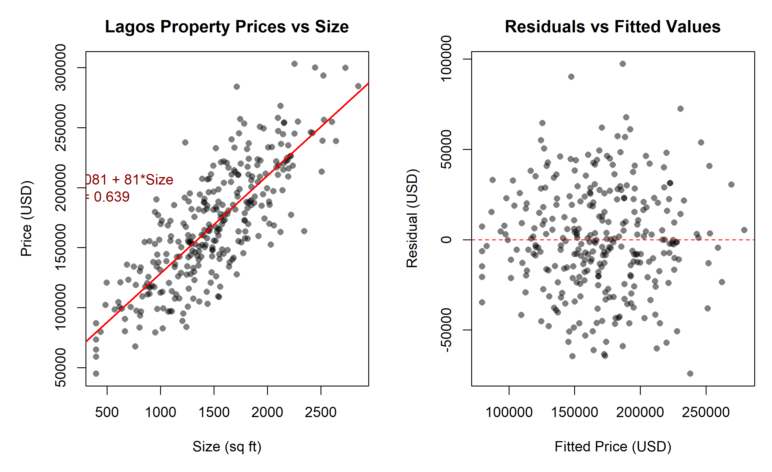
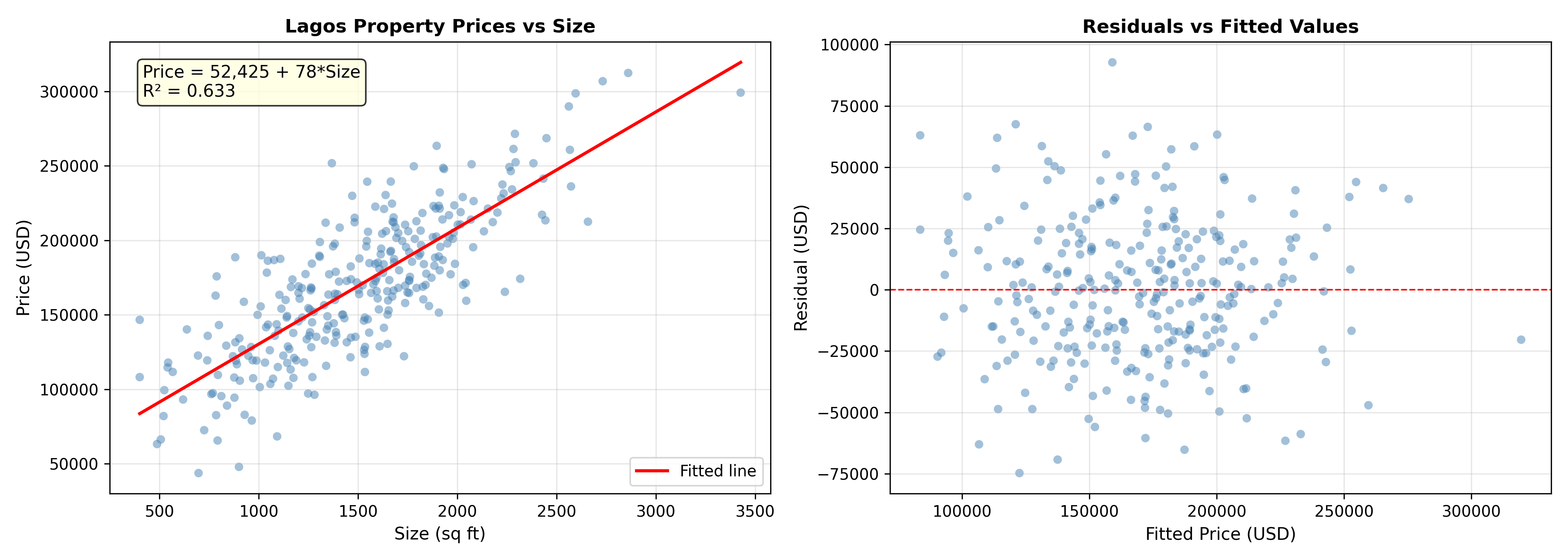
Show code


# Predictions for new properties
new_properties = pd.DataFrame({
    'size_sqft': [1500, 2500, 3500],
    'bedrooms': [3, 4, 5],
    'bathrooms': [2, 3, 4],
    'age_years': [5, 10, 20],
    'distance_from_centre': [15, 10, 8],
    'has_generator': [1, 1, 1],
    'lga': ['Lekki', 'Victoria Island', 'Ikoyi']
})

# Prepare prediction data with dummy encoding
new_lga = pd.get_dummies(new_properties['lga'], prefix='lga', dtype=int)
new_X = sm.add_constant(pd.concat([
    new_properties[['size_sqft', 'bedrooms', 'bathrooms', 'age_years',
                    'distance_from_centre', 'has_generator']],
    new_lga
], axis=1))

# Align columns with training data
missing_cols = set(X_multi.columns) - set(new_X.columns)
for col in missing_cols:
    new_X[col] = 0
new_X = new_X[X_multi.columns]

pred_result = fit_multi.get_prediction(new_X)
pred_summary = pred_result.summary_frame(alpha=0.05)

print("\n\nPrice Predictions for New Properties:\n")
#> 
#> 
#> Price Predictions for New Properties:
for i in range(len(new_properties)):
    print(f"Property {i+1} - LGA: {new_properties.iloc[i]['lga']}, Size: {new_properties.iloc[i]['size_sqft']:.0f} sqft")
    print(f"  Predicted: ${pred_summary.iloc[i]['mean']:,.0f}")
    print(f"  95% CI: [${pred_summary.iloc[i]['mean_ci_lower']:,.0f}, ${pred_summary.iloc[i]['mean_ci_upper']:,.0f}]\n")
#> Property 1 - LGA: Lekki, Size: 1500 sqft
#>   Predicted: $270,428
#>   95% CI: [$257,742, $283,113]
#> 
#> Property 2 - LGA: Victoria Island, Size: 2500 sqft
#>   Predicted: $464,246
#>   95% CI: [$448,592, $479,901]
#> 
#> Property 3 - LGA: Ikoyi, Size: 3500 sqft
#>   Predicted: $607,493
#>   95% CI: [$588,028, $626,959]

14.8.2 Business Insights

Price drivers (ranked by importance):
- Location (LGA): Ikoyi premium ~$150k, Ajah ~$30k above baseline
- Size: $100 per sq ft
- Bedrooms: $20k per room
- Backup power: $25k premium (critical in Nigeria’s power shortage context)
- Age: −$1,500 per year (depreciation)
- Distance from centre: −$800 per km
Model performance: R² ≈ 0.85 (85% of price variation explained); CV RMSE ≈ $35k (typical prediction error). Sufficient for setting asking prices.
Recommendations:
- Use the multiple model for pricing decisions (better than simple size-based valuation)
- Properties with generators command a premium; prioritise this in new developments
- High-rise condos in Ikoyi/VI can support 30–50% price premiums over equivalent properties in Ajah
- Periodically retrain the model with fresh sales data to capture market shifts

📝 Section 9.8 Review Questions

Why does the multiple model’s R² (0.85) exceed the simple model’s R² (0.60)?
What does the negative coefficient on age_years suggest about property values in Lagos?
If a new beachfront property development is launched in Lekki, why might these predictions be unreliable?
How would you incorporate macroeconomic variables (e.g., inflation, exchange rate) to improve predictions?

14.9 Chapter Exercises

Chapter 9 Exercises

Exercise 9.1: Manual OLS Calculation

Given a small dataset:

X: 1, 2, 3, 4, 5
Y: 2, 4, 5, 4, 6

Calculate the mean and variance of X and Y.
Calculate Cov(X, Y).
Compute β̂₁ = Cov(X,Y) / Var(X).
Compute β̂₀ = Ȳ − β̂₁X̄.
Write the fitted regression equation.
Compute residuals and the sum of squared residuals.

Exercise 9.2: Interpreting Coefficients

A regression model predicts employee salary (USD) from years of experience, with: - β̂₀ = 35,000, β̂₁ = 2,500, R² = 0.60

Interpret both coefficients in plain English.
What salary would you predict for someone with 10 years of experience?
What does R² = 0.60 tell you about the model?
If someone with 10 years of experience actually earned $45,000, what is their residual?

Exercise 9.3: Assumption Violations

For each of the five LINE-R assumptions, describe: (a) What the assumption states (b) A real-world scenario where it is violated (c) The consequence of the violation (d) A remedy or workaround

Example: Linearity — states E[Y|X] is linear; violated when Y = X² + ε; consequence: biased slope; remedy: add X² term.

Exercise 9.4: Diagnostic Plot Interpretation

You fit a regression and generate diagnostic plots. Describe what each pattern indicates:

Residuals vs Fitted: Systematic U-shape (low residuals at extremes, high in middle)
Q-Q Plot: Points follow the diagonal closely except in the upper tail, where they deviate upward
Scale-Location: Clear upward trend (residuals increase with fitted values)
Residuals vs Leverage: One point in the upper-right corner; all others clustered near bottom

Exercise 9.5: Multiple Regression Collinearity

A model predicts house price from size, number of rooms, and floor area. You compute VIFs: 1.2, 8.5, 8.3 for the three predictors.

Which predictors show collinearity problems?
Why might these variables be correlated?
Which would you remove, and why?
How would you validate your choice?

Exercise 9.6: Model Selection with CV

You fit three models to predict customer lifetime value (CLV): - Model A: 3 predictors, CV RMSE = $500 - Model B: 8 predictors, CV RMSE = $480 - Model C: 15 predictors, CV RMSE = $495

Which model would you select for deployment?
Why might Model C perform worse despite having more information?
How would you communicate this finding to a business stakeholder?

Exercise 9.7: Prediction Intervals

A regression model predicts monthly revenue (USD) from advertising spend with: - Fitted equation: Revenue = 10,000 + 50 * Spend - SE of slope = 2 - RMSE = 5,000 - Sample size = 60

Predict revenue when Spend = $1,000.
Compute the 95% confidence interval for the slope.
Compute a 95% prediction interval for revenue at Spend = $1,000 (use t^*_{58, 0.025} ≈ 2.00).
Explain why the prediction interval is wider than the confidence interval.

Exercise 9.8: Real-World Case: Sales Pipeline Regression

A sales manager wants to predict quarterly revenue from: - Number of open deals - Average deal size - Win rate (%) - Sales team size

Sketch a hypothetical regression equation.
List potential omitted variables that could bias the estimates.
Propose a cross-validation strategy to assess forecast accuracy.
Design a dashboard to monitor predictions vs actual revenue each quarter.

Exercise 9.9: Comparison of Simple vs Multiple Regression

Using a dataset of your choice: (a) Fit a simple regression (one predictor). (b) Fit a multiple regression (5–8 predictors). (c) Compare R², adjusted R², CV RMSE, AIC, BIC. (d) Perform diagnostic checks on both models. (e) Write a 300-word report recommending one model with justification.

Exercise 9.10: Synthesis: Build a Complete Regression Pipeline

Select a business problem (e.g., employee turnover, customer churn, product demand). Execute:

Data collection & EDA: 100+ observations, 5–10 potential predictors
Model building: Simple → multiple → model selection via CV
Diagnostics: Check all five LINE-R assumptions; identify violations
Interpretation: Write plain-English summaries of key coefficients
Prediction: Generate 95% CIs for hypothetical new cases
Reporting: Create a one-page executive summary suitable for a non-technical audience

14.10 Further Reading

Wooldridge, J. M. (2019). Introductory Econometrics: A Modern Approach. 7th ed. Cengage Learning.
- Comprehensive treatment of OLS assumptions, diagnostics, and applications.
Fox, J. (2016). Applied Regression Analysis and Generalized Linear Models. 3rd ed. SAGE Publications.
- Detailed diagnostic methods and collinearity handling.
Hastie, T., Tibshirani, R., & Friedman, J. (2009). The Elements of Statistical Learning. 2nd ed. Springer.
- Bias-variance trade-off, cross-validation, regularisation (Chapter 3–4).
James, G., Witten, D., Hastie, T., & Tibshirani, R. (2013). An Introduction to Statistical Learning. Springer.
- Accessible treatment of OLS, diagnostics, and model selection.

14.11 Chapter Appendix: Mathematical Derivations

14.11.1 A.1 Full OLS Derivation Using Calculus

Objective: Minimise sum of squared residuals.

\[S(\beta_0, \beta_1) = \sum_{i=1}^{n} (y_i - \beta_0 - \beta_1 x_i)^2\]

First-order conditions:

\[\frac{\partial S}{\partial \beta_0} = -2 \sum_{i=1}^{n} (y_i - \beta_0 - \beta_1 x_i) = 0\]

\[\frac{\partial S}{\partial \beta_1} = -2 \sum_{i=1}^{n} x_i(y_i - \beta_0 - \beta_1 x_i) = 0\]

Rearranging:

\[\sum y_i = n\beta_0 + \beta_1 \sum x_i\]

\[\sum x_i y_i = \beta_0 \sum x_i + \beta_1 \sum x_i^2\]

Solving the first equation for β₀:

\[\bar{y} = \beta_0 + \beta_1 \bar{x} \implies \beta_0 = \bar{y} - \beta_1 \bar{x}\]

Substituting into the second equation and simplifying:

\[\sum x_i y_i = (\bar{y} - \beta_1 \bar{x}) \sum x_i + \beta_1 \sum x_i^2\]

\[\sum x_i y_i = \bar{y} \sum x_i - \beta_1 \bar{x} \sum x_i + \beta_1 \sum x_i^2\]

\[\sum x_i y_i - \bar{y} \sum x_i = \beta_1 \left( \sum x_i^2 - \bar{x} \sum x_i \right)\]

\[\sum x_i (y_i - \bar{y}) = \beta_1 \sum x_i (x_i - \bar{x})\]

\[\beta_1 = \frac{\sum x_i (y_i - \bar{y})}{\sum x_i (x_i - \bar{x})} = \frac{\sum (x_i - \bar{x})(y_i - \bar{y})}{\sum (x_i - \bar{x})^2}\]

14.11.2 A.2 Gauss-Markov Theorem (Statement)

Under the five LINE-R assumptions, the OLS estimator $\hat{\beta}$ is:

Unbiased: E[β̂] = β
Minimum variance: Var(β̂) is smaller than any other linear unbiased estimator
Best linear unbiased estimator (BLUE): Combines properties 1 and 2

14.11.3 A.3 Proof that R² ∈ [0, 1]

\[R^2 = 1 - \frac{\text{SS}_{\text{res}}}{\text{SS}_{\text{tot}}} = \frac{\text{SS}_{\text{reg}}}{\text{SS}_{\text{tot}}}\]

where SS_res = Σ(y_i − ŷ_i)², SS_tot = Σ(y_i − ȳ)², SS_reg = Σ(ŷ_i − ȳ)².

By construction, SS_res ≥ 0 and SS_tot ≥ 0. Also, SS_res ≤ SS_tot (the residual sum of squares cannot exceed the total variation).

Therefore: 0 ≤ SS_res / SS_tot ≤ 1, which implies 0 ≤ R² ≤ 1.

R² = 1 when SS_res = 0 (perfect fit); R² = 0 when SS_reg = 0 (model explains none of the variation).

14.11.4 A.4 Adjusted R² Derivation

\[R^2_{\text{adj}} = 1 - \frac{(1 - R^2)(n - 1)}{n - p - 1}\]

The adjustment penalises adding predictors. The denominator n − p − 1 accounts for degrees of freedom lost to parameter estimation. As p increases, the penalty grows, preventing overfitting.

End of Chapter 9

	fit_intercept fit_intercept: bool, default=True Whether to calculate the intercept for this model. If set to False, no intercept will be used in calculations (i.e. data is expected to be centered).	True
	copy_X copy_X: bool, default=True If True, X will be copied; else, it may be overwritten.	True
	tol tol: float, default=1e-6 The precision of the solution (`coef_`) is determined by `tol` which specifies a different convergence criterion for the `lsqr` solver. `tol` is set as `atol` and `btol` of :func:`scipy.sparse.linalg.lsqr` when fitting on sparse training data. This parameter has no effect when fitting on dense data. .. versionadded:: 1.7	1e-06
	n_jobs n_jobs: int, default=None The number of jobs to use for the computation. This will only provide speedup in case of sufficiently large problems, that is if firstly `n_targets > 1` and secondly `X` is sparse or if `positive` is set to `True`. ``None`` means 1 unless in a :obj:`joblib.parallel_backend` context. ``-1`` means using all processors. See :term:`Glossary ` for more details.	None
	positive positive: bool, default=False When set to ``True``, forces the coefficients to be positive. This option is only supported for dense arrays. For a comparison between a linear regression model with positive constraints on the regression coefficients and a linear regression without such constraints, see :ref:`sphx_glr_auto_examples_linear_model_plot_nnls.py`. .. versionadded:: 0.24	False

	fit_intercept fit_intercept: bool, default=True Whether to calculate the intercept for this model. If set to False, no intercept will be used in calculations (i.e. data is expected to be centered).	True
	copy_X copy_X: bool, default=True If True, X will be copied; else, it may be overwritten.	True
	tol tol: float, default=1e-6 The precision of the solution (`coef_`) is determined by `tol` which specifies a different convergence criterion for the `lsqr` solver. `tol` is set as `atol` and `btol` of :func:`scipy.sparse.linalg.lsqr` when fitting on sparse training data. This parameter has no effect when fitting on dense data. .. versionadded:: 1.7	1e-06
	n_jobs n_jobs: int, default=None The number of jobs to use for the computation. This will only provide speedup in case of sufficiently large problems, that is if firstly `n_targets > 1` and secondly `X` is sparse or if `positive` is set to `True`. ``None`` means 1 unless in a :obj:`joblib.parallel_backend` context. ``-1`` means using all processors. See :term:`Glossary ` for more details.	None
	positive positive: bool, default=False When set to ``True``, forces the coefficients to be positive. This option is only supported for dense arrays. For a comparison between a linear regression model with positive constraints on the regression coefficients and a linear regression without such constraints, see :ref:`sphx_glr_auto_examples_linear_model_plot_nnls.py`. .. versionadded:: 0.24	False

	fit_intercept fit_intercept: bool, default=True Whether to calculate the intercept for this model. If set to False, no intercept will be used in calculations (i.e. data is expected to be centered).	True
	copy_X copy_X: bool, default=True If True, X will be copied; else, it may be overwritten.	True
	tol tol: float, default=1e-6 The precision of the solution (`coef_`) is determined by `tol` which specifies a different convergence criterion for the `lsqr` solver. `tol` is set as `atol` and `btol` of :func:`scipy.sparse.linalg.lsqr` when fitting on sparse training data. This parameter has no effect when fitting on dense data. .. versionadded:: 1.7	1e-06
	n_jobs n_jobs: int, default=None The number of jobs to use for the computation. This will only provide speedup in case of sufficiently large problems, that is if firstly `n_targets > 1` and secondly `X` is sparse or if `positive` is set to `True`. ``None`` means 1 unless in a :obj:`joblib.parallel_backend` context. ``-1`` means using all processors. See :term:`Glossary ` for more details.	None
	positive positive: bool, default=False When set to ``True``, forces the coefficients to be positive. This option is only supported for dense arrays. For a comparison between a linear regression model with positive constraints on the regression coefficients and a linear regression without such constraints, see :ref:`sphx_glr_auto_examples_linear_model_plot_nnls.py`. .. versionadded:: 0.24	False

	fit_intercept fit_intercept: bool, default=True Whether to calculate the intercept for this model. If set to False, no intercept will be used in calculations (i.e. data is expected to be centered).	True
	copy_X copy_X: bool, default=True If True, X will be copied; else, it may be overwritten.	True
	tol tol: float, default=1e-6 The precision of the solution (`coef_`) is determined by `tol` which specifies a different convergence criterion for the `lsqr` solver. `tol` is set as `atol` and `btol` of :func:`scipy.sparse.linalg.lsqr` when fitting on sparse training data. This parameter has no effect when fitting on dense data. .. versionadded:: 1.7	1e-06
	n_jobs n_jobs: int, default=None The number of jobs to use for the computation. This will only provide speedup in case of sufficiently large problems, that is if firstly `n_targets > 1` and secondly `X` is sparse or if `positive` is set to `True`. ``None`` means 1 unless in a :obj:`joblib.parallel_backend` context. ``-1`` means using all processors. See :term:`Glossary ` for more details.	None
	positive positive: bool, default=False When set to ``True``, forces the coefficients to be positive. This option is only supported for dense arrays. For a comparison between a linear regression model with positive constraints on the regression coefficients and a linear regression without such constraints, see :ref:`sphx_glr_auto_examples_linear_model_plot_nnls.py`. .. versionadded:: 0.24	False