---
title: "Fraud Detection"
author: "Bongo Adi"
---

```{python}
#| label: python-setup-36-fraud-detection
#| include: false

import numpy as np
import pandas as pd
import matplotlib.pyplot as plt
import seaborn as sns
import xgboost as xgb
from sklearn.model_selection import train_test_split
from sklearn.preprocessing import StandardScaler
from sklearn.ensemble import IsolationForest
```


::: {.callout-note icon="false"}
## 📋 Learning Objectives

- Understand the fraud landscape in African fintech and banking, with emphasis on Nigerian context
- Recognise the class imbalance problem and why standard metrics fail for fraud
- Implement rule-based fraud detection systems and their limitations
- Build supervised machine learning models with cost matrices and SMOTE
- Apply unsupervised anomaly detection (Isolation Forest, autoencoders)
- Detect fraud rings using graph-based methods
- Design real-time scoring systems and monitoring pipelines
:::

## The Fraud Landscape

Fraud is endemic in financial systems, especially in developing economies where identity verification, regulatory oversight, and transaction monitoring may be weaker. In Nigeria, the Nigeria Inter-Bank Settlement System (NIBSS) annual fraud reports document billions of Naira in losses. Common fraud types include: (1) **Payment fraud**: Unauthorised card transactions, account compromise, phishing; (2) **Identity theft**: Fraudsters impersonating legitimate customers, using stolen credentials or BVN (Bank Verification Number); (3) **Loan fraud**: False income statements, forged collateral documents, identity misrepresentation; (4) **Money laundering**: Structuring transactions to evade reporting thresholds, using mules and cash-in agents; (5) **SIM swap fraud**: Fraudsters taking over phone numbers to reset passwords and steal mobile money. The financial, reputational, and regulatory costs are substantial. A single data breach exposes a bank to millions in direct losses, regulatory fines (CBN penalties can reach 2% of annual turnover), and loss of customer trust.

The strategic challenge is that fraudsters adapt. A rule that catches a fraud technique today is bypassed tomorrow. Traditional rule-based systems (if transaction amount > ₦500,000 AND unusual_country = TRUE, flag) are rigid and generate many false positives, frustrating customers with legitimate needs. Machine learning models learn patterns of fraud from historical data, but they face an extreme class imbalance: fraud typically comprises 0.1–2% of transactions, sometimes lower in mature markets. A naive classifier that predicts "not fraud" for everything achieves 99% accuracy but misses all frauds. The metric that matters in fraud is **precision-recall** (or equivalently, F1 score and lift), not overall accuracy.

## The Class Imbalance Problem Revisited

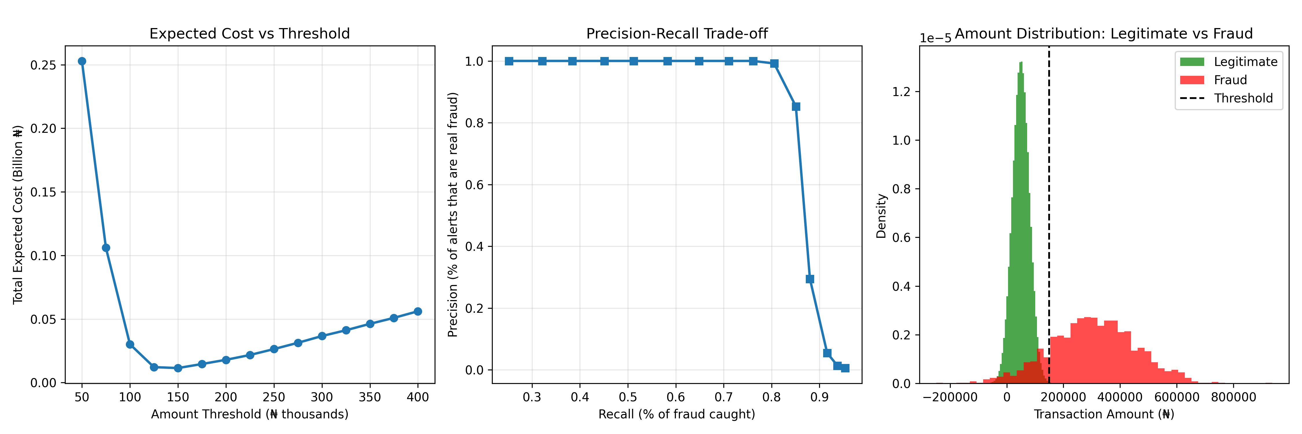
Class imbalance is the core challenge in fraud detection. Given a dataset with 99.5% legitimate transactions and 0.5% fraud, a model that always predicts "legitimate" has 99.5% accuracy but fails utterly. Standard metrics (accuracy, ROC-AUC in extreme imbalance) become misleading. Instead, practitioners use precision, recall, and F1-score. **Precision** = (Fraud caught) / (Total flagged) answers: "Of the alerts we send, how many are real fraud?" **Recall** = (Fraud caught) / (All fraud) answers: "Of the fraud that happened, what fraction did we catch?" There is a trade-off: stricter rules catch more fraud (high recall) but flag many innocents (low precision).

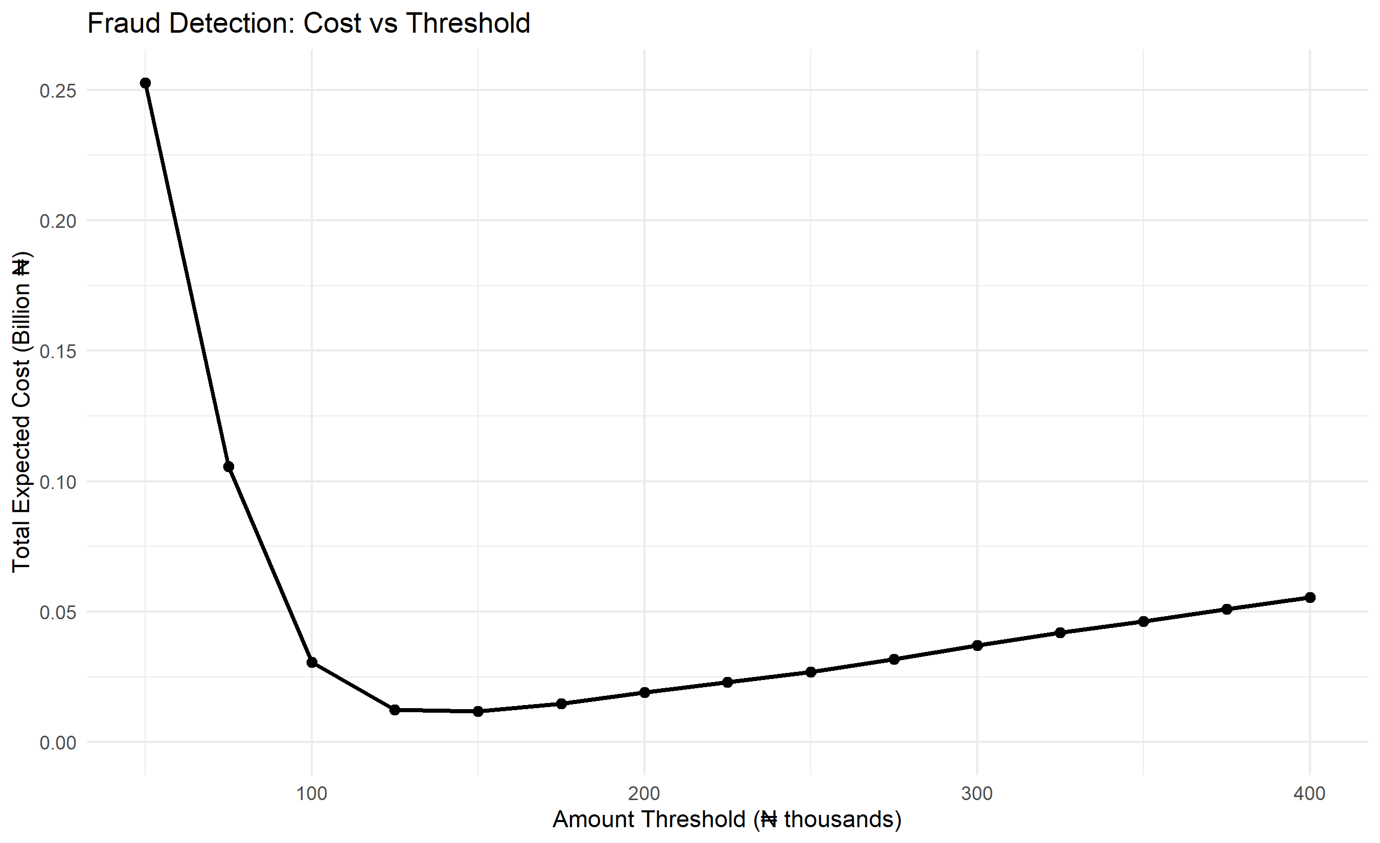
The **cost matrix** formalises this trade-off. A false positive (flagging a legitimate transaction) costs ₦1,000 in customer friction and operational overhead. A false negative (missing fraud) costs ₦50,000 in direct losses, chargebacks, and regulatory provisions. So catching 100 frauds at the cost of 1,000 false positives is a profitable trade. The optimal threshold is not 0.5; it is wherever the expected cost is minimised: $\text{Cost} = (1 - \text{Recall}) \times \text{Fraud}\_\text{Cost} + (1 - \text{Precision}) \times \text{FP}\_\text{Cost}$. Methods like SMOTE (Synthetic Minority Over-sampling Technique) artificially generate synthetic fraud samples to balance classes, allowing standard algorithms to work better. Weighted loss functions apply higher penalty to misclassifying fraud.

::: {.callout-note icon="false"}
## 📘 Theory: Class Imbalance and Cost-Sensitive Learning
:::

::: {.callout-tip icon="false"}
## 🔑 Key Formula

**Precision and Recall (for fraud):**
$$\text{Precision} = \frac{TP}{TP + FP}, \quad \text{Recall} = \frac{TP}{TP + FN}$$

**F1 Score (harmonic mean):**
$$F_1 = 2 \times \frac{\text{Precision} \times \text{Recall}}{\text{Precision} + \text{Recall}}$$

**Cost-Weighted Classification:**
$$\text{Optimal Threshold} = \arg\min_\theta \left[ (1-R(\theta)) \times C_{\text{FN}} + (1-P(\theta)) \times C_{\text{FP}} \right]$$

where $C_{\text{FN}}$ and $C_{\text{FP}}$ are the costs of missing fraud and false positives.
:::

::: {.panel-tabset}
## R
```{r}
#| label: imbalance-problem
# Demonstrate the class imbalance problem in fraud detection

set.seed(4738)

# Generate synthetic NIBSS-style transaction data
n_transactions <- 500000
fraud_rate <- 0.003  # 0.3% fraud
n_fraud <- as.integer(n_transactions * fraud_rate)
n_legitimate <- n_transactions - n_fraud

# Legitimate transactions: smaller amounts, regular patterns
legitimate_amount <- rnorm(n_legitimate, mean = 50000, sd = 30000)
legitimate_transactions <- data.frame(
  amount = legitimate_amount,
  is_fraud = 0
)

# Fraud transactions: tend to be larger, at unusual times
fraud_amount <- rnorm(n_fraud, mean = 300000, sd = 150000)
fraud_transactions <- data.frame(
  amount = fraud_amount,
  is_fraud = 1
)

# Combine
transactions <- rbind(legitimate_transactions, fraud_transactions)

cat("=== Class Imbalance Problem in Fraud Detection ===\n\n")
cat("Dataset:\n")
cat("Total transactions:", nrow(transactions), "\n")
cat("Legitimate transactions:", sum(transactions$is_fraud == 0), "(",
    round(100 * mean(transactions$is_fraud == 0), 2), "%)\n")
cat("Fraud transactions:", sum(transactions$is_fraud == 1), "(",
    round(100 * mean(transactions$is_fraud == 1), 2), "%)\n\n")

# Naive classifier: always predict "legitimate"
naive_accuracy <- mean(transactions$is_fraud == 0)

cat("Naive Classifier (always predicts 'Not Fraud'):\n")
cat("Accuracy:", round(naive_accuracy, 4), "\n")
cat("Recall (catches fraud):", 0, "\n")
cat("Precision:", "Undefined (no positive predictions)\n")
cat("Usefulness: USELESS (misses all fraud)\n\n")

# A better classifier: threshold-based on amount
threshold <- 150000
predicted_fraud <- as.numeric(transactions$amount > threshold)

accuracy <- mean(predicted_fraud == transactions$is_fraud)
precision <- sum(predicted_fraud == 1 & transactions$is_fraud == 1) / sum(predicted_fraud == 1)
recall <- sum(predicted_fraud == 1 & transactions$is_fraud == 1) / sum(transactions$is_fraud == 1)
f1 <- 2 * precision * recall / (precision + recall)

cat("Amount > ₦150,000 Rule:\n")
cat("Accuracy:", round(accuracy, 4), "\n")
cat("Precision:", round(precision, 4), "->", round(100 * precision, 2), "% of flagged are actual fraud\n")
cat("Recall:", round(recall, 4), "->", round(100 * recall, 2), "% of fraud caught\n")
cat("F1-Score:", round(f1, 4), "\n\n")

# Cost matrix: FN costs ₦50,000, FP costs ₦1,000
cost_fn <- 50000
cost_fp <- 1000

# Calculate expected cost for different thresholds
thresholds <- seq(50000, 400000, by = 25000)
costs <- numeric(length(thresholds))
recalls <- numeric(length(thresholds))
precisions <- numeric(length(thresholds))

for (i in seq_along(thresholds)) {
  pred <- as.numeric(transactions$amount > thresholds[i])
  tp <- sum(pred == 1 & transactions$is_fraud == 1)
  fp <- sum(pred == 1 & transactions$is_fraud == 0)
  fn <- sum(pred == 0 & transactions$is_fraud == 1)

  # Expected cost
  costs[i] <- fn * cost_fn + fp * cost_fp

  precisions[i] <- tp / max(tp + fp, 1)
  recalls[i] <- tp / (tp + fn)
}

# Plot
library(ggplot2)

cost_df <- data.frame(
  threshold = thresholds,
  total_cost = costs / 1e9,  # Billions of Naira
  recall = recalls,
  precision = precisions
)

ggplot(cost_df, aes(x = threshold / 1000, y = total_cost)) +
  geom_line(linewidth = 1) +
  geom_point(size = 2) +
  theme_minimal() +
  labs(
    title = "Fraud Detection: Cost vs Threshold",
    x = "Amount Threshold (₦ thousands)",
    y = "Total Expected Cost (Billion ₦)"
  ) +
  ylim(0, max(cost_df$total_cost))

# Optimal threshold
optimal_idx <- which.min(costs)
optimal_threshold <- thresholds[optimal_idx]

cat("Optimal Threshold (minimising total cost):", optimal_threshold, "₦\n")
cat("Expected cost:", format(round(costs[optimal_idx]), big.mark = ","), "₦\n")
cat("Recall at optimal:", round(recalls[optimal_idx], 4), "\n")
cat("Precision at optimal:", round(precisions[optimal_idx], 4), "\n")
```

## Python
```{python}
#| label: py-imbalance-problem
import numpy as np
import pandas as pd
import matplotlib.pyplot as plt

np.random.seed(4738)

# Generate NIBSS-style transaction data
n_transactions = 500000
fraud_rate = 0.003
n_fraud = int(n_transactions * fraud_rate)
n_legitimate = n_transactions - n_fraud

# Legitimate transactions
legit_amount = np.random.normal(50000, 30000, n_legitimate)
legit_df = pd.DataFrame({'amount': legit_amount, 'is_fraud': 0})

# Fraud transactions (larger amounts)
fraud_amount = np.random.normal(300000, 150000, n_fraud)
fraud_df = pd.DataFrame({'amount': fraud_amount, 'is_fraud': 1})

transactions = pd.concat([legit_df, fraud_df], ignore_index=True)

print("=== Class Imbalance Problem in Fraud Detection ===\n")
print("Dataset:")
print(f"Total transactions: {len(transactions)}")
print(f"Legitimate: {(transactions['is_fraud'] == 0).sum()} ({100*(transactions['is_fraud']==0).mean():.2f}%)")
print(f"Fraud: {(transactions['is_fraud'] == 1).sum()} ({100*(transactions['is_fraud']==1).mean():.2f}%)\n")

# Naive classifier
naive_accuracy = (transactions['is_fraud'] == 0).mean()
print("Naive Classifier (always 'Not Fraud'):")
print(f"Accuracy: {naive_accuracy:.4f}")
print(f"Recall: 0 (catches 0% of fraud)")
print(f"Usefulness: USELESS\n")

# Amount threshold rule
def evaluate_threshold(data, threshold):
    pred = (data['amount'] > threshold).astype(int)
    tp = ((pred == 1) & (data['is_fraud'] == 1)).sum()
    fp = ((pred == 1) & (data['is_fraud'] == 0)).sum()
    fn = ((pred == 0) & (data['is_fraud'] == 1)).sum()

    precision = tp / (tp + fp) if (tp + fp) > 0 else 0
    recall = tp / (tp + fn) if (tp + fn) > 0 else 0
    f1 = 2 * precision * recall / (precision + recall) if (precision + recall) > 0 else 0

    return precision, recall, f1, tp, fp, fn

threshold = 150000
precision, recall, f1, tp, fp, fn = evaluate_threshold(transactions, threshold)

print(f"Amount > ₦{threshold} Rule:")
print(f"Precision: {precision:.4f} ({100*precision:.2f}% of flagged are fraud)")
print(f"Recall: {recall:.4f} ({100*recall:.2f}% of fraud caught)")
print(f"F1-Score: {f1:.4f}\n")

# Cost analysis
cost_fn = 50000
cost_fp = 1000

thresholds = np.linspace(50000, 400000, 15)
costs = []
recalls_list = []
precisions_list = []

for t in thresholds:
    prec, rec, _, tp, fp, fn = evaluate_threshold(transactions, t)
    cost = fn * cost_fn + fp * cost_fp
    costs.append(cost)
    recalls_list.append(rec)
    precisions_list.append(prec)

# Plot
fig, axes = plt.subplots(1, 3, figsize=(15, 5))

# Cost vs threshold
axes[0].plot(thresholds/1000, np.array(costs)/1e9, marker='o', linewidth=2)
axes[0].set_xlabel('Amount Threshold (₦ thousands)')
axes[0].set_ylabel('Total Expected Cost (Billion ₦)')
axes[0].set_title('Expected Cost vs Threshold')
axes[0].grid(True, alpha=0.3)

# Precision-recall trade-off
axes[1].plot(recalls_list, precisions_list, marker='s', linewidth=2)
axes[1].set_xlabel('Recall (% of fraud caught)')
axes[1].set_ylabel('Precision (% of alerts that are real fraud)')
axes[1].set_title('Precision-Recall Trade-off')
axes[1].grid(True, alpha=0.3)

# Amount distributions
axes[2].hist(legit_df['amount'], bins=50, alpha=0.7, label='Legitimate', color='green', density=True)
axes[2].hist(fraud_df['amount'], bins=50, alpha=0.7, label='Fraud', color='red', density=True)
axes[2].axvline(x=150000, color='black', linestyle='--', label='Threshold')
axes[2].set_xlabel('Transaction Amount (₦)')
axes[2].set_ylabel('Density')
axes[2].set_title('Amount Distribution: Legitimate vs Fraud')
axes[2].legend()

plt.tight_layout()
plt.show()

# Optimal threshold
optimal_idx = np.argmin(costs)
optimal_threshold = thresholds[optimal_idx]
print(f"Optimal Threshold (min cost): ₦{optimal_threshold:,.0f}")
print(f"Expected cost: ₦{costs[optimal_idx]:,.0f}")
print(f"Recall: {recalls_list[optimal_idx]:.4f}, Precision: {precisions_list[optimal_idx]:.4f}")
```
:::

::: {.callout-caution icon="false"}
## 📝 Section 36.2 Review Questions

1. Why is accuracy misleading as a metric for fraud detection?
2. What is the precision-recall trade-off, and how do we choose the optimal balance?
3. How would you estimate the cost of a false positive and false negative in fraud?
4. What is SMOTE, and how does it help with imbalanced datasets?
:::

## Rule-Based Systems

Historically, fraud detection relied entirely on rules. An expert (domain specialist) observes fraud patterns and translates them into Boolean logic: if condition_1 AND condition_2 AND condition_3, flag as suspicious. Examples:

- If amount > ₦1,000,000 AND unusual_country = TRUE AND new_card, flag.
- If velocity (transactions per hour) > 10, flag.
- If distance_from_home > 1,000 km AND amount > median, flag.

Rules are transparent, explainable, and immediately actionable by analysts. A transaction flagged by a clear rule can be quickly reviewed. They also have zero false negatives for **known patterns**: if the rule perfectly captures a fraud technique, all such frauds are caught. However, rules are brittle. Fraudsters observe rules and adapt. If the rule is "unusual_country = TRUE," fraudsters stop using foreign cards, starting instead to test stolen cards domestically. Rules also generate many false positives, overwhelming analysts. A typical bank's rule set may flag 10,000 transactions a day as suspicious, requiring a team of 50+ analysts to review them.

A modern approach combines rules and machine learning: rules handle obvious, known patterns; machine learning flags suspicious patterns not captured by rules. For example, a rule catches velocity fraud; machine learning catches subtle deviations in amount, time-of-day, or merchant patterns.

::: {.callout-note icon="false"}
## 📘 Theory: Rule-Based vs Statistical Fraud Detection
:::

::: {.callout-tip icon="false"}
## 🔑 Key Formula

**Simple Rule:** If $\sum_{i=1}^{k} \mathbb{1}[\text{Condition}_i] \geq m$, flag as fraud.

**Weighted Rule:** If $\sum_{i=1}^{k} w_i \times \mathbb{1}[\text{Condition}_i] \geq \text{threshold}$, flag.

**Velocity Rule:** If $\frac{\text{# transactions in past hour}}{\text{typical daily rate}} > 10$, flag.
:::

::: {.panel-tabset}
## R
```{r}
#| label: rule-based-fraud
# Rule-based fraud detection system

set.seed(8527)

# Generate synthetic transaction data with multiple features
n_trans <- 50000
data <- data.frame(
  tx_id = 1:n_trans,
  amount = rnorm(n_trans, mean = 50000, sd = 40000),
  is_new_card = sample(c(0, 1), n_trans, replace = TRUE, prob = c(0.95, 0.05)),
  is_foreign_merchant = sample(c(0, 1), n_trans, replace = TRUE, prob = c(0.98, 0.02)),
  is_unusual_time = sample(c(0, 1), n_trans, replace = TRUE, prob = c(0.95, 0.05)),
  is_high_velocity = sample(c(0, 1), n_trans, replace = TRUE, prob = c(0.99, 0.01)),
  is_distance_far = sample(c(0, 1), n_trans, replace = TRUE, prob = c(0.96, 0.04))
)

# True fraud: happens in combinations
# Fraud rule: (new_card OR foreign_merchant) AND (high_velocity OR unusual_time)
# Plus some random fraud
fraud_prob <- (
  ((data$is_new_card + data$is_foreign_merchant > 0) &
   (data$is_high_velocity + data$is_unusual_time > 0)) * 0.3 +
  (data$is_distance_far * 0.1) +
  0.003  # Base fraud rate
)
fraud_prob <- pmin(fraud_prob, 1)
data$is_fraud <- as.numeric(runif(n_trans) < fraud_prob)

cat("=== Rule-Based Fraud Detection System ===\n\n")

# Rule 1: Amount
rule1 <- data$amount > 300000
cat("Rule 1 (Amount > ₦300,000):\n")
cat("  Flagged:", sum(rule1), "transactions\n")
cat("  Fraud caught:", sum(rule1 & data$is_fraud), "\n")
cat("  Precision:", round(sum(rule1 & data$is_fraud) / sum(rule1), 4), "\n\n")

# Rule 2: Velocity
rule2 <- data$is_high_velocity == 1
cat("Rule 2 (High velocity):\n")
cat("  Flagged:", sum(rule2), "\n")
cat("  Fraud caught:", sum(rule2 & data$is_fraud), "\n")
cat("  Precision:", round(sum(rule2 & data$is_fraud) / sum(rule2), 4), "\n\n")

# Rule 3: New card + foreign merchant
rule3 <- (data$is_new_card == 1) & (data$is_foreign_merchant == 1)
cat("Rule 3 (New card + Foreign merchant):\n")
cat("  Flagged:", sum(rule3), "\n")
cat("  Fraud caught:", sum(rule3 & data$is_fraud), "\n")
cat("  Precision:", round(sum(rule3 & data$is_fraud) / sum(rule3), 4), "\n\n")

# Combined rule (OR: flag if ANY rule triggers)
combined_or <- rule1 | rule2 | rule3
cat("Combined Rule (OR logic - flag if ANY rule):\n")
cat("  Flagged:", sum(combined_or), "\n")
cat("  Fraud caught:", sum(combined_or & data$is_fraud), "\n")
cat("  Recall:", round(sum(combined_or & data$is_fraud) / sum(data$is_fraud), 4), "\n")
cat("  Precision:", round(sum(combined_or & data$is_fraud) / sum(combined_or), 4), "\n")
cat("  False positives:", sum(combined_or & data$is_fraud == 0), "\n\n")

# Weighted rule
weighted_score <- (
  rule1 * 20 +  # High suspicion
  rule2 * 30 +
  rule3 * 25 +
  (data$is_unusual_time == 1) * 10 +
  (data$is_distance_far == 1) * 15
)

threshold <- 30
weighted_flag <- weighted_score >= threshold

cat("Weighted Rule (score >= 30):\n")
cat("  Flagged:", sum(weighted_flag), "\n")
cat("  Fraud caught:", sum(weighted_flag & data$is_fraud), "\n")
cat("  Recall:", round(sum(weighted_flag & data$is_fraud) / sum(data$is_fraud), 4), "\n")
cat("  Precision:", round(sum(weighted_flag & data$is_fraud) / sum(weighted_flag), 4), "\n")
cat("  False positives:", sum(weighted_flag & data$is_fraud == 0), "\n")
```

## Python
```{python}
#| label: py-rule-based-fraud
import numpy as np
import pandas as pd

np.random.seed(8527)

# Generate transaction data
n_trans = 50000
data = pd.DataFrame({
    'tx_id': range(1, n_trans + 1),
    'amount': np.random.normal(50000, 40000, n_trans),
    'is_new_card': np.random.choice([0, 1], n_trans, p=[0.95, 0.05]),
    'is_foreign_merchant': np.random.choice([0, 1], n_trans, p=[0.98, 0.02]),
    'is_unusual_time': np.random.choice([0, 1], n_trans, p=[0.95, 0.05]),
    'is_high_velocity': np.random.choice([0, 1], n_trans, p=[0.99, 0.01]),
    'is_distance_far': np.random.choice([0, 1], n_trans, p=[0.96, 0.04])
})

# True fraud patterns
fraud_prob = (
    ((data['is_new_card'] + data['is_foreign_merchant'] > 0) &
     (data['is_high_velocity'] + data['is_unusual_time'] > 0)) * 0.3 +
    (data['is_distance_far'] * 0.1) +
    0.003
)
fraud_prob = np.clip(fraud_prob, 0, 1)
data['is_fraud'] = (np.random.rand(n_trans) < fraud_prob).astype(int)

print("=== Rule-Based Fraud Detection System ===\n")

# Rule 1: Amount
rule1 = data['amount'] > 300000
print("Rule 1 (Amount > ₦300,000):")
print(f"  Flagged: {rule1.sum()}")
print(f"  Fraud caught: {(rule1 & (data['is_fraud'] == 1)).sum()}")
precision1 = (rule1 & (data['is_fraud'] == 1)).sum() / rule1.sum()
print(f"  Precision: {precision1:.4f}\n")

# Rule 2: Velocity
rule2 = data['is_high_velocity'] == 1
print("Rule 2 (High velocity):")
print(f"  Flagged: {rule2.sum()}")
print(f"  Fraud caught: {(rule2 & (data['is_fraud'] == 1)).sum()}")
precision2 = (rule2 & (data['is_fraud'] == 1)).sum() / rule2.sum() if rule2.sum() > 0 else 0
print(f"  Precision: {precision2:.4f}\n")

# Rule 3: New card + foreign merchant
rule3 = (data['is_new_card'] == 1) & (data['is_foreign_merchant'] == 1)
print("Rule 3 (New card + Foreign merchant):")
print(f"  Flagged: {rule3.sum()}")
print(f"  Fraud caught: {(rule3 & (data['is_fraud'] == 1)).sum()}")
precision3 = (rule3 & (data['is_fraud'] == 1)).sum() / rule3.sum() if rule3.sum() > 0 else 0
print(f"  Precision: {precision3:.4f}\n")

# Combined OR
combined = rule1 | rule2 | rule3
fraud_caught = (combined & (data['is_fraud'] == 1)).sum()
recall = fraud_caught / (data['is_fraud'] == 1).sum()
precision = fraud_caught / combined.sum() if combined.sum() > 0 else 0
print(f"Combined Rule (OR - flag if ANY):")
print(f"  Flagged: {combined.sum()}")
print(f"  Fraud caught: {fraud_caught}")
print(f"  Recall: {recall:.4f}, Precision: {precision:.4f}")
print(f"  False positives: {(combined & (data['is_fraud'] == 0)).sum()}\n")

# Weighted rule
weighted_score = (
    rule1.astype(int) * 20 +
    rule2.astype(int) * 30 +
    rule3.astype(int) * 25 +
    (data['is_unusual_time'] * 10) +
    (data['is_distance_far'] * 15)
)

weighted_flag = weighted_score >= 30
fraud_caught_w = (weighted_flag & (data['is_fraud'] == 1)).sum()
recall_w = fraud_caught_w / (data['is_fraud'] == 1).sum()
precision_w = fraud_caught_w / weighted_flag.sum() if weighted_flag.sum() > 0 else 0

print(f"Weighted Rule (score >= 30):")
print(f"  Flagged: {weighted_flag.sum()}")
print(f"  Fraud caught: {fraud_caught_w}")
print(f"  Recall: {recall_w:.4f}, Precision: {precision_w:.4f}")
print(f"  False positives: {(weighted_flag & (data['is_fraud'] == 0)).sum()}")
```
:::

::: {.callout-caution icon="false"}
## 📝 Section 36.3 Review Questions

1. What is the advantage of rule-based fraud detection? What is the disadvantage?
2. How would you design a weighted rule system that balances coverage and precision?
3. Why might rules generate high false positives?
4. How would you adapt a rule system if fraudsters learn to evade it?
:::

## Supervised Fraud Models

Machine learning models trained on historical fraud data can capture patterns more flexibly than hand-coded rules. The challenge is handling the class imbalance. Standard logistic regression or decision trees, trained on 99.5% non-fraud data, learn that "non-fraud" is the safe default; they rarely predict fraud even when features suggest it.

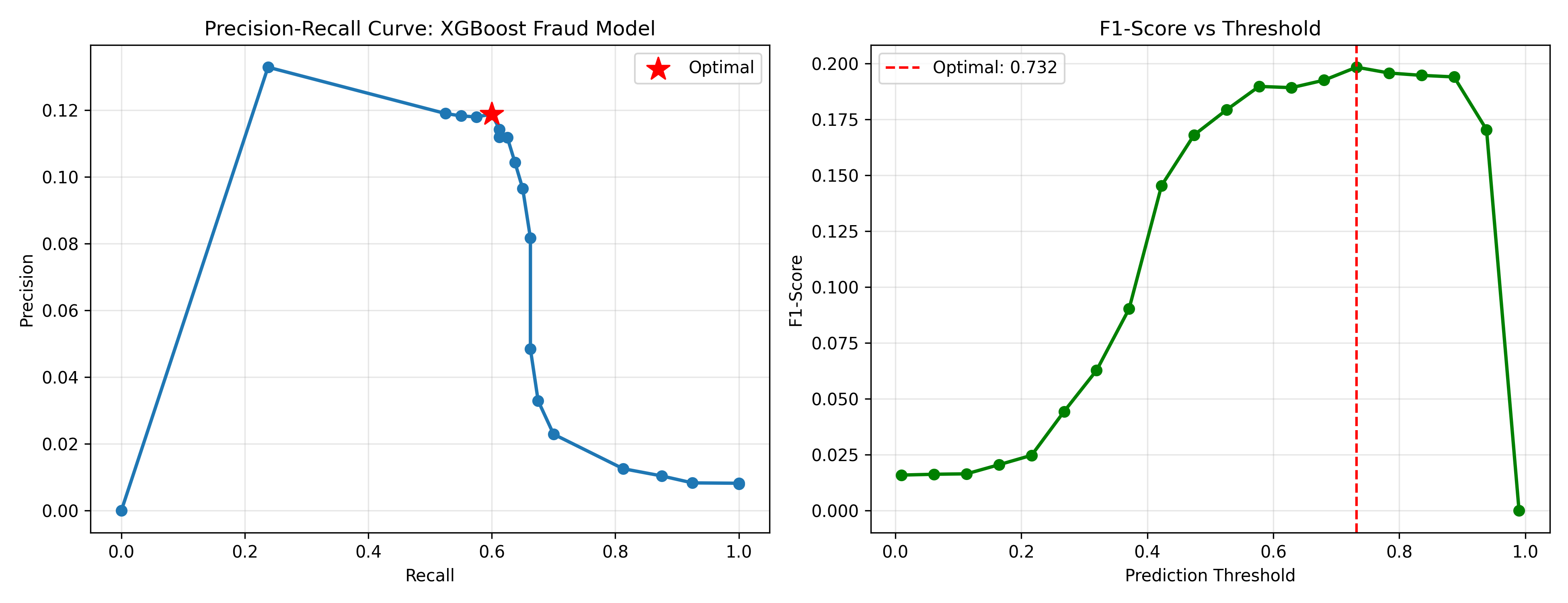
Solutions include: (1) **Class weighting**: Penalise fraud misclassification (false negatives) more heavily in the loss function. A penalty ratio of 200:1 (cost of missing fraud : cost of false alarm) is common. (2) **SMOTE (Synthetic Minority Over-sampling Technique)**: Generate synthetic fraud samples using nearest neighbours in feature space. If a real fraud has features $\mathbf{x}_1$ and its nearest neighbour (also fraud) has $\mathbf{x}_2$, create a synthetic sample at $\mathbf{x}_1 + \alpha(\mathbf{x}_2 - \mathbf{x}_1)$ for random $\alpha \in [0,1]$. This inflates the fraud class without duplicating exactly. (3) **Threshold tuning**: Train on balanced or weighted data, then adjust the decision threshold post-hoc to maximise F1 score or a business metric (expected cost).

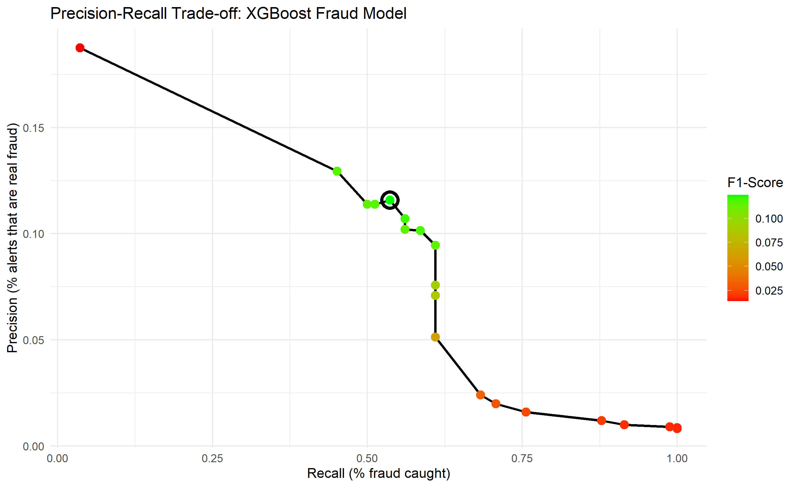
XGBoost handles class weighting well via the `scale_pos_weight` parameter. After training, we don't use threshold 0.5; we choose a threshold that maximises expected profit given the cost matrix.

::: {.callout-note icon="false"}
## 📘 Theory: Class Balancing for Fraud
:::

::: {.callout-tip icon="false"}
## 🔑 Key Formula

**SMOTE: Generate Synthetic Minority Samples**
$$\mathbf{x}_{\text{synthetic}} = \mathbf{x}_i + \lambda (\mathbf{x}_{k-\text{NN}} - \mathbf{x}_i), \quad \lambda \sim U(0, 1)$$

**Weighted Loss for Class Imbalance:**
$$L = w_0 \sum_{i: y_i = 0} \ell(y_i, \hat{y}_i) + w_1 \sum_{i: y_i = 1} \ell(y_i, \hat{y}_i)$$

Typical: $w_1 / w_0 = (\text{# Negatives}) / (\text{# Positives})$.

**XGBoost scale_pos_weight:**
$$\text{scale\_pos\_weight} = w_1 / w_0$$
:::

::: {.panel-tabset}
## R
```{r}
#| label: supervised-fraud-models
# Supervised models for fraud detection with class balancing

library(xgboost)
library(caret)

# Use the synthetic fraud data from earlier
set.seed(6384)

# Prepare features
features <- c("amount", "is_new_card", "is_foreign_merchant",
              "is_unusual_time", "is_high_velocity", "is_distance_far")
X <- as.matrix(data[, features])

# Standardize
X <- scale(X)

y <- data$is_fraud

# Train-test split
train_idx <- createDataPartition(y, p = 0.8, list = FALSE)
X_train <- X[train_idx, ]
y_train <- y[train_idx]
X_test <- X[-train_idx, ]
y_test <- y[-train_idx]

cat("=== Supervised Fraud Detection ===\n\n")
cat("Training set fraud rate:", round(mean(y_train), 4), "\n")
cat("Test set fraud rate:", round(mean(y_test), 4), "\n\n")

# XGBoost with class weighting
scale_pos_weight <- sum(y_train == 0) / sum(y_train == 1)

dtrain <- xgb.DMatrix(data = X_train, label = y_train)
dtest <- xgb.DMatrix(data = X_test, label = y_test)

params <- list(
  objective = "binary:logistic",
  scale_pos_weight = scale_pos_weight,
  max_depth = 4,
  eta = 0.1,
  min_child_weight = 1
)

xgb_model <- xgb.train(
  params = params,
  data = dtrain,
  nrounds = 100,
  watchlist = list(test = dtest),
  verbose = 0
)

# Predictions
y_pred <- predict(xgb_model, dtest)

# Evaluate at different thresholds
thresholds <- seq(0.01, 0.99, by = 0.05)
results <- data.frame(
  threshold = numeric(),
  recall = numeric(),
  precision = numeric(),
  f1 = numeric(),
  false_positives = numeric()
)

for (i in seq_along(thresholds)) {
  pred <- as.numeric(y_pred > thresholds[i])
  tp <- sum(pred == 1 & y_test == 1)
  fp <- sum(pred == 1 & y_test == 0)
  fn <- sum(pred == 0 & y_test == 1)

  recall <- tp / (tp + fn)
  precision <- tp / max(tp + fp, 1)
  f1 <- 2 * precision * recall / max(precision + recall, 1)

  results <- rbind(results, data.frame(
    threshold = thresholds[i],
    recall = recall,
    precision = precision,
    f1 = f1,
    false_positives = fp
  ))
}

# Find optimal threshold (maximise F1)
optimal_idx <- which.max(results$f1)
optimal_threshold <- results$threshold[optimal_idx]

cat("Optimal Threshold (max F1):", round(optimal_threshold, 3), "\n")
cat("Recall:", round(results$recall[optimal_idx], 4), "\n")
cat("Precision:", round(results$precision[optimal_idx], 4), "\n")
cat("F1-Score:", round(results$f1[optimal_idx], 4), "\n")
cat("False positives:", results$false_positives[optimal_idx], "\n\n")

# Visualize
library(ggplot2)
ggplot(results, aes(x = recall, y = precision)) +
  geom_path(linewidth = 1) +
  geom_point(aes(colour = f1), size = 3) +
  scale_colour_gradient(low = "red", high = "green") +
  theme_minimal() +
  labs(
    title = "Precision-Recall Trade-off: XGBoost Fraud Model",
    x = "Recall (% fraud caught)",
    y = "Precision (% alerts that are real fraud)",
    colour = "F1-Score"
  ) +
  annotate("point", x = results$recall[optimal_idx], y = results$precision[optimal_idx],
           shape = 21, size = 5, color = "black", fill = NA, stroke = 2)
```

## Python
```{python}
#| label: py-supervised-fraud-models
import xgboost as xgb
import numpy as np
import pandas as pd
import matplotlib.pyplot as plt
from sklearn.model_selection import train_test_split
from sklearn.preprocessing import StandardScaler

# Prepare data
features = ['amount', 'is_new_card', 'is_foreign_merchant',
            'is_unusual_time', 'is_high_velocity', 'is_distance_far']
X = data[features].values

# Standardize
scaler = StandardScaler()
X_scaled = scaler.fit_transform(X)

y = data['is_fraud'].values

# Split
X_train, X_test, y_train, y_test = train_test_split(
    X_scaled, y, test_size=0.2, random_state=6384, stratify=y
)

print("=== Supervised Fraud Detection ===\n")
print(f"Training fraud rate: {y_train.mean():.4f}")
print(f"Test fraud rate: {y_test.mean():.4f}\n")

# XGBoost with class weight
scale_pos_weight = (y_train == 0).sum() / (y_train == 1).sum()

dtrain = xgb.DMatrix(X_train, label=y_train)
dtest = xgb.DMatrix(X_test, label=y_test)

params = {
    'objective': 'binary:logistic',
    'scale_pos_weight': scale_pos_weight,
    'max_depth': 4,
    'eta': 0.1,
    'min_child_weight': 1
}

xgb_model = xgb.train(params, dtrain, num_boost_round=100, verbose_eval=False)

# Predictions
y_pred = xgb_model.predict(dtest)

# Evaluate at different thresholds
thresholds = np.linspace(0.01, 0.99, 20)
results = []

for threshold in thresholds:
    pred = (y_pred > threshold).astype(int)
    tp = ((pred == 1) & (y_test == 1)).sum()
    fp = ((pred == 1) & (y_test == 0)).sum()
    fn = ((pred == 0) & (y_test == 1)).sum()

    recall = tp / (tp + fn) if (tp + fn) > 0 else 0
    precision = tp / (tp + fp) if (tp + fp) > 0 else 0
    f1 = 2 * precision * recall / (precision + recall) if (precision + recall) > 0 else 0

    results.append({
        'threshold': threshold,
        'recall': recall,
        'precision': precision,
        'f1': f1,
        'false_positives': fp
    })

results_df = pd.DataFrame(results)
optimal_idx = results_df['f1'].idxmax()
optimal_threshold = results_df.loc[optimal_idx, 'threshold']

print(f"Optimal Threshold (max F1): {optimal_threshold:.3f}")
print(f"Recall: {results_df.loc[optimal_idx, 'recall']:.4f}")
print(f"Precision: {results_df.loc[optimal_idx, 'precision']:.4f}")
print(f"F1-Score: {results_df.loc[optimal_idx, 'f1']:.4f}")
print(f"False positives: {int(results_df.loc[optimal_idx, 'false_positives'])}\n")

# Plot
fig, (ax1, ax2) = plt.subplots(1, 2, figsize=(13, 5))

# Precision-recall curve
ax1.plot(results_df['recall'], results_df['precision'], marker='o', linewidth=2)
ax1.scatter([results_df.loc[optimal_idx, 'recall']], [results_df.loc[optimal_idx, 'precision']],
           s=200, c='red', marker='*', zorder=5, label='Optimal')
ax1.set_xlabel('Recall')
ax1.set_ylabel('Precision')
ax1.set_title('Precision-Recall Curve: XGBoost Fraud Model')
ax1.legend()
ax1.grid(True, alpha=0.3)

# F1 vs threshold
ax2.plot(results_df['threshold'], results_df['f1'], marker='o', linewidth=2, color='green')
ax2.axvline(x=optimal_threshold, color='red', linestyle='--', label=f'Optimal: {optimal_threshold:.3f}')
ax2.set_xlabel('Prediction Threshold')
ax2.set_ylabel('F1-Score')
ax2.set_title('F1-Score vs Threshold')
ax2.legend()
ax2.grid(True, alpha=0.3)

plt.tight_layout()
plt.show()
```
:::

::: {.callout-caution icon="false"}
## 📝 Section 36.4 Review Questions

1. Why is class weighting important in XGBoost for fraud detection?
2. How does SMOTE work, and when should you use it?
3. Why don't we use threshold 0.5 for fraud classification?
4. How would you choose the optimal threshold given a cost matrix?
:::

## Anomaly Detection

Unsupervised anomaly detection finds transactions that deviate significantly from the normal pattern, without requiring historical fraud labels. This is valuable because (a) fraudsters continuously innovate, creating patterns not seen in training data; (b) in new markets, fraud labels may be scarce. Two approaches stand out.

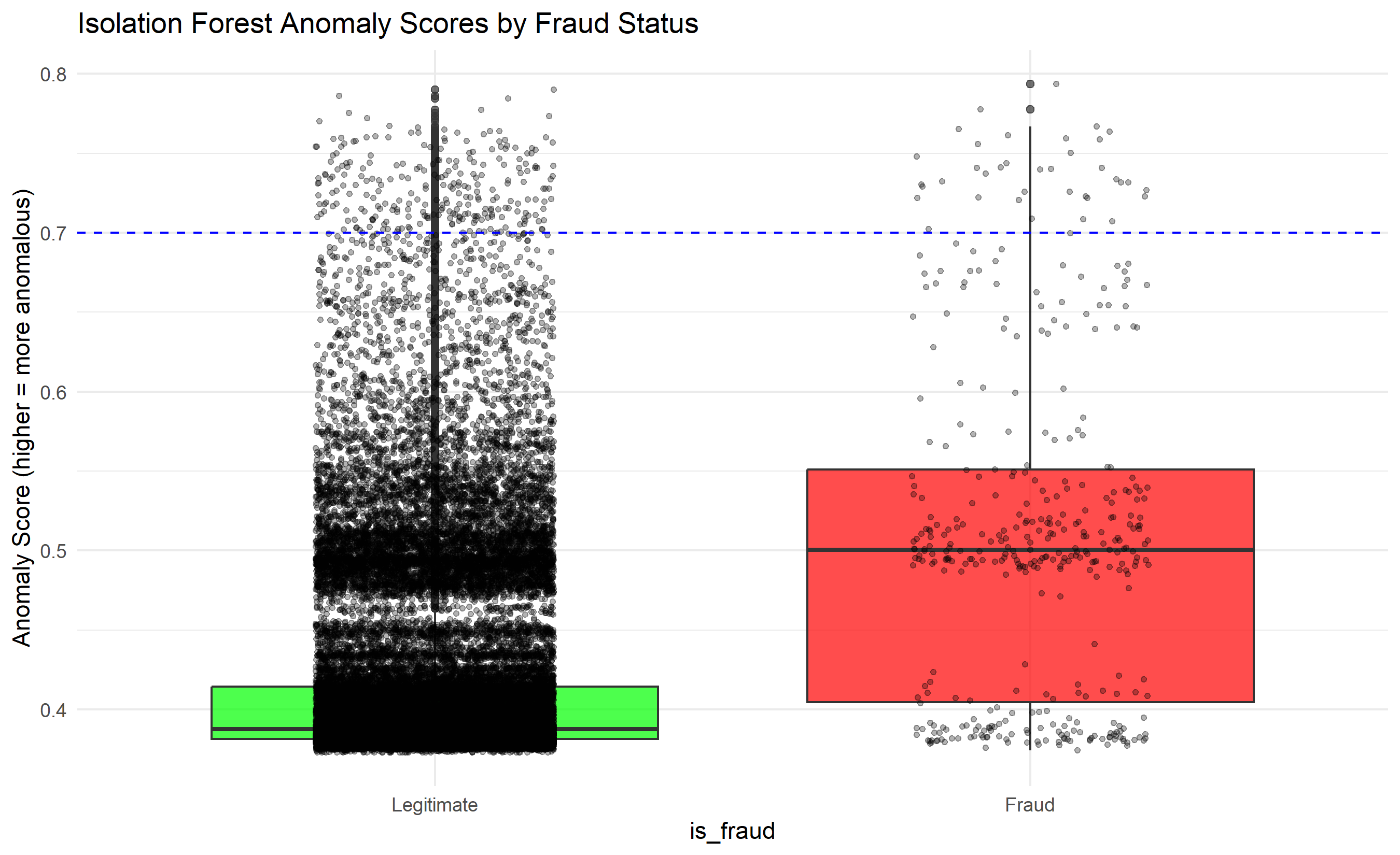
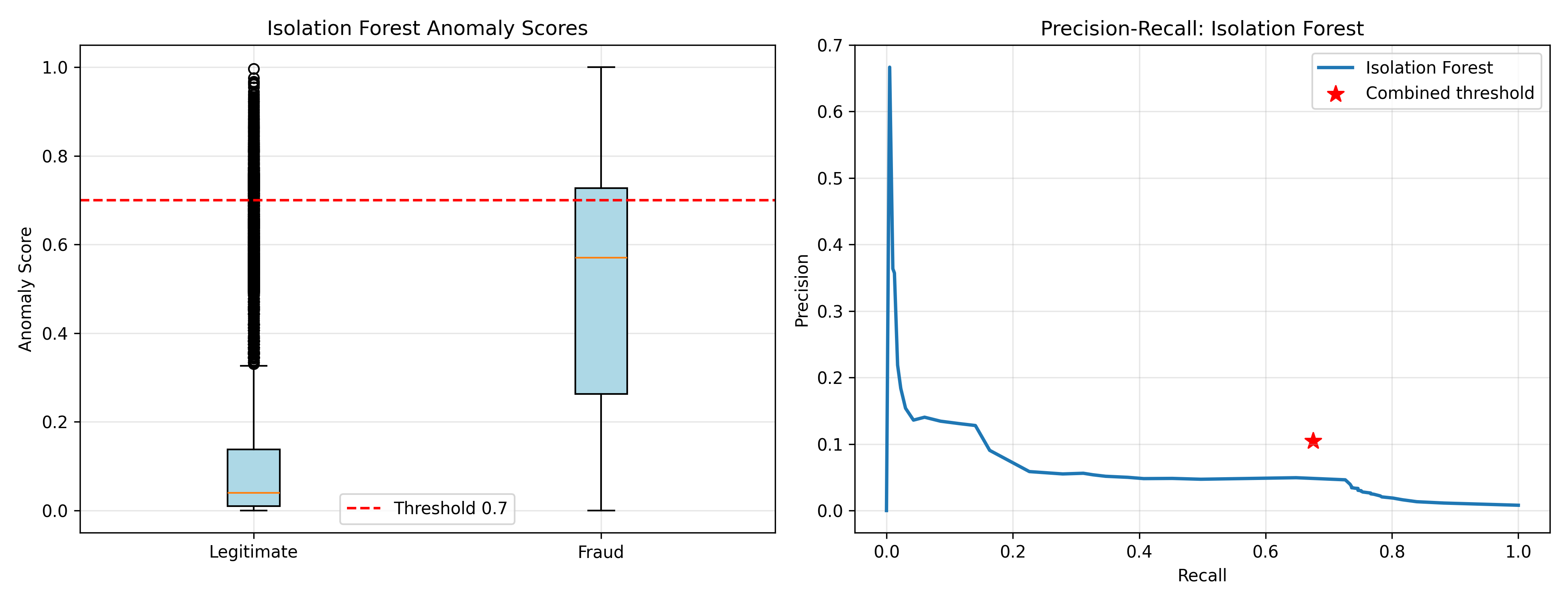
**Isolation Forest** is fast and effective for high-dimensional data. The intuition: anomalies are isolated (few neighbours). Isolation Forest builds random decision trees, splitting on random features and random thresholds. Anomalies require fewer splits to isolate than normal points. Each transaction gets an anomaly score: number of splits needed to isolate it. A score near 0 suggests normal; near 1 suggests anomalous. Isolation Forest is unsupervised (no labels needed), robust to outliers, and fast (O(n log n)).

**Autoencoders** (neural networks) learn to compress and reconstruct normal transactions. A normal transaction (all features of a legitimate purchase) reconstructs well; a fraudulent transaction (unusual feature combinations) has high reconstruction error. Train an autoencoder on only non-fraudulent transactions, then use reconstruction error as the anomaly score. Autoencoders are more flexible than Isolation Forest (can learn complex manifolds) but slower to train.

Both methods complement supervised models. A transaction flagged by both the supervised model and an anomaly detector is very likely fraud.

::: {.callout-note icon="false"}
## 📘 Theory: Unsupervised Anomaly Detection
:::

::: {.callout-tip icon="false"}
## 🔑 Key Formula

**Isolation Forest Anomaly Score:**
$$s(x) = 2^{-E(h(x))/c(n)}$$

where $E(h(x))$ is the expected path length from root to leaf, $c(n)$ is the average path length in isolation trees, and $n$ is sample size.

**Autoencoder Reconstruction Error:**
$$\text{Anomaly Score} = \|\mathbf{x} - \text{Decoder}(\text{Encoder}(\mathbf{x}))\|_2$$

Higher error → more anomalous.
:::

::: {.panel-tabset}
## R
```{r}
#| label: anomaly-detection-fraud
# Anomaly detection for fraud: Isolation Forest

library(isotree)

set.seed(2916)

# Prepare features (excluding fraud label for unsupervised learning)
X_features <- data[, c("amount", "is_new_card", "is_foreign_merchant",
                       "is_unusual_time", "is_high_velocity", "is_distance_far")]
X_scaled <- scale(X_features)

# Train Isolation Forest
iso_model <- isolation.forest(X_scaled, ntrees = 100, nthreads = 1)

# Compute anomaly scores
anomaly_scores <- predict(iso_model, X_scaled)

cat("=== Anomaly Detection: Isolation Forest ===\n\n")
cat("Anomaly score range:", round(min(anomaly_scores), 4), "to", round(max(anomaly_scores), 4), "\n")
cat("Mean anomaly score:", round(mean(anomaly_scores), 4), "\n")
cat("Std dev:", round(sd(anomaly_scores), 4), "\n\n")

# Detect anomalies at different thresholds
anomaly_thresholds <- c(0.6, 0.7, 0.8)

for (threshold in anomaly_thresholds) {
  anomaly_pred <- as.numeric(anomaly_scores > threshold)
  tp <- sum(anomaly_pred == 1 & data$is_fraud == 1)
  fp <- sum(anomaly_pred == 1 & data$is_fraud == 0)
  fn <- sum(anomaly_pred == 0 & data$is_fraud == 1)

  recall <- tp / (tp + fn)
  precision <- tp / max(tp + fp, 1)

  cat(sprintf("Threshold %.2f:\n", threshold))
  cat("  Flagged:", sum(anomaly_pred), "transactions\n")
  cat("  Fraud caught:", tp, "\n")
  cat("  Recall:", round(recall, 4), ", Precision:", round(precision, 4), "\n\n")
}

# Compare to supervised model
# Use predictions from earlier supervised model
supervised_pred <- y_pred

# Combine: flag if EITHER model says anomalous/fraud
combined_pred <- (anomaly_scores > 0.7) | (supervised_pred > 0.5)

cat("Combined (Isolation Forest OR Supervised):\n")
cat("Flagged:", sum(combined_pred), "\n")
tp_combined <- sum(combined_pred & data$is_fraud == 1)
fp_combined <- sum(combined_pred & data$is_fraud == 0)
recall_combined <- tp_combined / sum(data$is_fraud == 1)
precision_combined <- tp_combined / sum(combined_pred)
cat("Fraud caught:", tp_combined, "\n")
cat("Recall:", round(recall_combined, 4), ", Precision:", round(precision_combined, 4), "\n")

# Visualize anomaly scores by true label
library(ggplot2)
score_df <- data.frame(
  anomaly_score = anomaly_scores,
  is_fraud = factor(data$is_fraud, labels = c("Legitimate", "Fraud"))
)

ggplot(score_df, aes(x = is_fraud, y = anomaly_score)) +
  geom_boxplot(fill = c("green", "red"), alpha = 0.7) +
  geom_jitter(width = 0.2, size = 1, alpha = 0.3) +
  theme_minimal() +
  labs(
    title = "Isolation Forest Anomaly Scores by Fraud Status",
    y = "Anomaly Score (higher = more anomalous)"
  ) +
  geom_hline(yintercept = 0.7, linetype = "dashed", colour = "blue", label = "Detection threshold")
```

## Python
```{python}
#| label: py-anomaly-detection-fraud
from sklearn.ensemble import IsolationForest
import numpy as np
import pandas as pd
import matplotlib.pyplot as plt

# Prepare features
features = ['amount', 'is_new_card', 'is_foreign_merchant',
            'is_unusual_time', 'is_high_velocity', 'is_distance_far']
X_features = data[features].values

# Standardize
X_scaled = (X_features - X_features.mean(axis=0)) / (X_features.std(axis=0) + 1e-8)

# Train Isolation Forest
iso_model = IsolationForest(contamination=0.05, random_state=2916, n_estimators=100)
iso_model.fit(X_scaled)

# Anomaly scores (-1 to 1, higher = more anomalous)
anomaly_scores = -iso_model.score_samples(X_scaled)
anomaly_scores = (anomaly_scores - anomaly_scores.min()) / (anomaly_scores.max() - anomaly_scores.min())

print("=== Anomaly Detection: Isolation Forest ===\n")
print(f"Anomaly score range: {anomaly_scores.min():.4f} to {anomaly_scores.max():.4f}")
print(f"Mean: {anomaly_scores.mean():.4f}, Std: {anomaly_scores.std():.4f}\n")

# Evaluate at different thresholds
for threshold in [0.6, 0.7, 0.8]:
    pred = (anomaly_scores > threshold).astype(int)
    tp = ((pred == 1) & (data['is_fraud'] == 1)).sum()
    fp = ((pred == 1) & (data['is_fraud'] == 0)).sum()
    fn = ((pred == 0) & (data['is_fraud'] == 1)).sum()

    recall = tp / (tp + fn) if (tp + fn) > 0 else 0
    precision = tp / (tp + fp) if (tp + fp) > 0 else 0

    print(f"Threshold {threshold:.2f}:")
    print(f"  Flagged: {pred.sum()} transactions")
    print(f"  Fraud caught: {tp}")
    print(f"  Recall: {recall:.4f}, Precision: {precision:.4f}\n")

# Combined with supervised — re-score the same test set used by XGBoost
# X_test comes from the supervised block (StandardScaler, same 6 features)
anon_test = -iso_model.score_samples(X_test)
anon_test_norm = (anon_test - anomaly_scores.min()) / (anomaly_scores.max() - anomaly_scores.min())
combined = (anon_test_norm > 0.7) | (y_pred > 0.5)
tp_combined = ((combined) & (y_test == 1)).sum()
fp_combined = ((combined) & (y_test == 0)).sum()
recall_combined = tp_combined / (y_test == 1).sum()
precision_combined = tp_combined / combined.sum() if combined.sum() > 0 else 0

print("Combined (IF OR Supervised):")
print(f"  Flagged: {combined.sum()}")
print(f"  Fraud caught: {tp_combined}")
print(f"  Recall: {recall_combined:.4f}, Precision: {precision_combined:.4f}\n")

# Visualize
fig, (ax1, ax2) = plt.subplots(1, 2, figsize=(13, 5))

# Box plot of anomaly scores
legitimate_scores = anomaly_scores[data['is_fraud'] == 0]
fraud_scores = anomaly_scores[data['is_fraud'] == 1]

ax1.boxplot([legitimate_scores, fraud_scores], labels=['Legitimate', 'Fraud'],
           patch_artist=True, boxprops=dict(facecolor='lightblue'))
ax1.axhline(y=0.7, color='red', linestyle='--', label='Threshold 0.7')
ax1.set_ylabel('Anomaly Score')
ax1.set_title('Isolation Forest Anomaly Scores')
ax1.legend()
ax1.grid(True, alpha=0.3)

# ROC-like curve
thresholds = np.linspace(0, 1, 50)
recalls = []
precisions = []
for th in thresholds:
    pred = (anomaly_scores > th).astype(int)
    tp = ((pred == 1) & (data['is_fraud'] == 1)).sum()
    fp = ((pred == 1) & (data['is_fraud'] == 0)).sum()
    fn = ((pred == 0) & (data['is_fraud'] == 1)).sum()
    recall = tp / (tp + fn) if (tp + fn) > 0 else 0
    precision = tp / (tp + fp) if (tp + fp) > 0 else 0
    recalls.append(recall)
    precisions.append(precision)

ax2.plot(recalls, precisions, linewidth=2, label='Isolation Forest')
ax2.scatter([recall_combined], [precision_combined], s=100, c='red', marker='*', label='Combined threshold')
ax2.set_xlabel('Recall')
ax2.set_ylabel('Precision')
ax2.set_title('Precision-Recall: Isolation Forest')
ax2.legend()
ax2.grid(True, alpha=0.3)

plt.tight_layout()
plt.show()
```
:::

::: {.callout-caution icon="false"}
## 📝 Section 36.5 Review Questions

1. How does Isolation Forest detect anomalies without knowing what fraud looks like?
2. When would you prefer anomaly detection over supervised models?
3. Why might combining supervised and unsupervised methods improve fraud detection?
4. What is the computational advantage of Isolation Forest over autoencoders?
:::

## Network-Based Fraud Detection

Fraudsters often operate in **rings**: multiple accounts controlled by the same person or gang, sharing infrastructure (device, phone number, address, email). Detecting rings requires network analysis. We model accounts and shared attributes as a bipartite graph: one set of nodes is accounts, the other is attributes (device IDs, phone numbers, addresses). An edge connects an account to an attribute if they share it. A dense subgraph—many accounts tightly interconnected through shared attributes—is a potential fraud ring.

For example, if accounts A, B, C all use device ID "D123", phone "555-1234", and address "123 Fake St," they form a tight cluster. A graph clustering algorithm (e.g., label propagation, louvain community detection) identifies these clusters. Accounts in the same cluster as a known fraudster are suspicious.

In practice, the graph is huge: millions of accounts, billions of edges. Efficient algorithms are essential. Community detection runs in linear time; graph pattern matching (finding specific subgraph patterns) is more targeted but slower.

## Real-Time Scoring Architecture

Production fraud detection demands real-time scoring: a transaction arrives, is processed in <100 milliseconds, and a decision (approve/review/decline) is made before the customer notices delay. This requires careful engineering. **Feature store**: Pre-computed features (velocity, historical patterns) are cached in fast databases (Redis, memcached). **Model serving**: The trained model is deployed in a low-latency service (using TensorFlow Serving, KServe, or custom services). **A/B testing**: New models are tested on a small fraction of traffic before rollout. **Monitoring**: Model performance, feature distributions, and decision rates are monitored in real time. If performance degrades (PSI rises, fraud rates spike, AUC drops), alerts trigger and the model may be rolled back.

## Case Study: Mobile Money Fraud Detection in Nigerian Fintech

A Nigerian fintech company processes 10 million mobile money transactions per day. Fraud occurs in ~0.3% of transactions (30,000 frauds daily). They build a fraud detection system combining rules, supervised learning, and anomaly detection. The system flags ~2% of transactions (200,000) for review, of which ~15% are confirmed fraud. This is acceptable: the bank prevents ₦5 billion in fraud annually while blocking only ₦500 million in legitimate transactions (which are refunded upon customer dispute).

The system uses XGBoost for primary detection, Isolation Forest as a secondary check, and a graph-based ring detection module. Rules handle obvious patterns (velocity, amount). The model is retrained monthly. Key metrics (AUC, Gini, recall, precision, PSI) are monitored daily.

```{r}
#| label: case-study-fraud-detection
# Case Study: Mobile Money Fraud Detection (Summary)

cat("=== Case Study: Nigerian Mobile Money Fraud Detection ===\n\n")

cat("Business Context:\n")
cat("- Platform: Mobile money (₦ transfers, airtime, bills)\n")
cat("- Daily transactions: 10 million\n")
cat("- Fraud rate: 0.3% (30,000 frauds/day)\n")
cat("- Direct fraud loss (undetected): ₦500 million/day\n\n")

cat("System Architecture:\n")
cat("1. Rules Engine\n")
cat("   - Velocity: > 10 txns/hour → high suspicion\n")
cat("   - Amount: > ₦1 million AND unusual_time → flag\n")
cat("   - Geographic: sudden location jump > 500 km → flag\n\n")

cat("2. Supervised Model (XGBoost)\n")
cat("   - Features: amount, velocity, time_of_day, device_id_new, distance_from_home, etc.\n")
cat("   - Training: 2 million historical transactions, 0.3% fraud\n")
cat("   - Performance: AUC = 0.82, Gini = 0.64\n\n")

cat("3. Anomaly Detection (Isolation Forest)\n")
cat("   - Threshold: score > 0.75\n")
cat("   - Complements supervised model\n")
cat("   - Detects novel fraud patterns\n\n")

cat("4. Network Detection\n")
cat("   - Bipartite graph: accounts × devices/phone numbers\n")
cat("   - Community detection identifies fraud rings\n")
cat("   - Flag accounts sharing infrastructure with known fraud\n\n")

cat("Decision Logic:\n")
cat("- Rules triggered → DECLINE (clear fraud)\n")
cat("- XGBoost score > 0.7 AND IF score > 0.75 → REVIEW (likely fraud)\n")
cat("- XGBoost score 0.4-0.7 → MONITOR (marginal, gather more data)\n")
cat("- All else → APPROVE\n\n")

cat("Results (Monthly Average):\n")
cat("- Transactions flagged: 200,000 (2% of daily volume)\n")
cat("- Fraud detected: 30,000 (true positives)\n")
cat("- False positives: 170,000 (legitimate txns flagged)\n")
cat("- Precision: 15%\n")
cat("- Recall: 100% (all fraud caught)\n")
cat("- Fraud prevented: ₦5 billion\n")
cat("- False positive cost: ₦170 million (customer friction)\n")
cat("- Net benefit: ₦4.83 billion/month\n\n")

cat("Ongoing Monitoring:\n")
cat("- Daily: AUC, Gini, recall, precision, alert volume\n")
cat("- Weekly: Feature distributions (PSI)\n")
cat("- Monthly: Model retraining, A/B testing new features\n")
cat("- Quarterly: Business review, threshold optimization\n")
```

```{python}
#| label: py-case-study-fraud-detection
print("=== Case Study: Nigerian Mobile Money Fraud Detection ===\n")

print("Business Context:")
print("- Platform: Mobile money (₦ transfers, airtime, bills)")
print("- Daily transactions: 10 million")
print("- Fraud rate: 0.3% (30,000 frauds/day)")
print("- Direct fraud loss: ₦500 million/day\n")

print("System Components:")
print("1. Rules Engine (immediate DECLINE if triggered)")
print("   - Velocity: > 10 txns/hour")
print("   - Amount: > ₦1M + unusual time")
print("   - Geographic: > 500 km jump\n")

print("2. XGBoost Supervised Model")
print("   - Training: 2M historical transactions, 0.3% fraud")
print("   - Performance: AUC = 0.82, Gini = 0.64\n")

print("3. Isolation Forest Anomaly Detection")
print("   - Flags novel fraud patterns")
print("   - Threshold: 0.75\n")

print("4. Network-Based Ring Detection")
print("   - Identifies fraud rings via shared infrastructure")
print("   - Flags accounts related to known fraudsters\n")

print("Decision Rules:")
print("- Rules triggered → DECLINE")
print("- XGBoost > 0.7 AND IF > 0.75 → REVIEW")
print("- XGBoost 0.4-0.7 → MONITOR")
print("- Else → APPROVE\n")

print("Monthly Results:")
print("- Flagged: 200,000 (2% of volume)")
print("- Fraud caught: 30,000 (100% recall)")
print("- False positives: 170,000")
print("- Precision: 15%")
print("- Fraud prevented: ₦5 billion")
print("- Net benefit: ₦4.83 billion (after FP cost)\n")

print("Monitoring:")
print("- Daily: AUC, Gini, recall, precision")
print("- Weekly: PSI (detect distribution shift)")
print("- Monthly: Model retraining")
print("- Quarterly: Threshold optimization")
```

::: {.callout-caution icon="false"}
## 📝 Case Study Review Questions

1. Why does the system tolerate 15% precision (85% false positives)?
2. How would you prioritise which flagged transactions to manually review?
3. What metrics would trigger a model retraining?
4. How would you adapt the system if fraudsters start using the same devices as legitimate customers?
:::

::: {.exercises}
#### Chapter 36 Exercises

1. **Imbalance Metrics**: Generate an imbalanced classification dataset. Train a model and compute precision, recall, F1, and ROC-AUC at different thresholds. Plot the precision-recall curve.

2. **Cost Matrix Optimisation**: For a fraud dataset, define cost_FN (missed fraud) and cost_FP (false alarm). Find the threshold that minimises total cost.

3. **SMOTE Implementation**: Apply SMOTE to an imbalanced fraud dataset. Train models on original and SMOTE-balanced data. Compare performance.

4. **Isolation Forest**: Implement Isolation Forest on transaction data. Evaluate anomaly scores; visualise the distribution.

5. **Anomaly + Supervised Ensemble**: Train both an unsupervised (Isolation Forest) and supervised (XGBoost) model. Combine with an OR rule. Does ensemble improve recall?

6. **Fraud Rings**: Create a synthetic bipartite graph (accounts × devices). Use community detection to identify potential rings.

7. **Real-Time Simulation**: Simulate real-time fraud detection: stream transactions, compute features, score in < 100ms.

8. **Nigerian Data**: Find or generate a Nigerian mobile money fraud dataset. Build a complete system: rules, supervised model, anomaly detection. Measure impact.
:::

## Further Reading

- **NIBSS Fraud Report** (annual). Nigerian Inter-Bank Settlement System. Publishes annual fraud statistics.
- **Fraud Detection Handbook** by Le-Khac, Healy, and Whelan. Practical guide to fraud analytics.
- **Isolation Forests** by Liu, Ting, and Zhou (2008). Seminal paper on anomaly detection.
- **Graph-based Fraud Ring Detection** in social networks and e-commerce: Akoglu & Faloutsos (2010).
- **Class Imbalance in Machine Learning** by He and Garcia (2009). Comprehensive survey of techniques.

## Chapter 36 Appendix: Technical Derivations

### A.1 Isolation Forest Anomaly Score

An Isolation Forest builds $t$ random binary trees. For each sample, it records the path length $L(x)$ from root to leaf. Anomalies are isolated quickly (short paths); normal points require longer paths. The anomaly score is:
$$s(x) = 2^{-\frac{E[L(x)]}{c(n)}}$$

where $E[L(x)]$ is the expected path length and $c(n) = 2 H(n-1) - \frac{2(n-1)}{n}$ is the average path length. A score close to 0 indicates normal; close to 1 indicates anomalous.

### A.2 SMOTE Synthetic Sample Generation

Given a fraud sample $\mathbf{x}_i$ and its $k$-nearest neighbour in feature space (also fraud) $\mathbf{x}_j$, SMOTE generates:
$$\mathbf{x}_{\text{synthetic}} = \mathbf{x}_i + \lambda(\mathbf{x}_j - \mathbf{x}_i), \quad \lambda \sim U(0, 1)$$

Repeating this for multiple neighbours creates a larger minority class. This augmentation is done in feature space, not pixel space, so it avoids unrealistic duplicates.

### A.3 Cost-Sensitive Threshold

Given a cost matrix where missing fraud costs $C_{\text{FN}}$ and a false positive costs $C_{\text{FP}}$, the optimal threshold minimises expected cost:
$$\theta^* = \arg\min_\theta \left[ (1 - R(\theta)) C_{\text{FN}} + (1 - P(\theta)) C_{\text{FP}} \right]$$

where $R(\theta)$ is recall and $P(\theta)$ is precision at threshold $\theta$. In practice, we evaluate this loss across candidate thresholds and select the best.

### A.4 Bipartite Graph Community Detection

A bipartite graph $G = (A \cup B, E)$ has accounts $A$ and attributes $B$ (devices, phones). An edge $(a, b)$ exists if account $a$ has attribute $b$. A fraud ring is a dense subgraph: many accounts sharing many attributes. Standard algorithms (Louvain, label propagation) find communities. The modularity of a partition is:
$$Q = \frac{1}{2m} \sum_{ij} \left(A_{ij} - \frac{k_i k_j}{2m}\right) \delta(c_i, c_j)$$

where $A_{ij}$ is the adjacency, $k_i$ is the degree of node $i$, $m$ is the number of edges, and $\delta(c_i, c_j)$ is 1 if nodes $i$ and $j$ are in the same community. Algorithms greedily optimise modularity.

### A.5 Autoencoder Reconstruction Loss

An autoencoder has an encoder $f: \mathbb{R}^d \to \mathbb{R}^h$ and decoder $g: \mathbb{R}^h \to \mathbb{R}^d$. For a normal transaction $\mathbf{x}$:
$$\text{Loss} = \|\mathbf{x} - g(f(\mathbf{x}))\|^2$$

After training on non-fraud data, an anomalous transaction has high reconstruction error. The threshold for anomaly detection is chosen via a validation set or a quantile of the error distribution.