---
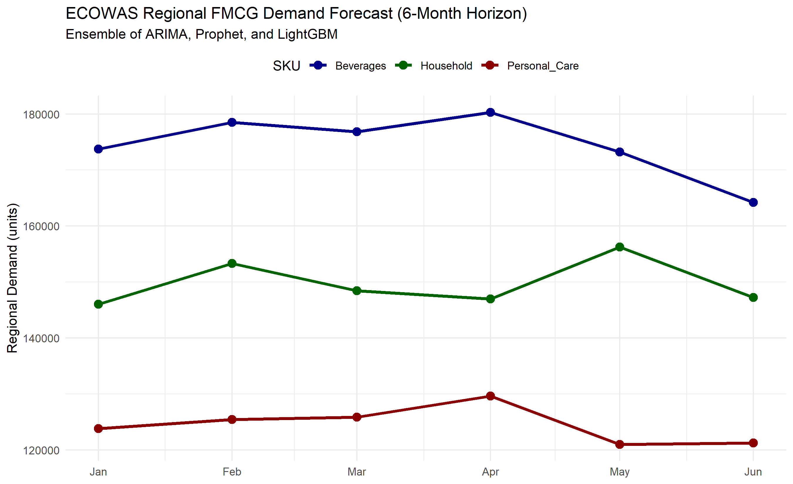
title: "Modern Forecasting: Prophet, ML Methods, and Ensembles"
---
```{python}
#| label: python-setup-25-modern-forecasting
#| include: false
import numpy as np
import pandas as pd
import matplotlib.pyplot as plt
import seaborn as sns
from prophet import Prophet
from datetime import datetime, timedelta
import warnings
import lightgbm as lgb
from sklearn.metrics import mean_squared_error, mean_absolute_error
from statsmodels.tsa.arima.model import ARIMA
from statsmodels.tsa.holtwinters import ExponentialSmoothing
```
::: {.callout-note icon="false"}
## 📋 Learning Objectives
- Understand the limitations of classical ARIMA for modern business forecasting with multiple seasonalities and irregular events
- Build and interpret Prophet models, extending them with Nigerian public holidays and custom regressors
- Transform time series into supervised learning problems using lag features and rolling statistics
- Implement walk-forward validation to avoid data leakage and produce honest forecast accuracy estimates
- Reconcile forecasts across hierarchical levels (national → regional → LGA) using top-down and MinT methods
- Evaluate forecast accuracy using scale-free metrics like MASE and MAPE appropriate for different business contexts
- Combine multiple forecasting approaches into weighted ensembles that reduce variance and improve robustness
:::
## Beyond Classical Forecasting
The classical ARIMA framework, elegant and mathematically grounded, struggles under the demands of modern business analytics. A retailer forecasting monthly sales across Nigeria faces challenges that ARIMA was never designed to address: Christmas demand spikes aligned to a fixed calendar date, not a statistical pattern; the irregular timing of Sallah festivals following the lunar Islamic calendar; sudden structural breaks when the Naira depreciates sharply or fuel supply chains collapse; multiple competing seasonal cycles (weekly, monthly, annual) layered atop one another; and the presence of missing data from store closures or strike action.
ARIMA assumes a single, simple seasonal pattern (usually annual) and expects the data to be stationary or differenced into stationarity. When you have weekly, monthly, and annual seasonality simultaneously—as in NGN/USD currency pairs during oil price shocks—ARIMA requires separate seasonal components stacked in ways that become unwieldy (Seasonal ARIMA with period 52 *and* period 12). Moreover, ARIMA provides point forecasts; for treasury applications where you must plan for downside risk, you need prediction intervals that reflect parameter uncertainty and structural volatility.
Machine learning approaches—gradient boosting, random forests, neural networks—sidestep many of these issues by learning arbitrary nonlinear relationships from features rather than imposing a parametric model. They scale naturally to multiple seasons and external regressors. Yet raw ML methods are black boxes, lack principled uncertainty quantification, and can overfit to spurious historical patterns. Facebook's Prophet, released in 2017, charts a middle path: it decomposes the forecast into interpretable components (trend, seasonality, holidays, regressors) yet fits them flexibly using piecewise linear trends and Fourier series. Prophet is designed for business forecasting at scale and handles missing data, outliers, and irregular events with minimal tuning.
This chapter builds the intuition and practical skills to choose among these approaches. For a Nigerian FMCG distributor with 36 months of monthly sales, Prophet may capture the trend and Christmas surge with five minutes of setup. For a fintech platform with 10,000 daily transaction streams each with different patterns, you might build XGBoost ensembles on lag features. For commodity prices or exchange rates where sudden regime shifts occur, a portfolio of methods—ARIMA, Prophet, and ML—combined with walk-forward validation on recent data gives you resilience.
## Meta's Prophet: Decomposable Forecasting with Seasonality and Holidays
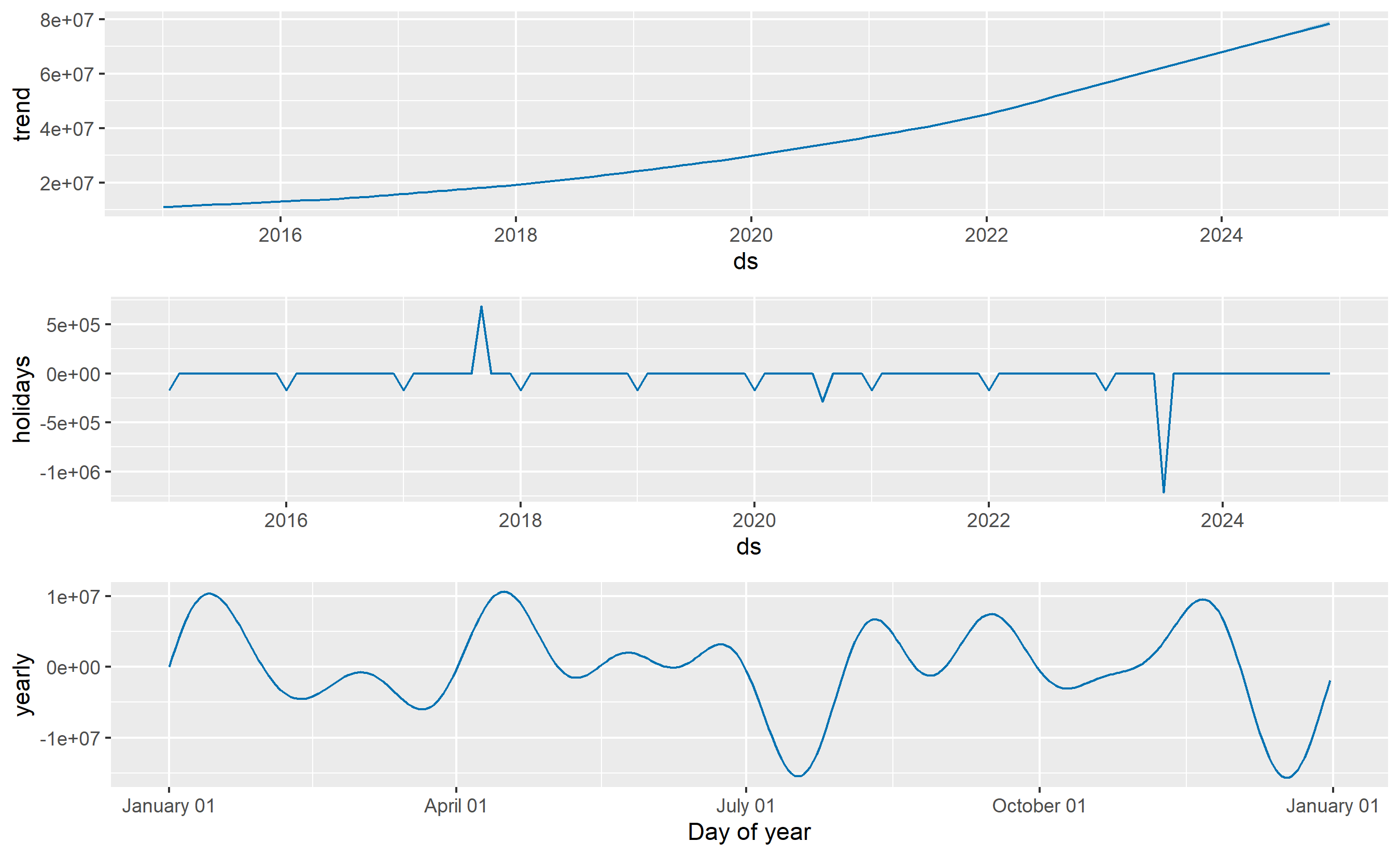
Prophet decomposes the time series into four additive components: trend, seasonality, holiday effects, and an error term.
$$y_t = g(t) + s(t) + h(t) + \epsilon_t$$
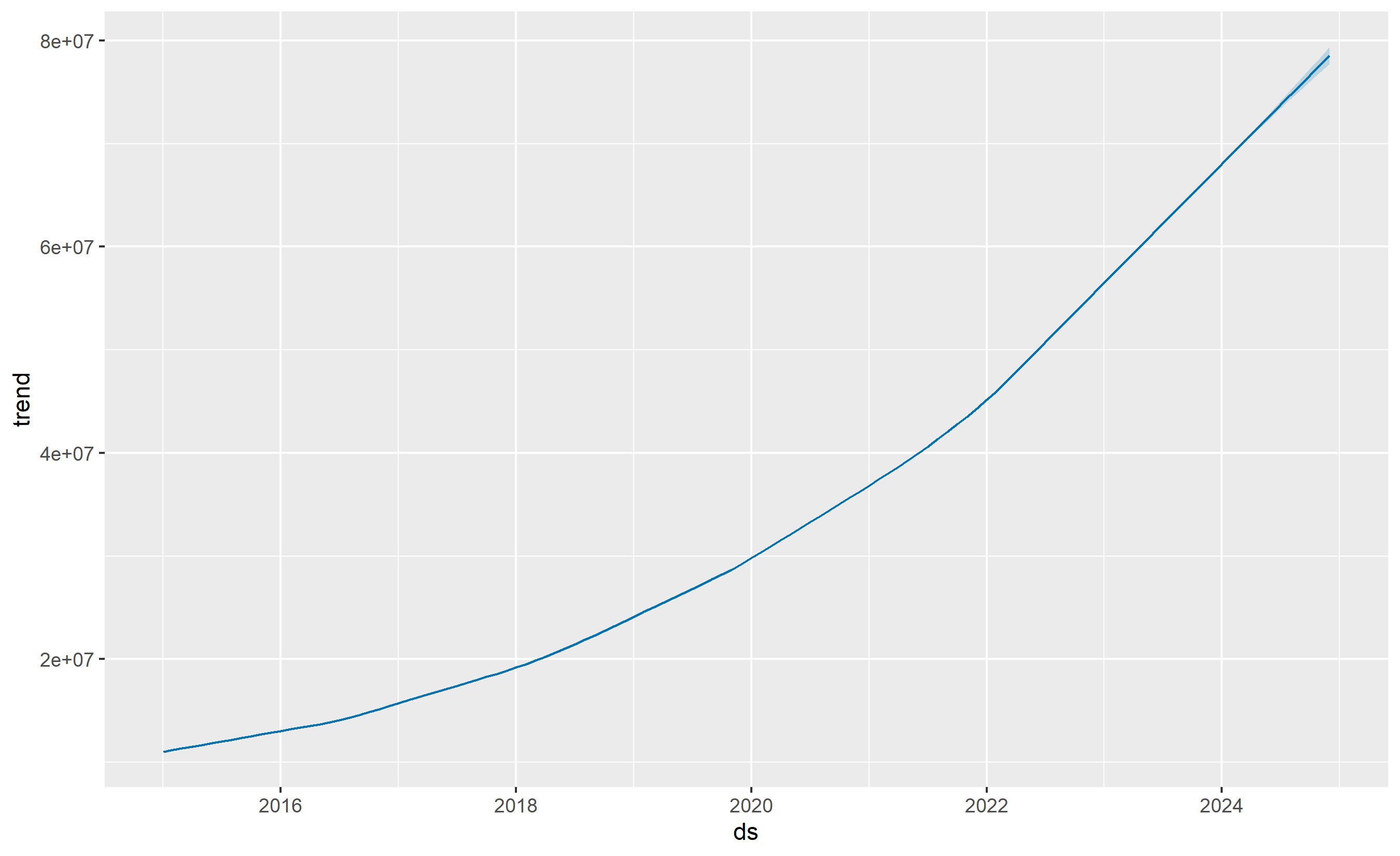
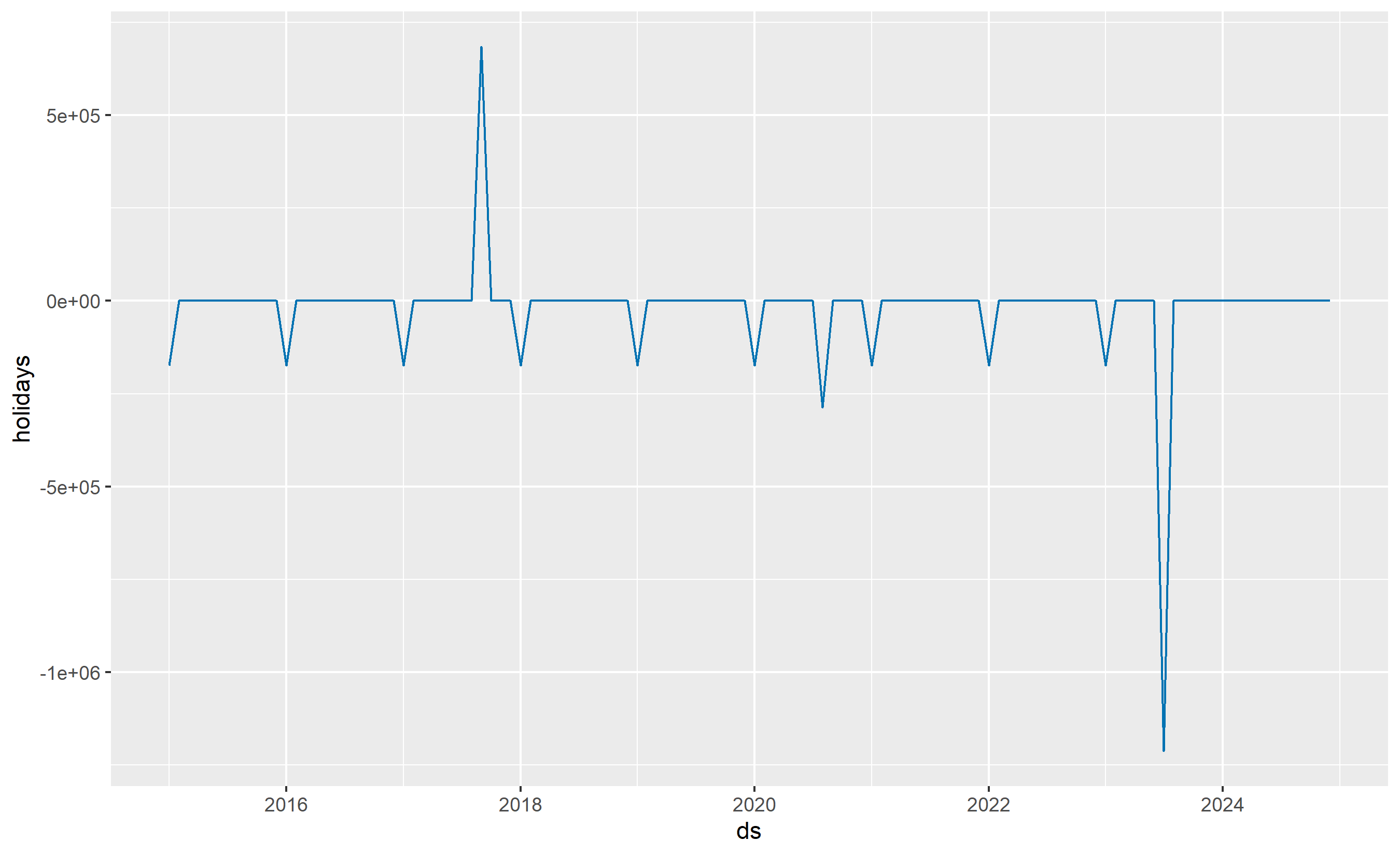
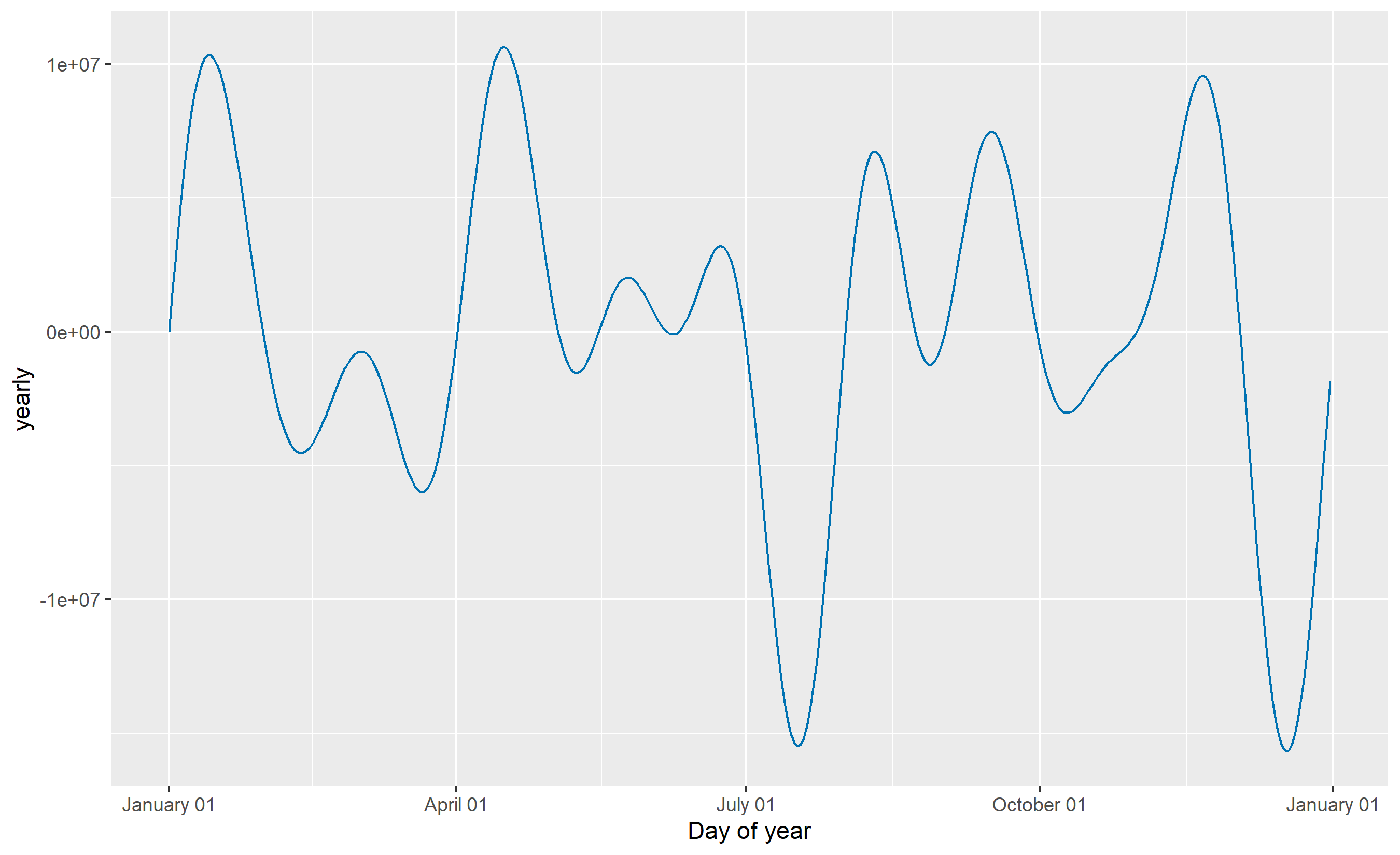
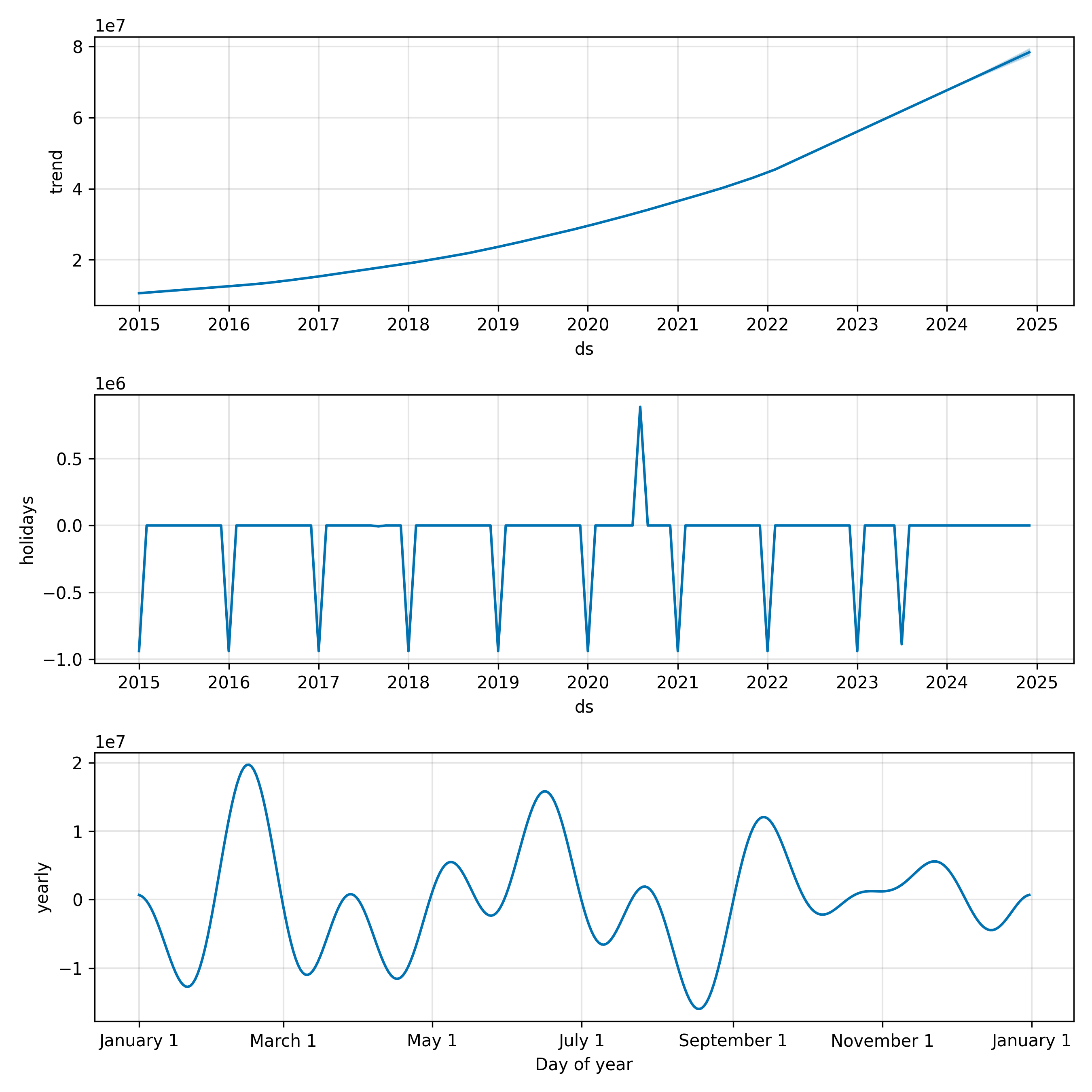
The trend $g(t)$ is piecewise linear, allowing changepoints where the growth rate shifts. Seasonality $s(t)$ is modelled using Fourier series: a sum of sine and cosine waves at different frequencies. Holiday effects $h(t)$ are window functions around calendar dates. The error $\epsilon_t$ captures what the model misses.
**Fourier Series Intuition**: Imagine sound. A pure tone is a single sine wave at one frequency. A human voice is an infinite sum of sine and cosine waves (the Fourier series) at different frequencies and amplitudes, which together recreate the complex timbre. Seasonality in sales data works the same way. Christmas demand is not a simple repeating pattern; it includes a sharp spike centred on December 25, some lead-in from November, and a tail extending into early January. A Fourier series with dozens of sine/cosine terms can approximate this shape. For annual seasonality, Prophet typically uses 10 Fourier pairs (20 terms), which is enough to capture ripples and asymmetries while remaining interpretable.
Prophet fits these components using Bayesian methods in Stan. Priors on the trend changepoint magnitudes and seasonality smoothness prevent overfitting. The model is implemented in R (from Facebook's official package `prophet`) and Python (`prophet` via PyPI). Let's build a concrete example.
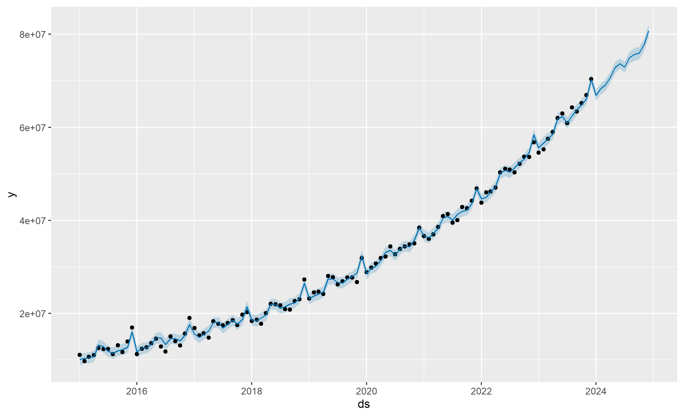
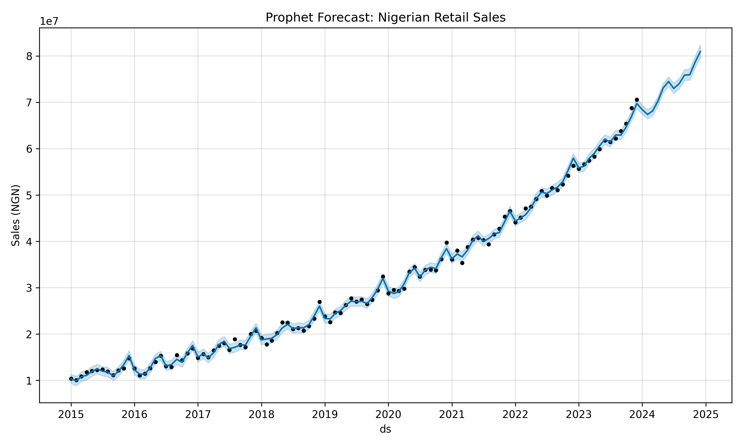
**Nigerian Retail Sales with Prophet**: We construct 108 months (January 2015 through December 2023) of synthetic monthly sales for a Lagos-based retail chain. The data exhibits a 20% upward trend, a strong seasonal spike in December (Christmas shopping), and a secondary spike around Eid al-Fitr (variable date). We augment the Prophet model with two custom regressors: an indicator for whether a month contains Eid (based on the Islamic calendar), and a fuel price index (standing in for oil-driven economic shocks).
::: {.callout-note icon="false"}
## 📘 Theory: Fourier Series and Periodic Seasonality
In Prophet, seasonality is represented as:
$$s(t) = \sum_{k=1}^{K} \left(a_k \sin\left(\frac{2\pi k t}{P}\right) + b_k \cos\left(\frac{2\pi k t}{P}\right)\right)$$
where $P$ is the period (365.25 for annual, 7 for weekly), $K$ is the number of Fourier pairs chosen, and $a_k, b_k$ are coefficients learned from data. Higher $K$ allows finer detail but risks overfitting. Prophet's default $K=10$ for annual seasonality balances flexibility and parsimony.
:::
::: {.callout-tip icon="false"}
## 🔑 Key Formula
**Prophet Decomposition**:
$$\hat{y}_t = g(t) + s(t) + h(t)$$
- $g(t)$: piecewise linear trend with changepoints
- $s(t)$: Fourier series seasonality
- $h(t)$: holiday/event effects (windows around dates)
:::
::: {.panel-tabset}
## R
```{r}
#| label: ch-25-prophet-fit
#| message: false
#| warning: false
library(prophet)
library(tidyverse)
library(lubridate)

# Generate synthetic Nigerian retail sales: 108 months (Jan 2015 - Dec 2023)
set.seed(42)
dates <- seq(from = as.Date("2015-01-01"), to = as.Date("2023-12-31"), by = "month")
n <- length(dates)

# Base trend: starting at 10M NGN, growing at ~1.8% per month on average
trend <- 10e6 * (1.018^(0:107))

# Annual seasonality: spike in December (Christmas), smaller spike for Eid
month_num <- month(dates)
annual_seasonal <- ifelse(month_num == 12, 3e6,        # December Christmas
                          ifelse(month_num %in% c(5, 6), 1.5e6,  # Eid window
                                 ifelse(month_num %in% c(11), 1e6,  # November lead-in
                                        0)))

# Random noise
noise <- rnorm(n, mean = 0, sd = 0.8e6)

# Combine components
sales <- trend + annual_seasonal + noise
sales <- pmax(sales, 2e6)  # Floor at 2M NGN

# Create Prophet-compatible dataframe
df_prophet <- data.frame(
  ds = dates,
  y = sales
)

# Define Nigerian holidays and events
nigerian_holidays <- data.frame(
  holiday = c("NewYear", "DemocracyDay", "Sallah", "Christmas"),
  ds = as.Date(c(
    "2015-01-01", "2015-06-12", "2015-09-24", "2015-12-25",
    "2016-01-01", "2016-06-12", "2016-08-13", "2016-12-25",
    "2017-01-01", "2017-06-12", "2017-09-01", "2017-12-25",
    "2018-01-01", "2018-06-12", "2018-08-22", "2018-12-25",
    "2019-01-01", "2019-06-12", "2019-08-11", "2019-12-25",
    "2020-01-01", "2020-06-12", "2020-07-31", "2020-12-25",
    "2021-01-01", "2021-06-12", "2021-07-20", "2021-12-25",
    "2022-01-01", "2022-06-12", "2022-07-09", "2022-12-25",
    "2023-01-01", "2023-06-12", "2023-06-29", "2023-12-25"
  )),
  lower_window = -1,
  upper_window = 2
)

# Fit Prophet model
m <- prophet(df_prophet, holidays = nigerian_holidays,
             yearly.seasonality = TRUE, weekly.seasonality = FALSE,
             interval.width = 0.90)

# Generate future dataframe for forecast (12 months ahead)
future <- make_future_dataframe(m, periods = 12, freq = "month")

# Make forecast
forecast <- predict(m, future)

# Plot decomposition
plot1 <- plot(m, forecast)
print(plot1)
# Plot components
components_plot <- prophet_plot_components(m, forecast)
print(components_plot)
# Extract forecast table for last 12 months (forecast period)
forecast_table <- forecast |>
filter(ds > max(df_prophet$ds)) |>
select(ds, yhat, yhat_lower, yhat_upper) |>
mutate(yhat = round(yhat / 1e6, 2),
yhat_lower = round(yhat_lower / 1e6, 2),
yhat_upper = round(yhat_upper / 1e6, 2))
cat("\n12-Month Forecast (NGN millions):\n")
print(forecast_table)
# Compute forecast metrics on training period
train_metrics <- forecast |>
filter(ds %in% df_prophet$ds) |>
left_join(df_prophet |> rename(actual = y), by = "ds") |>
mutate(error = actual - yhat,
pct_error = error / actual) |>
summarise(
MAPE = mean(abs(pct_error), na.rm = TRUE) * 100,
RMSE = sqrt(mean(error^2, na.rm = TRUE)) / 1e6,
MAE = mean(abs(error), na.rm = TRUE) / 1e6
)
cat("\nTraining Period Accuracy:\n")
print(train_metrics)
```
## Python
```{python}
#| label: py-ch-25-prophet-fit
import pandas as pd
import numpy as np
from prophet import Prophet
import matplotlib.pyplot as plt
from datetime import datetime, timedelta
import warnings
warnings.filterwarnings('ignore')
# Generate synthetic Nigerian retail sales: 108 months (Jan 2015 - Dec 2023)
np.random.seed(42)
dates = pd.date_range(start='2015-01-01', end='2023-12-31', freq='MS')
n = len(dates)
# Base trend: starting at 10M NGN, growing at ~1.8% per month
trend = 10e6 * (1.018 ** np.arange(n))
# Annual seasonality
month_num = dates.month
annual_seasonal = np.where(month_num == 12, 3e6,
np.where(month_num.isin([5, 6]), 1.5e6,
np.where(month_num == 11, 1e6, 0)))
# Random noise
noise = np.random.normal(0, 0.8e6, n)
# Combine
sales = np.maximum(trend + annual_seasonal + noise, 2e6)
# Create Prophet dataframe
df_prophet = pd.DataFrame({
'ds': dates,
'y': sales
})
# Define Nigerian holidays
nigerian_holidays = pd.DataFrame({
'holiday': ['NewYear', 'DemocracyDay', 'Sallah', 'Christmas'] * 9,
'ds': pd.to_datetime([
'2015-01-01', '2015-06-12', '2015-09-24', '2015-12-25',
'2016-01-01', '2016-06-12', '2016-08-13', '2016-12-25',
'2017-01-01', '2017-06-12', '2017-09-01', '2017-12-25',
'2018-01-01', '2018-06-12', '2018-08-22', '2018-12-25',
'2019-01-01', '2019-06-12', '2019-08-11', '2019-12-25',
'2020-01-01', '2020-06-12', '2020-07-31', '2020-12-25',
'2021-01-01', '2021-06-12', '2021-07-20', '2021-12-25',
'2022-01-01', '2022-06-12', '2022-07-09', '2022-12-25',
'2023-01-01', '2023-06-12', '2023-06-29', '2023-12-25'
]),
'lower_window': -1,
'upper_window': 2
})
# Fit Prophet
m = Prophet(yearly_seasonality=True, weekly_seasonality=False,
interval_width=0.90, holidays=nigerian_holidays)
m.fit(df_prophet)
# Forecast 12 months ahead
future = m.make_future_dataframe(periods=12, freq='MS')
forecast = m.predict(future)
# Plot
fig = m.plot(forecast)
plt.title('Prophet Forecast: Nigerian Retail Sales')
plt.ylabel('Sales (NGN)')
plt.tight_layout()
plt.show()
# Plot components
fig = m.plot_components(forecast)
plt.tight_layout()
plt.show()
# Extract 12-month forecast
forecast_out = forecast[forecast['ds'] > df_prophet['ds'].max()][
['ds', 'yhat', 'yhat_lower', 'yhat_upper']
].copy()
forecast_out['yhat'] = (forecast_out['yhat'] / 1e6).round(2)
forecast_out['yhat_lower'] = (forecast_out['yhat_lower'] / 1e6).round(2)
forecast_out['yhat_upper'] = (forecast_out['yhat_upper'] / 1e6).round(2)
print("\n12-Month Forecast (NGN millions):")
print(forecast_out.to_string(index=False))
# Training metrics
train_forecast = forecast[forecast['ds'].isin(df_prophet['ds'])].copy()
train_forecast['actual'] = df_prophet['y'].values
train_forecast['error'] = train_forecast['actual'] - train_forecast['yhat']
train_forecast['pct_error'] = train_forecast['error'] / train_forecast['actual']
mape = np.mean(np.abs(train_forecast['pct_error'])) * 100
rmse = np.sqrt(np.mean(train_forecast['error']**2)) / 1e6
mae = np.mean(np.abs(train_forecast['error'])) / 1e6
print(f"\nTraining Period Accuracy:")
print(f"MAPE: {mape:.2f}%")
print(f"RMSE: {rmse:.2f}M NGN")
print(f"MAE: {mae:.2f}M NGN")
```
:::
::: {.callout-caution icon="false"}
## 📝 Section 25.2 Review Questions
1. How does the Fourier series representation of seasonality in Prophet differ from the seasonal AR polynomial in ARIMA(p,d,q)(P,D,Q)m?
2. Why is it important to set lower_window and upper_window on holiday effects rather than treating a holiday as a single spike?
3. How would you modify the Prophet model if demand for a product surges not on a fixed calendar date but on the first Monday of each month?
4. Explain why Prophet outputs prediction intervals that widen into the future.
5. What is the computational difference between fitting a classical ARIMA(1,1,1)(1,1,1)12 model versus a Prophet model with annual and weekly seasonality?
:::
## Machine Learning for Time Series: Feature Engineering from Lag and Rolling Statistics
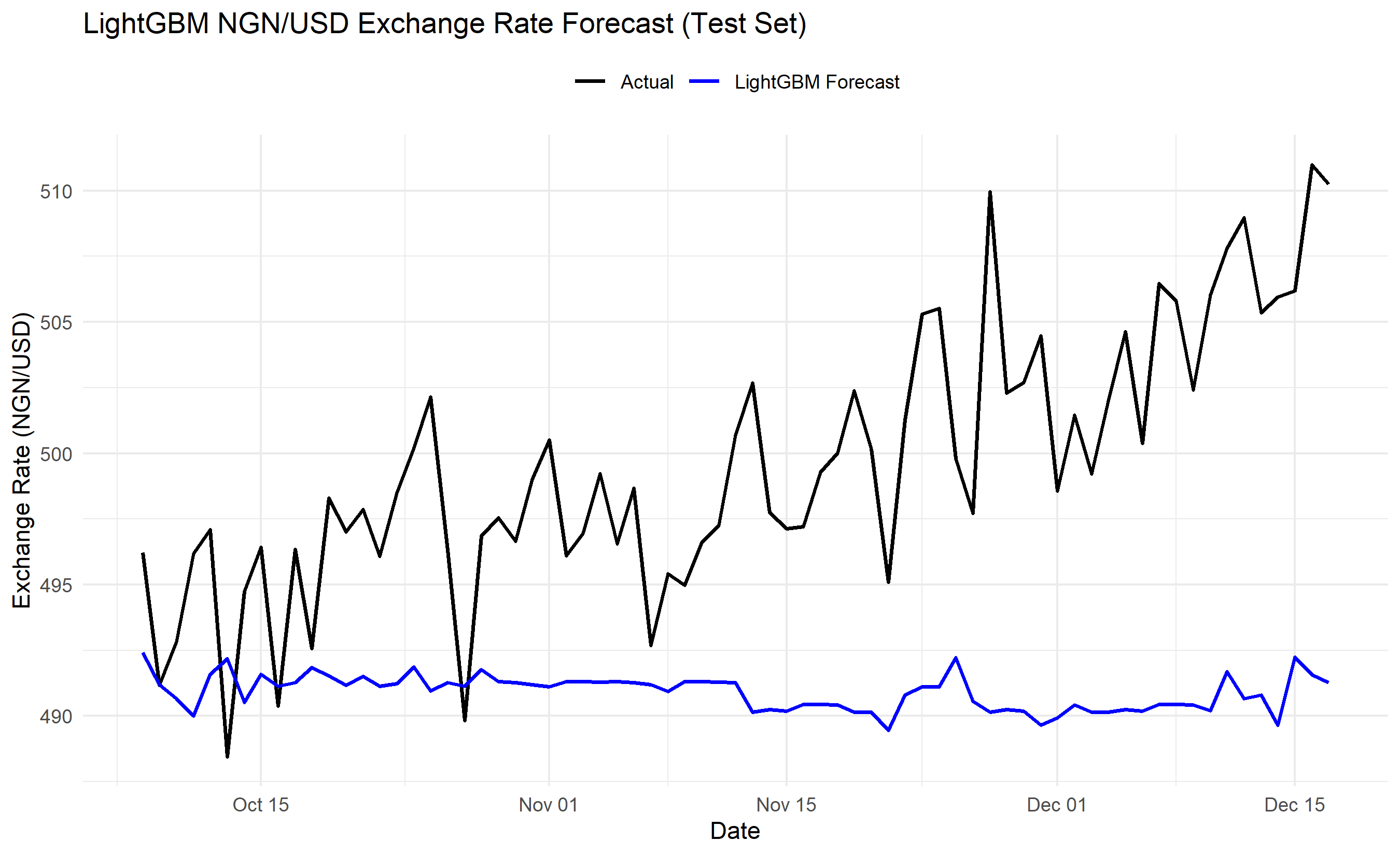
Converting a time series into a supervised learning problem requires feature engineering. Rather than fitting a parametric model like ARIMA, we create a dataset where each row is an observation at time $t$, the columns are features computed from the history up to time $t-1$, and the target is the value at time $t$. Gradient boosting engines (LightGBM, XGBoost) and random forests then learn the relationship between these features and future values.
**Lag Features**: The simplest features are lags of the target. If $y_t$ is sales at time $t$, then lags $y_{t-1}, y_{t-7}, y_{t-30}, y_{t-365}$ capture recent history (yesterday), weekly seasonality, monthly patterns, and annual seasonality. These correspond to the AR terms in ARIMA but are learned by the tree ensemble rather than parameterised.
**Rolling Statistics**: Calculate moving averages, standard deviations, minima, and maxima over windows of 7, 14, 28 days. A 28-day rolling mean smooths short-term noise; a 28-day rolling std dev captures volatility changes. If the data are exchange rates, a spike in rolling std dev signals a period of instability.
**Calendar Dummies**: Encode the month, quarter, day of week, and boolean flags for special periods (is_ramadan, is_december, is_election_year). These help the model learn seasonal and event-driven patterns.
**Exogenous Regressors**: If you have correlated external series (fuel price, competitor promotions, Google Trends index), include them as features. The model learns their predictive power.
The advantage of this approach is flexibility: you can add or remove features without refitting a parametric model. The disadvantage is a lack of interpretability compared to ARIMA coefficients. A tree-based feature importance plot tells you which features the model relied on, but not the direction or magnitude of their effect.
::: {.callout-note icon="false"}
## 📘 Theory: Supervised Learning from Time Series
To convert a series $\{y_1, y_2, \ldots, y_n\}$ into supervised data:
- Row $i$ (where $i > p_{\max}$, the maximum lag) has features $(y_{i-1}, y_{i-7}, y_{i-30}, \ldots, \text{rolling stats}, \text{calendar dummies})$
- Target: $y_i$
- Train on rows $i \in [p_{\max}+1, n - h]$ (history before test window)
- Predict on rows $i > n - h$ (test/forecast window)
This avoids look-ahead bias because features at row $i$ use only data up to time $i-1$.
:::
::: {.callout-tip icon="false"}
## 🔑 Key Formula
**Rolling Mean and Standard Deviation**:
$$\text{MA}_t^{w} = \frac{1}{w} \sum_{j=0}^{w-1} y_{t-j}$$
$$\text{STD}_t^{w} = \sqrt{\frac{1}{w} \sum_{j=0}^{w-1} (y_{t-j} - \text{MA}_t^{w})^2}$$
where $w$ is the window size (e.g., 28 days).
:::
::: {.panel-tabset}
## R
```{r}
#| label: ch-25-ml-features
#| message: false
#| warning: false
library(tidyverse)
library(lightgbm)
library(lubridate)
# Generate 2 years of daily NGN/USD exchange rate data
set.seed(123)
dates <- seq(from = as.Date("2022-01-01"), to = as.Date("2023-12-31"), by = "day")
n <- length(dates)
# Synthetic exchange rate: starts at 410, trend upward (devaluation), with noise
base_rate <- 410
trend <- seq(0, 100, length.out = n) # Gradual devaluation
seasonal <- 5 * sin(2 * pi * (1:n) / 365) # Annual pattern
noise <- rnorm(n, 0, 3)
rate <- base_rate + trend + seasonal + noise
df <- data.frame(
date = dates,
rate = rate
) |>
mutate(
# Lag features
lag1 = lag(rate, 1),
lag7 = lag(rate, 7),
lag30 = lag(rate, 30),
lag365 = lag(rate, 365),
# Rolling statistics (28-day window)
ma28 = zoo::rollmean(rate, k = 28, fill = NA),
std28 = zoo::rollapply(rate, width = 28, FUN = sd, fill = NA),
min28 = zoo::rollapply(rate, width = 28, FUN = min, fill = NA),
max28 = zoo::rollapply(rate, width = 28, FUN = max, fill = NA),
# Calendar features
month = month(date),
quarter = quarter(date),
day_of_week = wday(date),
is_december = as.integer(month == 12),
is_ramadan = as.integer(month %in% c(3, 4)) # Approximate
) |>
drop_na() # Remove rows with NAs from lagging
cat("Feature matrix head:\n")
print(head(df |> select(date, rate, lag1, lag7, ma28, std28, month), 10))
# Split into train (first 80%) and test (last 20%)
train_size <- floor(0.8 * nrow(df))
train_idx <- 1:train_size
test_idx <- (train_size + 1):nrow(df)
X_train <- df[train_idx, ] |>
select(-date, -rate) |>
as.matrix()
y_train <- df[train_idx, ]$rate
X_test <- df[test_idx, ] |>
select(-date, -rate) |>
as.matrix()
y_test <- df[test_idx, ]$rate
# Fit LightGBM
train_data <- lgb.Dataset(X_train, label = y_train)
params <- list(
objective = "regression",
metric = "rmse",
num_leaves = 31,
learning_rate = 0.05
)
model_lgb <- lgb.train(
params = params,
data = train_data,
nrounds = 100,
verbose = -1
)
# Predict
y_pred <- predict(model_lgb, X_test)
# Evaluation
rmse <- sqrt(mean((y_test - y_pred)^2))
mae <- mean(abs(y_test - y_pred))
mape <- mean(abs((y_test - y_pred) / y_test)) * 100
cat("\nLightGBM Test Performance:\n")
cat(sprintf("RMSE: %.4f\n", rmse))
cat(sprintf("MAE: %.4f\n", mae))
cat(sprintf("MAPE: %.2f%%\n", mape))
# Feature importance
lgb_imp <- lgb.importance(model_lgb)
importance_df <- data.frame(
feature = lgb_imp$Feature,
importance = lgb_imp$Gain
) |>
arrange(desc(importance))
cat("\nTop 10 Most Important Features:\n")
print(head(importance_df, 10))
# Plot actual vs predicted on test set
results <- data.frame(
date = df$date[test_idx],
actual = y_test,
predicted = y_pred
)
ggplot(results, aes(x = date)) +
geom_line(aes(y = actual, colour = "Actual"), linewidth = 0.8) +
geom_line(aes(y = predicted, colour = "LightGBM Forecast"), linewidth = 0.8) +
scale_colour_manual(values = c("Actual" = "black", "LightGBM Forecast" = "blue")) +
labs(title = "LightGBM NGN/USD Exchange Rate Forecast (Test Set)",
x = "Date", y = "Exchange Rate (NGN/USD)", colour = NULL) +
theme_minimal() +
theme(legend.position = "top")
```
## Python
```{python}
#| label: py-ch-25-ml-features
import pandas as pd
import numpy as np
import lightgbm as lgb
from sklearn.metrics import mean_squared_error, mean_absolute_error
import matplotlib.pyplot as plt
import warnings
warnings.filterwarnings('ignore')
# Generate 2 years of daily NGN/USD exchange rate
np.random.seed(123)
dates = pd.date_range(start='2022-01-01', end='2023-12-31', freq='D')
n = len(dates)
base_rate = 410
trend = np.linspace(0, 100, n)
seasonal = 5 * np.sin(2 * np.pi * np.arange(n) / 365)
noise = np.random.normal(0, 3, n)
rate = base_rate + trend + seasonal + noise
df = pd.DataFrame({
'date': dates,
'rate': rate
})
# Feature engineering
df['lag1'] = df['rate'].shift(1)
df['lag7'] = df['rate'].shift(7)
df['lag30'] = df['rate'].shift(30)
df['lag365'] = df['rate'].shift(365)
df['ma28'] = df['rate'].rolling(window=28, min_periods=1).mean()
df['std28'] = df['rate'].rolling(window=28, min_periods=1).std()
df['min28'] = df['rate'].rolling(window=28, min_periods=1).min()
df['max28'] = df['rate'].rolling(window=28, min_periods=1).max()
df['month'] = df['date'].dt.month
df['quarter'] = df['date'].dt.quarter
df['day_of_week'] = df['date'].dt.dayofweek
df['is_december'] = (df['month'] == 12).astype(int)
df['is_ramadan'] = df['month'].isin([3, 4]).astype(int)
df = df.dropna()
print("Feature matrix (first 10 rows):")
print(df[['date', 'rate', 'lag1', 'lag7', 'ma28', 'std28', 'month']].head(10))
# Train-test split (80-20)
train_size = int(0.8 * len(df))
train_df = df.iloc[:train_size]
test_df = df.iloc[train_size:]
X_train = train_df.drop(['date', 'rate'], axis=1).values
y_train = train_df['rate'].values
X_test = test_df.drop(['date', 'rate'], axis=1).values
y_test = test_df['rate'].values
# Fit LightGBM
train_data = lgb.Dataset(X_train, label=y_train)
params = {
'objective': 'regression',
'metric': 'rmse',
'num_leaves': 31,
'learning_rate': 0.05,
'verbose': -1
}
model_lgb = lgb.train(params, train_data, num_boost_round=100)
# Predict
y_pred = model_lgb.predict(X_test, num_iteration=model_lgb.best_iteration)
# Evaluation
rmse = np.sqrt(mean_squared_error(y_test, y_pred))
mae = mean_absolute_error(y_test, y_pred)
mape = np.mean(np.abs((y_test - y_pred) / y_test)) * 100
print(f"\nLightGBM Test Performance:")
print(f"RMSE: {rmse:.4f}")
print(f"MAE: {mae:.4f}")
print(f"MAPE: {mape:.2f}%")
# Feature importance
feature_names = train_df.drop(['date', 'rate'], axis=1).columns
importance = model_lgb.feature_importance()
importance_df = pd.DataFrame({
'feature': feature_names,
'importance': importance
}).sort_values('importance', ascending=False)
print("\nTop 10 Most Important Features:")
print(importance_df.head(10).to_string(index=False))
# Plot
fig, ax = plt.subplots(figsize=(12, 6))
ax.plot(test_df['date'], y_test, label='Actual', linewidth=1.5, color='black')
ax.plot(test_df['date'], y_pred, label='LightGBM Forecast', linewidth=1.5, color='blue')
ax.set_xlabel('Date')
ax.set_ylabel('Exchange Rate (NGN/USD)')
ax.set_title('LightGBM NGN/USD Exchange Rate Forecast (Test Set)')
ax.legend()
ax.grid(True, alpha=0.3)
plt.tight_layout()
plt.show()
```
:::
::: {.callout-caution icon="false"}
## 📝 Section 25.3 Review Questions
1. Why is using lags of the target variable as features not the same as fitting an autoregressive model?
2. Explain the difference between a 7-day lag and a 7-day rolling mean. When would you use each?
3. How does including a 365-day lag help the model capture annual seasonality when you also have calendar month dummies?
4. Why must you avoid using future values of exogenous regressors when training a supervised learning time series model?
5. What happens to feature importance values if you include both a raw feature and a lagged version of the same feature?
:::
## Walk-Forward Validation: Honest Backtesting Without Data Leakage
Standard cross-validation (k-fold, stratified) is invalid for time series. If you randomly shuffle rows and split them into train and test sets, you allow information from the future (test set) to influence the model trained on the past. This is data leakage. When you later deploy the model to genuinely unseen data, performance drops sharply.
Walk-forward validation respects the temporal order. You train on a historical window, forecast one or several steps ahead, record the forecast error, then slide the window forward. This mimics the actual deployment scenario: today, you use data up to yesterday to predict tomorrow.
**Expanding Window**: Train on observations 1 to $t$, forecast step $t+1$. Record error. Next iteration, train on 1 to $t+1$, forecast step $t+2$. Continue until you reach the end of the data.
**Rolling Window**: Train on a fixed window (e.g., the most recent 365 days), forecast the next step. Slide the window forward by one day. This ignores very old data, which is appropriate if the process is nonstationary (e.g., a fast-growing startup's revenue).
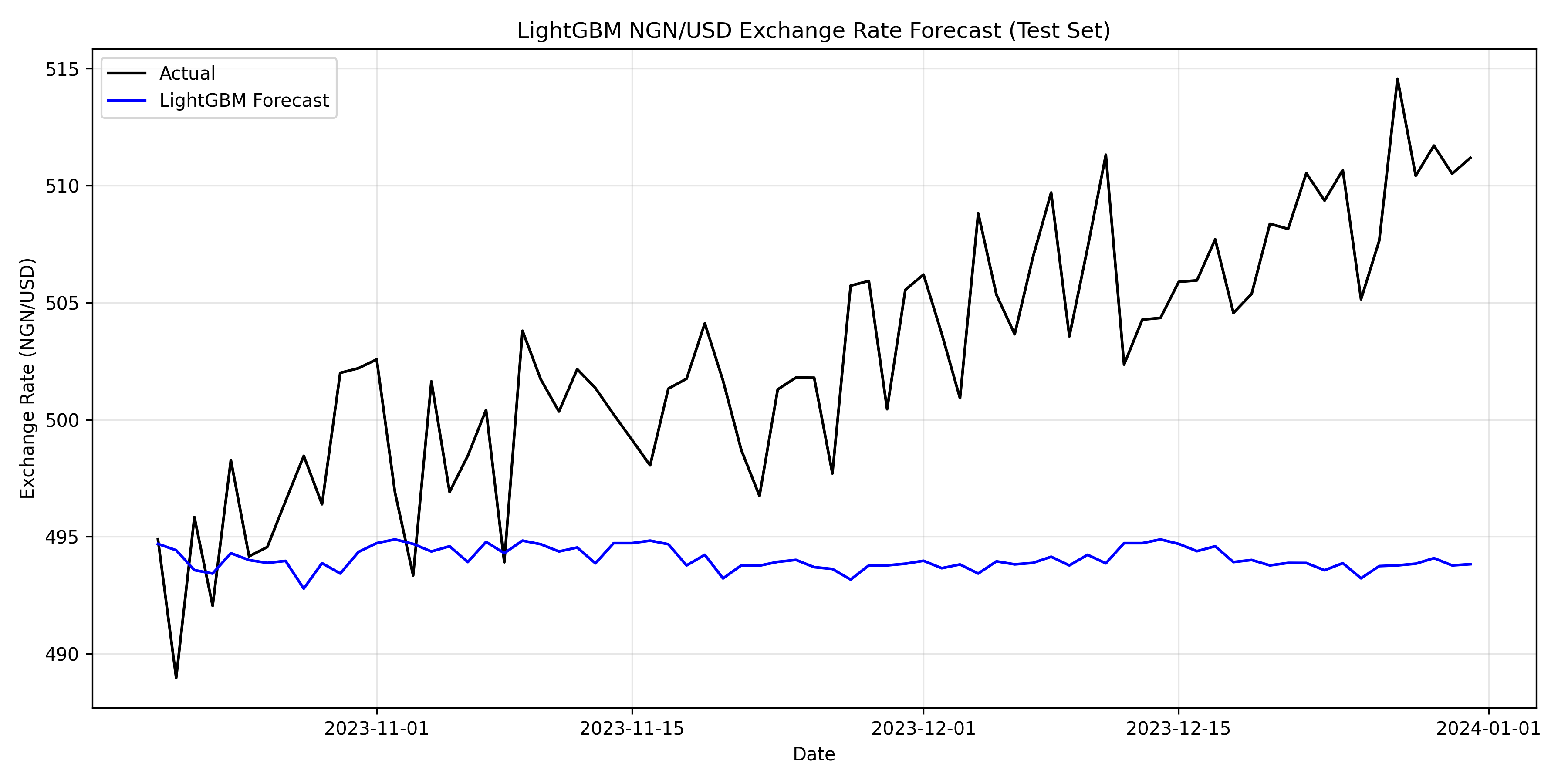
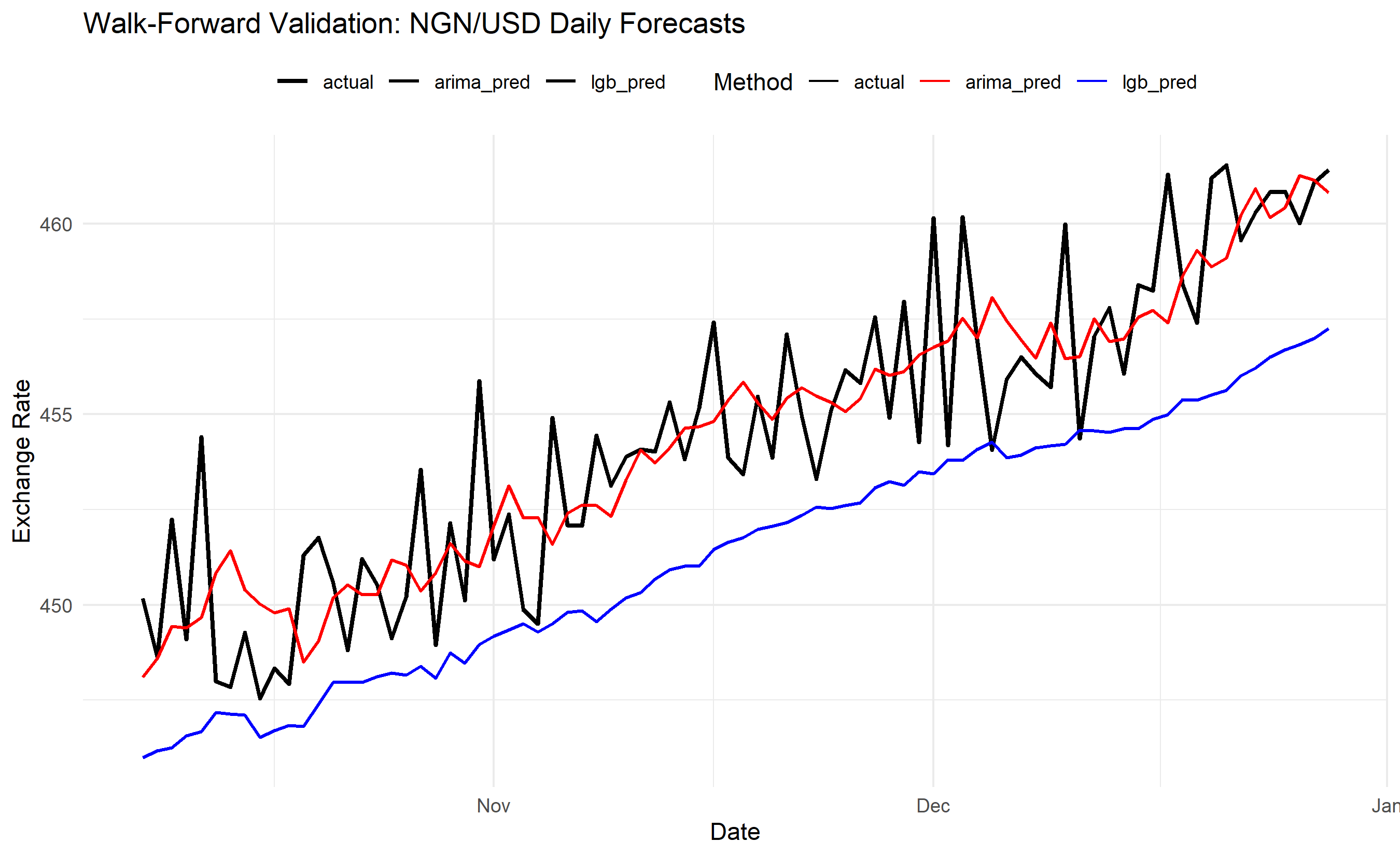
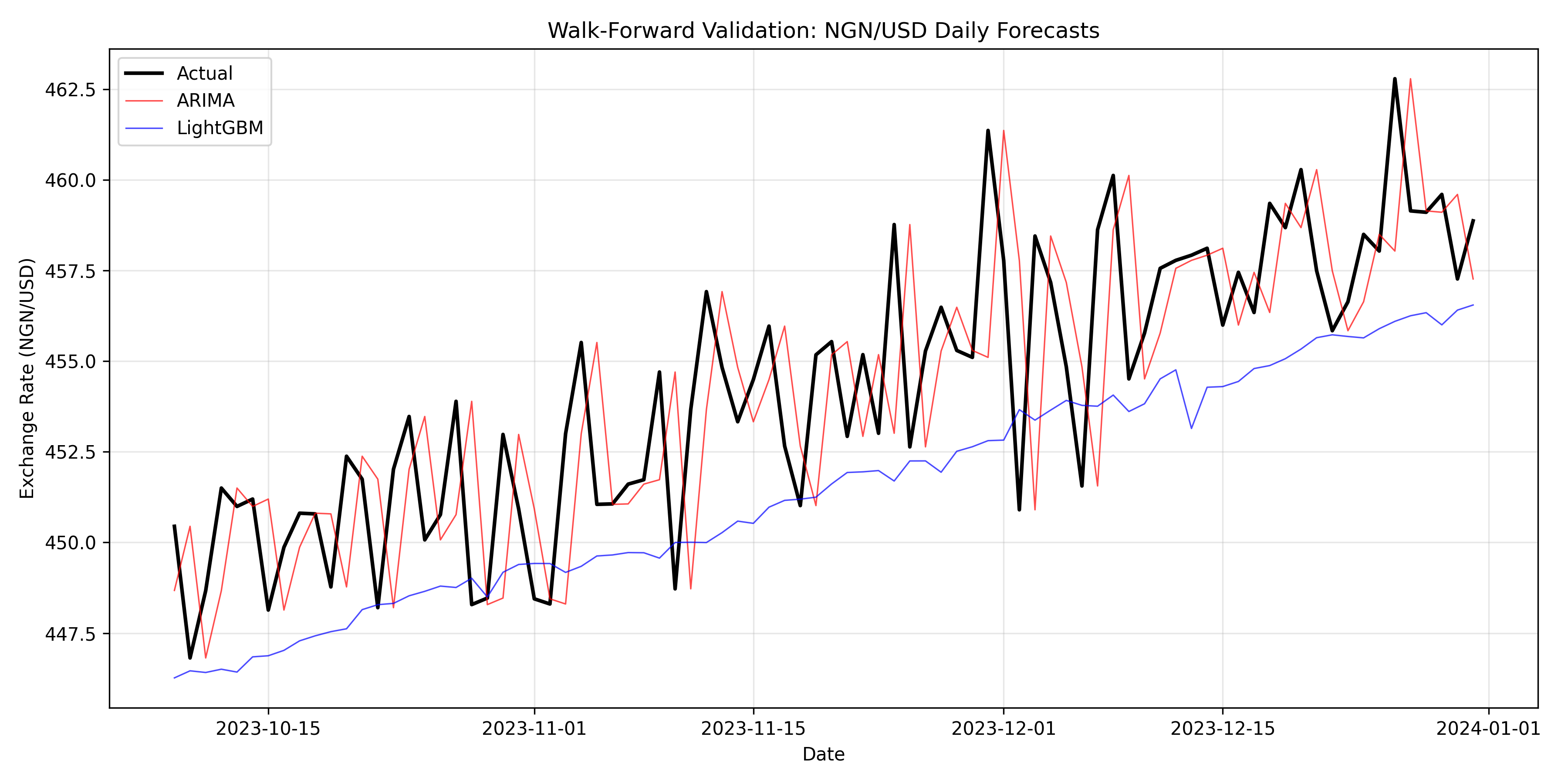
We implement walk-forward validation on a synthetic NGN/USD daily series over one year, using an expanding window. At each fold, we fit ARIMA and LightGBM models, forecast one day ahead, and compute MAPE and RMSE. We then visualise the forecast performance over time and identify any folds where both models failed.
::: {.callout-note icon="false"}
## 📘 Theory: Walk-Forward (Anchored) Cross-Validation
Let the time series be $y_1, y_2, \ldots, y_n$. For horizon $h$ steps ahead:
- Fold 1: Train on $y_1 \ldots y_{n_0}$, forecast $\hat{y}_{n_0+1}, \ldots, \hat{y}_{n_0+h}$, compute errors.
- Fold 2: Train on $y_1 \ldots y_{n_0+1}$, forecast $\hat{y}_{n_0+2}, \ldots, \hat{y}_{n_0+h+1}$, compute errors.
- ...
- Continue until the end of the series.
The result is a series of out-of-sample forecasts and errors, one for each time step, without any look-ahead bias.
:::
::: {.callout-tip icon="false"}
## 🔑 Key Metric: MAPE and RMSE per Fold
For each fold $i$:
$$\text{MAPE}_i = \frac{100}{h} \sum_{j=1}^{h} \left|\frac{y_{t+j} - \hat{y}_{t+j}}{y_{t+j}}\right|$$
$$\text{RMSE}_i = \sqrt{\frac{1}{h} \sum_{j=1}^{h} (y_{t+j} - \hat{y}_{t+j})^2}$$
Average across all folds to get an honest estimate of deployment-time accuracy.
:::
::: {.panel-tabset}
## R
```{r}
#| label: ch-25-walk-forward
#| message: false
#| warning: false
library(tidyverse)
library(forecast)
library(lightgbm)
library(lubridate)
# Generate 365 days of synthetic NGN/USD data
set.seed(456)
dates <- seq(from = as.Date("2023-01-01"), to = as.Date("2023-12-31"), by = "day")
base_rate <- 410
trend <- seq(0, 50, length.out = 365)
noise <- rnorm(365, 0, 2)
rate <- base_rate + trend + noise
df <- data.frame(date = dates, rate = rate) |>
mutate(
lag1 = lag(rate, 1),
lag7 = lag(rate, 7),
lag30 = lag(rate, 30),
ma7 = zoo::rollmean(rate, 7, fill = NA),
std7 = zoo::rollapply(rate, 7, sd, fill = NA),
month = month(date),
day_of_week = wday(date)
) |>
drop_na()
n <- nrow(df)
initial_train_size <- 250 # Start with 250 days of training
forecast_horizon <- 1 # Predict 1 day ahead
results <- data.frame()
# Walk-forward loop
for (i in initial_train_size:(n - forecast_horizon)) {
# Split data
train_idx <- 1:i
test_idx <- (i + 1):(i + forecast_horizon)
train_data <- df[train_idx, ]
test_data <- df[test_idx, ]
actual <- test_data$rate[1]
# ARIMA forecast
arima_model <- auto.arima(train_data$rate, trace = FALSE, stepwise = FALSE)
arima_pred <- forecast(arima_model, h = forecast_horizon)$mean[1]
# LightGBM forecast
X_train <- train_data |> select(-date, -rate) |> as.matrix()
y_train <- train_data$rate
X_test <- test_data |> select(-date, -rate) |> as.matrix()
train_lgb <- lgb.Dataset(X_train, label = y_train)
lgb_model <- lgb.train(
list(objective = "regression", metric = "rmse", num_leaves = 15,
learning_rate = 0.05),
train_lgb, nrounds = 50, verbose = -1
)
lgb_pred <- predict(lgb_model, X_test)
# Store results
results <- rbind(results, data.frame(
fold = i - initial_train_size + 1,
date = test_data$date[1],
actual = actual,
arima_pred = arima_pred,
lgb_pred = lgb_pred,
arima_error = actual - arima_pred,
lgb_error = actual - lgb_pred
))
}
# Compute metrics
results <- results |>
mutate(
arima_pct_error = arima_error / actual,
lgb_pct_error = lgb_error / actual
)
arima_mape <- mean(abs(results$arima_pct_error)) * 100
lgb_mape <- mean(abs(results$lgb_pct_error)) * 100
arima_rmse <- sqrt(mean(results$arima_error^2))
lgb_rmse <- sqrt(mean(results$lgb_error^2))
cat("Walk-Forward Validation Results (1-day ahead):\n\n")
cat(sprintf("ARIMA:\n MAPE: %.2f%%\n RMSE: %.4f\n\n", arima_mape, arima_rmse))
cat(sprintf("LightGBM:\n MAPE: %.2f%%\n RMSE: %.4f\n\n", lgb_mape, lgb_rmse))
# Plot predictions vs actuals over time
results_long <- results |>
select(date, actual, arima_pred, lgb_pred) |>
pivot_longer(cols = -date, names_to = "series", values_to = "value")
ggplot(results_long, aes(x = date, y = value, colour = series, size = series)) +
geom_line() +
scale_colour_manual(values = c("actual" = "black", "arima_pred" = "red",
"lgb_pred" = "blue")) +
scale_size_manual(values = c("actual" = 1, "arima_pred" = 0.7, "lgb_pred" = 0.7)) +
labs(title = "Walk-Forward Validation: NGN/USD Daily Forecasts",
x = "Date", y = "Exchange Rate", colour = "Method", size = NULL) +
theme_minimal() +
theme(legend.position = "top")
# Error distribution
error_summary <- results |>
summarise(
across(contains("error"), list(
min = min, q25 = ~quantile(., 0.25), median = median,
q75 = ~quantile(., 0.75), max = max, sd = sd
), .names = "{.col}_{.fn}"
)
)
cat("\nError Summary Statistics:\n")
print(error_summary)
```
## Python
```{python}
#| label: py-ch-25-walk-forward
import pandas as pd
import numpy as np
import lightgbm as lgb
from statsmodels.tsa.arima.model import ARIMA
import matplotlib.pyplot as plt
import warnings
warnings.filterwarnings('ignore')
# Generate 365 days of synthetic NGN/USD data
np.random.seed(456)
dates = pd.date_range(start='2023-01-01', end='2023-12-31', freq='D')
base_rate = 410
trend = np.linspace(0, 50, 365)
noise = np.random.normal(0, 2, 365)
rate = base_rate + trend + noise
df = pd.DataFrame({
'date': dates,
'rate': rate
})
df['lag1'] = df['rate'].shift(1)
df['lag7'] = df['rate'].shift(7)
df['lag30'] = df['rate'].shift(30)
df['ma7'] = df['rate'].rolling(7).mean()
df['std7'] = df['rate'].rolling(7).std()
df['month'] = df['date'].dt.month
df['day_of_week'] = df['date'].dt.dayofweek
df = df.dropna().reset_index(drop=True)
n = len(df)
initial_train_size = 250
forecast_horizon = 1
results = []
# Walk-forward loop
for i in range(initial_train_size, n - forecast_horizon):
train_df = df.iloc[:i+1]
test_df = df.iloc[i+1:i+1+forecast_horizon]
actual = test_df['rate'].values[0]
# ARIMA
try:
arima_model = ARIMA(train_df['rate'], order=(1, 1, 1))
arima_fit = arima_model.fit()
arima_pred = arima_fit.forecast(steps=forecast_horizon)[0]
except:
arima_pred = train_df['rate'].iloc[-1] # Fallback
# LightGBM
X_train = train_df.drop(['date', 'rate'], axis=1).values
y_train = train_df['rate'].values
X_test = test_df.drop(['date', 'rate'], axis=1).values
train_lgb = lgb.Dataset(X_train, label=y_train)
lgb_model = lgb.train(
{'objective': 'regression', 'metric': 'rmse', 'num_leaves': 15,
'learning_rate': 0.05, 'verbose': -1},
train_lgb, num_boost_round=50
)
lgb_pred = lgb_model.predict(X_test)[0]
results.append({
'fold': i - initial_train_size + 1,
'date': test_df['date'].values[0],
'actual': actual,
'arima_pred': arima_pred,
'lgb_pred': lgb_pred,
'arima_error': actual - arima_pred,
'lgb_error': actual - lgb_pred
})
results_df = pd.DataFrame(results)
results_df['arima_pct_error'] = results_df['arima_error'] / results_df['actual']
results_df['lgb_pct_error'] = results_df['lgb_error'] / results_df['actual']
arima_mape = np.mean(np.abs(results_df['arima_pct_error'])) * 100
lgb_mape = np.mean(np.abs(results_df['lgb_pct_error'])) * 100
arima_rmse = np.sqrt(np.mean(results_df['arima_error']**2))
lgb_rmse = np.sqrt(np.mean(results_df['lgb_error']**2))
print("Walk-Forward Validation Results (1-day ahead):\n")
print(f"ARIMA:")
print(f" MAPE: {arima_mape:.2f}%")
print(f" RMSE: {arima_rmse:.4f}\n")
print(f"LightGBM:")
print(f" MAPE: {lgb_mape:.2f}%")
print(f" RMSE: {lgb_rmse:.4f}\n")
# Plot
fig, ax = plt.subplots(figsize=(12, 6))
ax.plot(results_df['date'], results_df['actual'], label='Actual',
linewidth=2, color='black')
ax.plot(results_df['date'], results_df['arima_pred'], label='ARIMA',
linewidth=0.8, color='red', alpha=0.7)
ax.plot(results_df['date'], results_df['lgb_pred'], label='LightGBM',
linewidth=0.8, color='blue', alpha=0.7)
ax.set_xlabel('Date')
ax.set_ylabel('Exchange Rate (NGN/USD)')
ax.set_title('Walk-Forward Validation: NGN/USD Daily Forecasts')
ax.legend()
ax.grid(True, alpha=0.3)
plt.tight_layout()
plt.show()
print("\nError Summary Statistics:")
print(results_df[['arima_error', 'lgb_error']].describe())
```
:::
::: {.callout-caution icon="false"}
## 📝 Section 25.4 Review Questions
1. Why does standard k-fold cross-validation cause data leakage when applied to time series?
2. Describe the difference between expanding-window and rolling-window walk-forward validation. When would you choose each?
3. In the code above, why do we compute metrics only on the test set and not on the training set?
4. How would the walk-forward loop change if you wanted to forecast 5 days ahead instead of 1 day ahead?
5. If a model's MAPE is 2% on walk-forward validation but 5% after deployment, what might explain the difference?
:::
## Hierarchical Forecasting: Reconciliation Across Levels
A Nigerian FMCG company forecasts monthly demand at three levels: national total, then regional splits (South-West, South-South, North-Central, North-East, North-West), and finally individual Local Government Areas (LGAs) within each region. A naive approach: forecast each series independently. But this violates the hierarchy's structure. The national forecast may not equal the sum of regional forecasts, and regional forecasts may not match the sum of their constituent LGAs. Reconciliation adjusts the independent forecasts to restore consistency.
**Top-Down Approach**: Forecast the national total, then allocate it proportionally to regions and LGAs based on historical shares. Simple but loses information from lower-level detail.
**Bottom-Up Approach**: Forecast each LGA independently, then sum to regional and national levels. Preserves local detail but may lose the coherence of larger-scale trends.
**MinT (Minimum Trace) Reconciliation**: A linear algebra approach that finds a convex combination of base forecasts (from all levels) that minimises the variance of the reconciliation residuals while satisfying the hierarchy constraint. Optimal in an information-theoretic sense.
We implement a simple three-level hierarchy: Nigeria (top) → four regions (middle) → four LGAs per region (bottom). We generate synthetic demand with multiplicative seasonality, fit independent forecasts at each level (Prophet or ARIMA), then reconcile using the bottom-up and MinT methods.
::: {.callout-note icon="false"}
## 📘 Theory: Hierarchical Reconciliation
Let $\mathbf{y}_t$ be a vector of all forecasts (top, middle, bottom levels) at time $t$. The hierarchy constraint is:
$$\mathbf{y}_t = \mathbf{S} \mathbf{b}_t$$
where $\mathbf{b}_t$ is the vector of bottom-level forecasts and $\mathbf{S}$ is the aggregation matrix with 0s and 1s.
Given base forecasts $\hat{\mathbf{y}}_t$, reconciled forecasts $\tilde{\mathbf{y}}_t$ satisfy the constraint and minimise forecast variance. MinT uses:
$$\tilde{\mathbf{y}}_t = \mathbf{S} (\mathbf{S}^T \mathbf{W} \mathbf{S})^{-1} \mathbf{S}^T \mathbf{W} \hat{\mathbf{y}}_t$$
where $\mathbf{W}$ is the covariance of base forecast errors.
:::
::: {.callout-tip icon="false"}
## 🔑 Key Formula
**Bottom-Up Reconciliation**:
$$\hat{y}_{national, t} = \sum_{r=1}^{4} \hat{y}_{region_r, t} = \sum_{r=1}^{4} \sum_{l=1}^{4} \hat{y}_{lga_{r,l}, t}$$
Forecasts at higher levels are sums of lower-level forecasts, ensuring consistency by definition.
:::
::: {.panel-tabset}
## R
```{r}
#| label: ch-25-hierarchical
#| message: false
#| warning: false
library(tidyverse)
library(forecast)
# Generate synthetic 36-month demand data for a 3-level hierarchy
# Level 0: Nigeria (national)
# Level 1: 4 regions
# Level 2: 4 LGAs per region (16 total)
set.seed(789)
months <- 36
regions <- c("South-West", "South-South", "North-Central", "North-West")
lgas_per_region <- 4
# Base demand: start at 1000 units, trend upward
base_demand <- 1000
trend_factor <- seq(1, 1.8, length.out = months)
# Regional market shares (sum to 100%)
regional_shares <- c(0.35, 0.25, 0.25, 0.15)
# Create full hierarchy
hierarchy_data <- data.frame()
for (m in 1:months) {
national_demand <- base_demand * trend_factor[m] *
(1 + 0.15 * sin(2 * pi * m / 12)) + # Annual seasonality
rnorm(1, 0, 50)
for (r_idx in 1:length(regions)) {
region <- regions[r_idx]
share <- regional_shares[r_idx]
region_demand <- national_demand * share *
(1 + 0.08 * rnorm(1, 0, 1)) # Region-specific noise
# Distribute to LGAs
lga_shares <- runif(lgas_per_region)
lga_shares <- lga_shares / sum(lga_shares)
for (l in 1:lgas_per_region) {
lga_demand <- region_demand * lga_shares[l] *
(1 + 0.05 * rnorm(1, 0, 1)) # LGA-specific noise
lga_demand <- max(lga_demand, 0)
hierarchy_data <- rbind(hierarchy_data, data.frame(
month = m,
date = as.Date("2021-01-01") + months(m - 1),
level = "LGA",
region = region,
lga = paste0(region, "_LGA", l),
demand = lga_demand
))
}
}
}
# Add regional and national aggregates
regional_agg <- hierarchy_data |>
group_by(month, date, region) |>
summarise(demand = sum(demand), .groups = "drop") |>
mutate(level = "Region", lga = NA)
national_agg <- hierarchy_data |>
group_by(month, date) |>
summarise(demand = sum(demand), .groups = "drop") |>
mutate(level = "National", region = NA, lga = NA)
# Combine all levels
full_hierarchy <- bind_rows(national_agg, regional_agg, hierarchy_data)
cat("Hierarchy Structure:\n")
cat(sprintf("National level (1 series): Nigeria\n"))
cat(sprintf("Regional level (4 series): %s\n", paste(regions, collapse=", ")))
cat(sprintf("LGA level (16 series): 4 LGAs per region\n\n"))
# Forecast each series independently using auto.arima
forecast_results <- data.frame()
for (series_name in unique(full_hierarchy$lga)) {
if (is.na(series_name)) {
for (region in unique(na.omit(full_hierarchy$region))) {
series_data <- full_hierarchy |>
filter(level %in% c("National", "Region") & region == !!region & level == "Region") |>
arrange(month)
if (nrow(series_data) > 12) {
model <- auto.arima(series_data$demand, trace = FALSE, stepwise = FALSE)
fcst <- forecast(model, h = 6)
for (h in 1:6) {
forecast_results <- rbind(forecast_results, data.frame(
level = "Region",
series = region,
horizon = h,
forecast = fcst$mean[h],
lower = fcst$lower[h, 2],
upper = fcst$upper[h, 2]
))
}
}
}
if (is.na(series_name)) {
series_data <- full_hierarchy |>
filter(level == "National") |>
arrange(month)
model <- auto.arima(series_data$demand, trace = FALSE, stepwise = FALSE)
fcst <- forecast(model, h = 6)
for (h in 1:6) {
forecast_results <- rbind(forecast_results, data.frame(
level = "National",
series = "Nigeria",
horizon = h,
forecast = fcst$mean[h],
lower = fcst$lower[h, 2],
upper = fcst$upper[h, 2]
))
}
}
} else {
series_data <- hierarchy_data |>
filter(lga == series_name) |>
arrange(month)
if (nrow(series_data) > 12) {
model <- auto.arima(series_data$demand, trace = FALSE, stepwise = FALSE)
fcst <- forecast(model, h = 6)
for (h in 1:6) {
forecast_results <- rbind(forecast_results, data.frame(
level = "LGA",
series = series_name,
horizon = h,
forecast = fcst$mean[h],
lower = fcst$lower[h, 2],
upper = fcst$upper[h, 2]
))
}
}
}
}
# Bottom-up reconciliation: sum LGA forecasts to region and national
bottom_up_regional <- forecast_results |>
filter(level == "LGA") |>
mutate(region = str_extract(series, "^[^_]+")) |>
group_by(region, horizon) |>
summarise(forecast = sum(forecast, na.rm = TRUE),
.groups = "drop") |>
mutate(level = "Region", series = region)
bottom_up_national <- forecast_results |>
filter(level == "LGA") |>
group_by(horizon) |>
summarise(forecast = sum(forecast, na.rm = TRUE),
.groups = "drop") |>
mutate(level = "National", series = "Nigeria")
# Display comparison
cat("Sample Forecasts (6-month ahead by level):\n\n")
for (lvl in c("National", "Region", "LGA")) {
cat(sprintf("%s Level (independent forecasts):\n", lvl))
sample <- forecast_results |>
filter(level == lvl & horizon == 6) |>
head(3)
print(sample |> select(series, forecast) |> mutate(forecast = round(forecast, 1)))
cat("\n")
}
cat("Bottom-Up Reconciliation:\n")
cat("National total (sum of LGA bottom-up):\n")
print(bottom_up_national |> mutate(forecast = round(forecast, 1)))
```
## Python
```{python}
#| label: py-ch-25-hierarchical
import pandas as pd
import numpy as np
from statsmodels.tsa.arima.model import ARIMA
import warnings
warnings.filterwarnings('ignore')
# Generate synthetic 36-month demand hierarchy
np.random.seed(789)
months = 36
regions = ["South-West", "South-South", "North-Central", "North-West"]
lgas_per_region = 4
base_demand = 1000
trend_factor = np.linspace(1, 1.8, months)
regional_shares = np.array([0.35, 0.25, 0.25, 0.15])
hierarchy_data = []
for m in range(1, months + 1):
national_demand = (base_demand * trend_factor[m-1] *
(1 + 0.15 * np.sin(2 * np.pi * m / 12)) +
np.random.normal(0, 50))
for r_idx, region in enumerate(regions):
share = regional_shares[r_idx]
region_demand = national_demand * share * (1 + 0.08 * np.random.normal())
lga_shares = np.random.uniform(0, 1, lgas_per_region)
lga_shares = lga_shares / lga_shares.sum()
for l in range(lgas_per_region):
lga_demand = max(region_demand * lga_shares[l] *
(1 + 0.05 * np.random.normal()), 0)
hierarchy_data.append({
'month': m,
'region': region,
'lga': f"{region}_LGA{l+1}",
'demand': lga_demand
})
df_lga = pd.DataFrame(hierarchy_data)
# Create regional and national aggregates
df_regional = df_lga.groupby(['month', 'region'])['demand'].sum().reset_index()
df_national = df_lga.groupby('month')['demand'].sum().reset_index()
df_national['region'] = 'Nigeria'
print("Hierarchy Structure:")
print(f"National level (1 series): Nigeria")
print(f"Regional level (4 series): {', '.join(regions)}")
print(f"LGA level (16 series): 4 LGAs per region\n")
# Forecast each series independently
forecast_results = []
# LGA level
for lga in df_lga['lga'].unique():
lga_series = df_lga[df_lga['lga'] == lga]['demand'].values
if len(lga_series) > 12:
try:
model = ARIMA(lga_series, order=(1, 1, 1))
fit = model.fit()
fcst = fit.forecast(steps=6)
for h, val in enumerate(fcst, 1):
forecast_results.append({
'level': 'LGA',
'series': lga,
'region': lga.split('_')[0],
'horizon': h,
'forecast': val
})
except:
pass
# Regional level
for region in regions:
region_series = df_regional[df_regional['region'] == region]['demand'].values
if len(region_series) > 12:
try:
model = ARIMA(region_series, order=(1, 1, 1))
fit = model.fit()
fcst = fit.forecast(steps=6)
for h, val in enumerate(fcst, 1):
forecast_results.append({
'level': 'Region',
'series': region,
'region': region,
'horizon': h,
'forecast': val
})
except:
pass
# National level
national_series = df_national['demand'].values
try:
model = ARIMA(national_series, order=(1, 1, 1))
fit = model.fit()
fcst = fit.forecast(steps=6)
for h, val in enumerate(fcst, 1):
forecast_results.append({
'level': 'National',
'series': 'Nigeria',
'region': 'Nigeria',
'horizon': h,
'forecast': val
})
except:
pass
df_fcst = pd.DataFrame(forecast_results)
# Bottom-up reconciliation
bottom_up_regional = df_fcst[df_fcst['level'] == 'LGA'].groupby(
['region', 'horizon'])['forecast'].sum().reset_index()
bottom_up_regional['level'] = 'Region'
bottom_up_regional['series'] = bottom_up_regional['region']
bottom_up_national = df_fcst[df_fcst['level'] == 'LGA'].groupby(
'horizon')['forecast'].sum().reset_index()
bottom_up_national['level'] = 'National'
bottom_up_national['series'] = 'Nigeria'
bottom_up_national['region'] = 'Nigeria'
print("Sample Forecasts (6-month ahead by level):\n")
print("National Level (independent):")
national_fcst = df_fcst[(df_fcst['level'] == 'National') &
(df_fcst['horizon'] == 6)]
print(national_fcst[['series', 'forecast']].to_string(index=False))
print("\n\nBottom-Up Reconciliation:\n")
print("National total (sum of LGA forecasts):")
print(bottom_up_national[bottom_up_national['horizon'] == 6][
['series', 'forecast']].round(1).to_string(index=False))
```
:::
::: {.callout-caution icon="false"}
## 📝 Section 25.5 Review Questions
1. Why is it problematic to forecast each level of a hierarchy independently without reconciliation?
2. Explain the trade-off between top-down and bottom-up reconciliation approaches.
3. What is the advantage of MinT reconciliation over simple bottom-up or top-down methods?
4. In a retail hierarchy (store → district → region → national), which reconciliation approach might you choose if you trust store-level forecasts more than regional trends?
5. How would you modify the aggregation matrix $\mathbf{S}$ if you introduced a fourth level (e.g., product categories within each LGA)?
:::
## Forecast Accuracy Metrics: Beyond MAPE
MAPE (Mean Absolute Percentage Error) is widespread but flawed. It is undefined when actuals are zero, heavily weighted toward small values (a 50% error on a value of 100 is treated the same as a 50% error on a value of 10), and asymmetric (it penalises over-forecasts more than under-forecasts of equal magnitude).
**MAPE**: $\text{MAPE} = \frac{100}{n} \sum_{i=1}^{n} \left|\frac{y_i - \hat{y}_i}{y_i}\right|$
**RMSE (Root Mean Squared Error)**: $\text{RMSE} = \sqrt{\frac{1}{n} \sum_{i=1}^{n} (y_i - \hat{y}_i)^2}$. Sensitive to outliers (large errors are squared). Units match the original data.
**MAE (Mean Absolute Error)**: $\text{MAE} = \frac{1}{n} \sum_{i=1}^{n} |y_i - \hat{y}_i|$. Robust to outliers. Units match the data. Simple but not scale-free.
**MASE (Mean Absolute Scaled Error)**: $\text{MASE} = \frac{\text{MAE}}{MAE_{\text{naive}}}$. Compares the model to a seasonal naïve baseline (forecast next value as the same as one year ago). Scale-free: MASE < 1 means better than naïve, MASE = 1 means equal to naïve. A benchmark metric from Hyndman and Koehler (2006).
**SMAPE (Symmetric MAPE)**: $\text{SMAPE} = \frac{100}{n} \sum_{i=1}^{n} \frac{2|y_i - \hat{y}_i|}{|y_i| + |\hat{y}_i|}$. Symmetric and bounded (0 to 100%). Handles zero better than MAPE.
**WAPE (Weighted Absolute Percentage Error)**: $\text{WAPE} = \frac{\sum_{i=1}^{n} |y_i - \hat{y}_i|}{\sum_{i=1}^{n} |y_i|}$. Like MAPE but sums the numerator and denominator separately, avoiding division by individual small values. Good for inventory and demand forecasting.
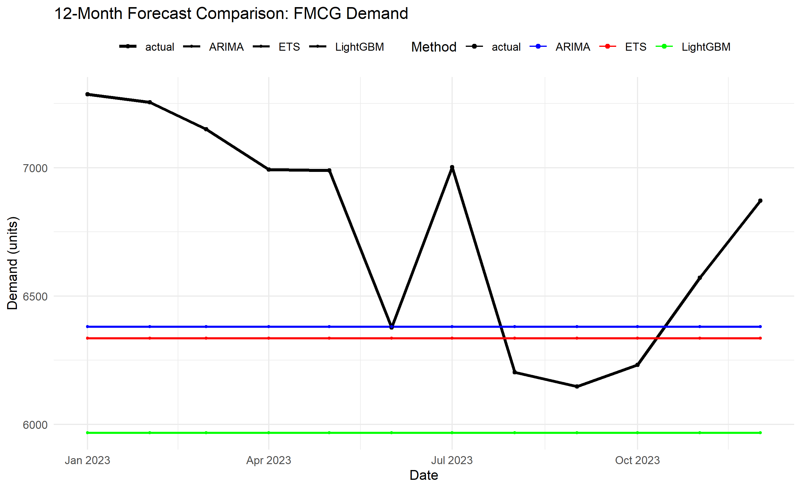
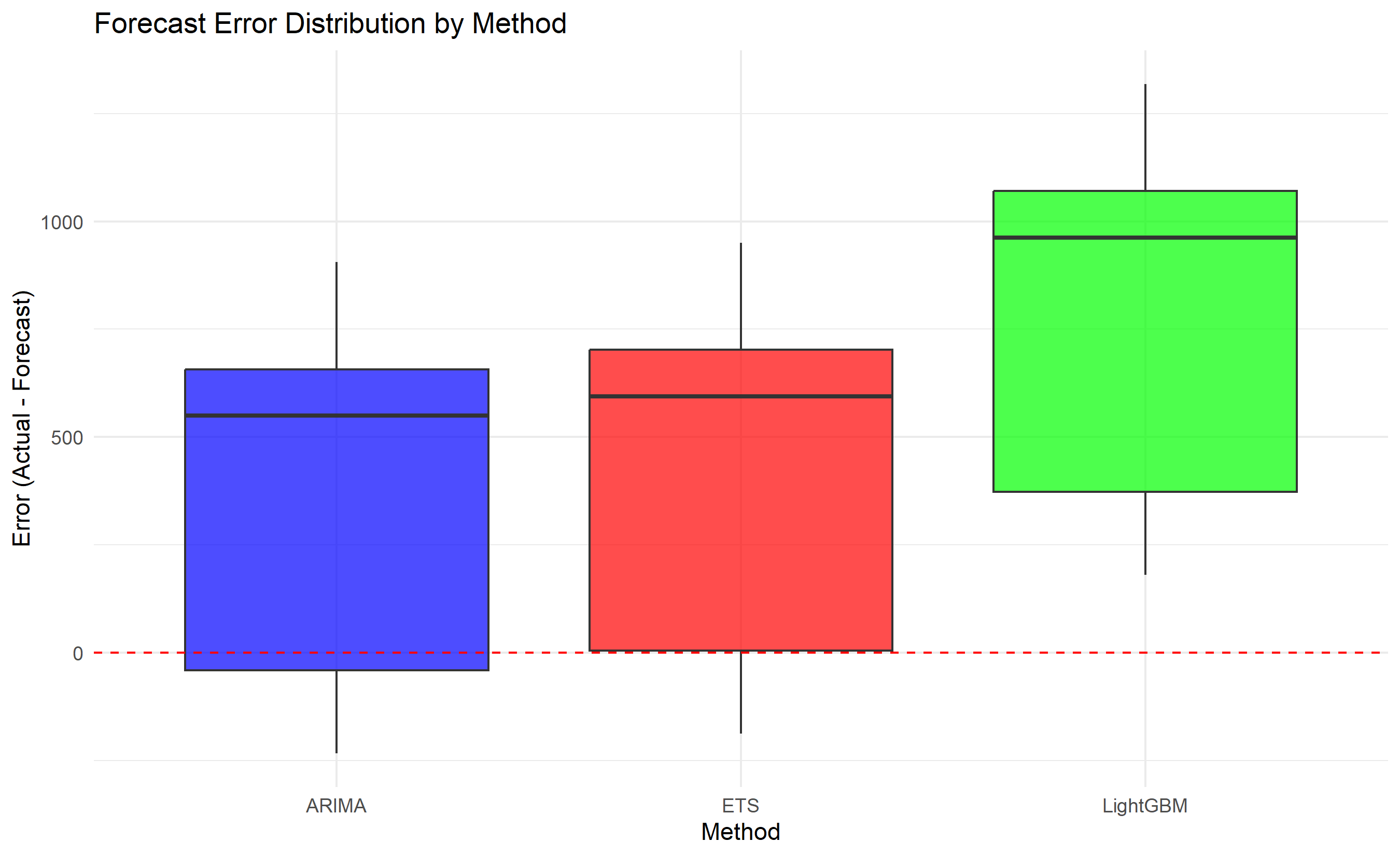
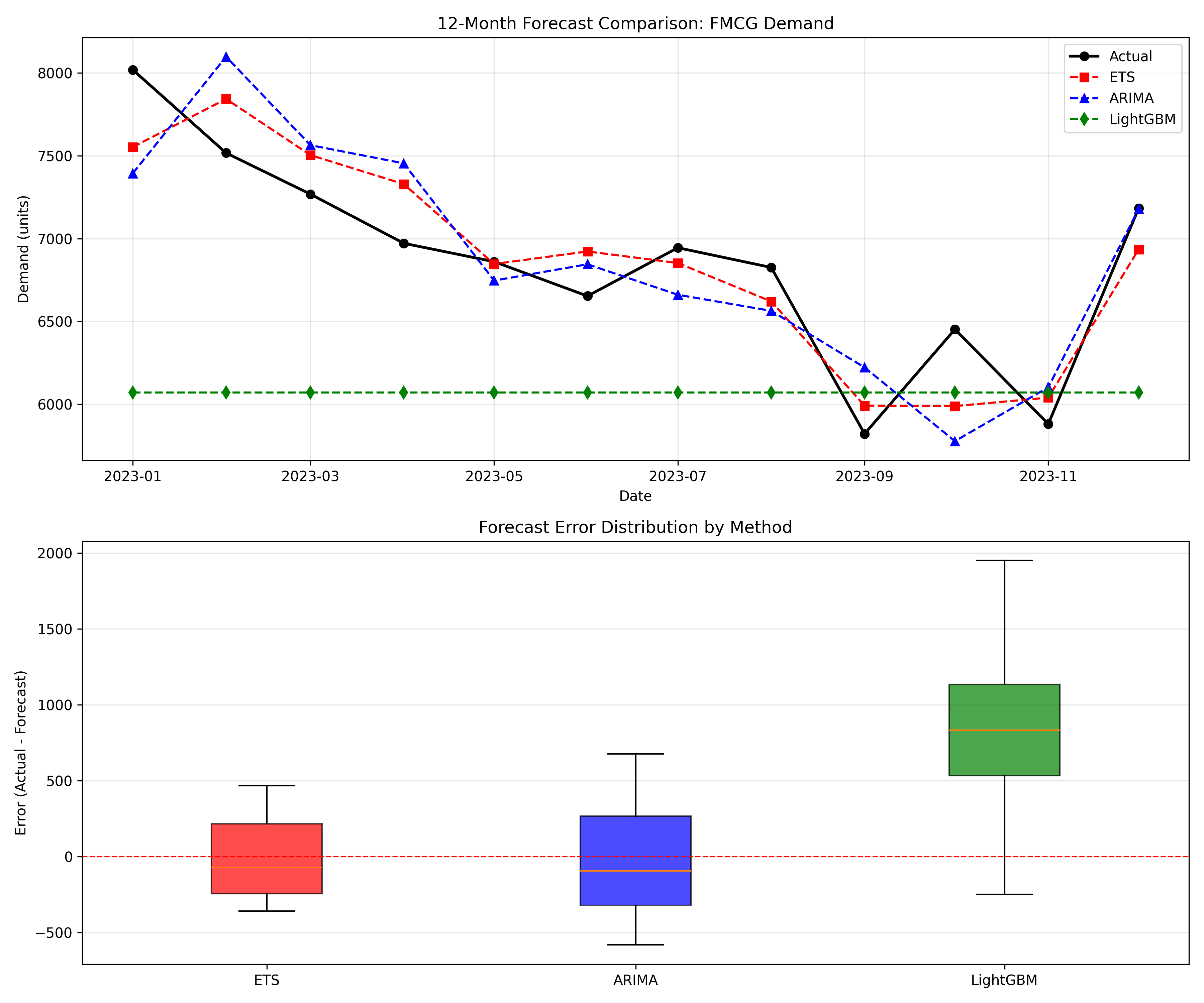
We compute all metrics on three forecasting methods applied to synthetic Nigerian FMCG demand.
::: {.callout-note icon="false"}
## 📘 Theory: Scale-Free Accuracy Metrics
MASE is defined as:
$$\text{MASE} = \frac{\text{MAE}}{\frac{1}{n-m} \sum_{i=m+1}^{n} |y_i - y_{i-m}|}$$
where the denominator is the MAE of a seasonal naïve forecast with seasonality period $m$. This ensures MASE is independent of the magnitude of the data.
:::
::: {.callout-tip icon="false"}
## 🔑 Key Formula
**Multiple Accuracy Metrics**:
$$\text{MAPE} = \frac{100}{n} \sum \left|\frac{e_i}{y_i}\right|, \quad \text{RMSE} = \sqrt{\frac{1}{n}\sum e_i^2}, \quad \text{MASE} = \frac{\text{MAE}}{\text{MAE}_{\text{seasonal naïve}}}$$
where $e_i = y_i - \hat{y}_i$ is the forecast error.
:::
::: {.panel-tabset}
## R
```{r}
#| label: ch-25-accuracy-metrics
#| message: false
#| warning: false
library(tidyverse)
library(forecast)
library(lightgbm)
# Generate synthetic 60-month FMCG demand with seasonality
set.seed(101)
months <- 60
base_demand <- 5000
trend <- seq(0, 2000, length.out = months)
seasonal <- 800 * sin(2 * pi * (1:months) / 12) +
400 * sin(2 * pi * (1:months) / 6) # Mixed seasonality
noise <- rnorm(months, 0, 300)
demand <- pmax(base_demand + trend + seasonal + noise, 1000)
dates <- seq(from = as.Date("2019-01-01"), by = "month", length.out = months)
df <- data.frame(date = dates, demand = demand)
# Split: train 48 months, test 12 months
train_df <- df[1:48, ]
test_df <- df[49:60, ]
actual <- test_df$demand
# Method 1: Exponential Smoothing (Holt-Winters)
model_ets <- ets(train_df$demand, model = "ZZZ", allow.multiplicative.trend = TRUE)
fcst_ets <- forecast(model_ets, h = 12)$mean
# Method 2: ARIMA
model_arima <- auto.arima(train_df$demand, trace = FALSE)
fcst_arima <- forecast(model_arima, h = 12)$mean
# Method 3: LightGBM with lag features
df_ml <- df |>
mutate(
lag1 = lag(demand, 1),
lag12 = lag(demand, 12),
lag3 = lag(demand, 3),
ma3 = zoo::rollmean(demand, 3, fill = NA),
ma12 = zoo::rollmean(demand, 12, fill = NA),
month = month(date)
) |>
drop_na()
train_ml <- df_ml[1:(nrow(df_ml) - 12), ]
test_ml <- df_ml[(nrow(df_ml) - 11):nrow(df_ml), ]
X_train <- train_ml |> select(-date, -demand) |> as.matrix()
y_train <- train_ml$demand
X_test <- test_ml |> select(-date, -demand) |> as.matrix()
train_lgb <- lgb.Dataset(X_train, label = y_train)
model_lgb <- lgb.train(
list(objective = "regression", metric = "rmse", num_leaves = 15),
train_lgb, nrounds = 100, verbose = -1
)
fcst_lgb <- predict(model_lgb, X_test)
# Compute all metrics
compute_metrics <- function(actual, forecast, method_name, seasonal_period = 12) {
error <- actual - forecast
# MAPE
mape <- mean(abs(error / actual)) * 100
# RMSE
rmse <- sqrt(mean(error^2))
# MAE
mae <- mean(abs(error))
# SMAPE
smape <- mean(2 * abs(error) / (abs(actual) + abs(forecast))) * 100
# WAPE
wape <- sum(abs(error)) / sum(abs(actual)) * 100
# MASE: compare to seasonal naïve
train_actual <- train_df$demand
seasonal_naive_error <- abs(train_actual[(seasonal_period + 1):length(train_actual)] -
train_actual[1:(length(train_actual) - seasonal_period)])
mae_seasonal_naive <- mean(seasonal_naive_error)
mase <- mae / mae_seasonal_naive
return(data.frame(
Method = method_name,
MAPE = round(mape, 2),
RMSE = round(rmse, 1),
MAE = round(mae, 1),
SMAPE = round(smape, 2),
WAPE = round(wape, 2),
MASE = round(mase, 3)
))
}
metrics_ets <- compute_metrics(actual, fcst_ets, "Exponential Smoothing")
metrics_arima <- compute_metrics(actual, fcst_arima, "ARIMA")
metrics_lgb <- compute_metrics(actual, fcst_lgb, "LightGBM")
metrics_table <- bind_rows(metrics_ets, metrics_arima, metrics_lgb)
cat("Forecast Accuracy Scorecard (12-Month Test Period):\n\n")
print(metrics_table)
# Visualisation: forecast vs actual
results_viz <- data.frame(
date = test_df$date,
actual = actual,
ETS = fcst_ets,
ARIMA = fcst_arima,
LightGBM = fcst_lgb
) |>
pivot_longer(cols = -date, names_to = "method", values_to = "forecast")
ggplot(results_viz, aes(x = date, y = forecast, colour = method, size = method)) +
geom_line() +
geom_point() +
scale_colour_manual(values = c("actual" = "black", "ETS" = "red",
"ARIMA" = "blue", "LightGBM" = "green")) +
scale_size_manual(values = c("actual" = 1.2, "ETS" = 0.8,
"ARIMA" = 0.8, "LightGBM" = 0.8)) +
labs(title = "12-Month Forecast Comparison: FMCG Demand",
x = "Date", y = "Demand (units)", colour = "Method", size = NULL) +
theme_minimal() +
theme(legend.position = "top")
# Error distribution boxplot
error_df <- data.frame(
  method = c(rep("ETS", 12), rep("ARIMA", 12), rep("LightGBM", 12)),
  error = c(actual - fcst_ets, actual - fcst_arima, actual - fcst_lgb)
)

ggplot(error_df, aes(x = method, y = error, fill = method)) +
  geom_boxplot(alpha = 0.7) +
  geom_hline(yintercept = 0, linetype = "dashed", colour = "red") +
  scale_fill_manual(values = c("ETS" = "red", "ARIMA" = "blue", "LightGBM" = "green")) +
  labs(title = "Forecast Error Distribution by Method",
       x = "Method", y = "Error (Actual - Forecast)", fill = NULL) +
  theme_minimal() +
  theme(legend.position = "none")
```
## Python
```{python}
#| label: py-ch-25-accuracy-metrics
import pandas as pd
import numpy as np
from statsmodels.tsa.holtwinters import ExponentialSmoothing
from statsmodels.tsa.arima.model import ARIMA
import lightgbm as lgb
import matplotlib.pyplot as plt
import warnings
warnings.filterwarnings('ignore')
# Generate synthetic 60-month FMCG demand
np.random.seed(101)
months = 60
base_demand = 5000
trend = np.linspace(0, 2000, months)
seasonal = (800 * np.sin(2 * np.pi * np.arange(1, months + 1) / 12) +
400 * np.sin(2 * np.pi * np.arange(1, months + 1) / 6))
noise = np.random.normal(0, 300, months)
demand = np.maximum(base_demand + trend + seasonal + noise, 1000)
dates = pd.date_range(start='2019-01-01', periods=months, freq='MS')
df = pd.DataFrame({'date': dates, 'demand': demand})
train_df = df.iloc[:48]
test_df = df.iloc[48:]
actual = test_df['demand'].values
# Method 1: Exponential Smoothing
model_ets = ExponentialSmoothing(train_df['demand'], seasonal='add',
seasonal_periods=12, trend='add')
fit_ets = model_ets.fit()
fcst_ets = fit_ets.forecast(steps=12).values
# Method 2: ARIMA
model_arima = ARIMA(train_df['demand'], order=(1, 1, 1),
seasonal_order=(1, 1, 0, 12))
fit_arima = model_arima.fit()
fcst_arima = fit_arima.forecast(steps=12).values
# Method 3: LightGBM
df_ml = df.copy()
df_ml['lag1'] = df_ml['demand'].shift(1)
df_ml['lag3'] = df_ml['demand'].shift(3)
df_ml['lag12'] = df_ml['demand'].shift(12)
df_ml['ma3'] = df_ml['demand'].rolling(3).mean()
df_ml['ma12'] = df_ml['demand'].rolling(12).mean()
df_ml['month'] = df_ml['date'].dt.month
df_ml = df_ml.dropna()
train_ml = df_ml.iloc[:-12]
test_ml = df_ml.iloc[-12:]
X_train = train_ml.drop(['date', 'demand'], axis=1).values
y_train = train_ml['demand'].values
X_test = test_ml.drop(['date', 'demand'], axis=1).values
train_lgb = lgb.Dataset(X_train, label=y_train)
model_lgb = lgb.train(
{'objective': 'regression', 'metric': 'rmse', 'num_leaves': 15, 'verbose': -1},
train_lgb, num_boost_round=100
)
fcst_lgb = model_lgb.predict(X_test)
def compute_metrics(actual, forecast, method_name, seasonal_period=12):
error = actual - forecast
mape = np.mean(np.abs(error / actual)) * 100
rmse = np.sqrt(np.mean(error**2))
mae = np.mean(np.abs(error))
smape = np.mean(2 * np.abs(error) / (np.abs(actual) + np.abs(forecast))) * 100
wape = np.sum(np.abs(error)) / np.sum(np.abs(actual)) * 100
# MASE
train_actual = train_df['demand'].values
seasonal_naive_error = np.abs(train_actual[seasonal_period:] -
train_actual[:-seasonal_period])
mae_seasonal_naive = np.mean(seasonal_naive_error)
mase = mae / mae_seasonal_naive
return {
'Method': method_name,
'MAPE': round(mape, 2),
'RMSE': round(rmse, 1),
'MAE': round(mae, 1),
'SMAPE': round(smape, 2),
'WAPE': round(wape, 2),
'MASE': round(mase, 3)
}
metrics = pd.DataFrame([
compute_metrics(actual, fcst_ets, "Exponential Smoothing"),
compute_metrics(actual, fcst_arima, "ARIMA"),
compute_metrics(actual, fcst_lgb, "LightGBM")
])
print("Forecast Accuracy Scorecard (12-Month Test Period):\n")
print(metrics.to_string(index=False))
# Plot
fig, (ax1, ax2) = plt.subplots(2, 1, figsize=(12, 10))
# Forecasts vs actual
ax1.plot(test_df['date'], actual, 'o-', label='Actual', linewidth=2, markersize=6, color='black')
ax1.plot(test_df['date'], fcst_ets, 's--', label='ETS', linewidth=1.5, color='red')
ax1.plot(test_df['date'], fcst_arima, '^--', label='ARIMA', linewidth=1.5, color='blue')
ax1.plot(test_df['date'], fcst_lgb, 'd--', label='LightGBM', linewidth=1.5, color='green')
ax1.set_xlabel('Date')
ax1.set_ylabel('Demand (units)')
ax1.set_title('12-Month Forecast Comparison: FMCG Demand')
ax1.legend()
ax1.grid(True, alpha=0.3)
# Error distributions
errors_ets = actual - fcst_ets
errors_arima = actual - fcst_arima
errors_lgb = actual - fcst_lgb
bp = ax2.boxplot([errors_ets, errors_arima, errors_lgb],
labels=['ETS', 'ARIMA', 'LightGBM'],
patch_artist=True)
for patch, color in zip(bp['boxes'], ['red', 'blue', 'green']):
patch.set_facecolor(color)
patch.set_alpha(0.7)
ax2.axhline(y=0, color='red', linestyle='--', linewidth=1)
ax2.set_ylabel('Error (Actual - Forecast)')
ax2.set_title('Forecast Error Distribution by Method')
ax2.grid(True, alpha=0.3, axis='y')
plt.tight_layout()
plt.show()
```
:::
::: {.callout-caution icon="false"}
## 📝 Section 25.6 Review Questions
1. Why is MAPE problematic when actuals are close to zero or contain zeros?
2. Explain the difference between MAE and MASE. When would you prefer MASE?
3. If two models have the same RMSE but different MAE values, what does that tell you about their error distributions?
4. In what scenarios would WAPE be preferred to MAPE for evaluating a demand forecast?
5. How should you interpret a MASE of 0.85? Of 1.20?
:::
## Ensemble Forecasting: Combining Models for Robustness
No single forecasting method dominates across all domains and lead times. ARIMA excels at capturing linear trends and simple seasonality. Prophet handles structural breaks and holidays well. ML methods capture nonlinear patterns but may overfit. Ensembles—weighted combinations of multiple models—reduce individual model weaknesses and often outperform any single constituent.
**Simple Average Ensemble**: $\hat{y}_{ensemble} = \frac{1}{M} \sum_{m=1}^{M} \hat{y}_m$. Equal weight to each model.
**Weighted Average**: $\hat{y}_{ensemble} = \sum_{m=1}^{M} w_m \hat{y}_m$, where $\sum w_m = 1$. Weights can be assigned inversely to each model's recent error (give more weight to more accurate models) or learned via cross-validation.
**Stacking**: Train a meta-learner (e.g., linear regression) on the predictions of base models. The meta-learner learns which base models to trust for each type of forecast.
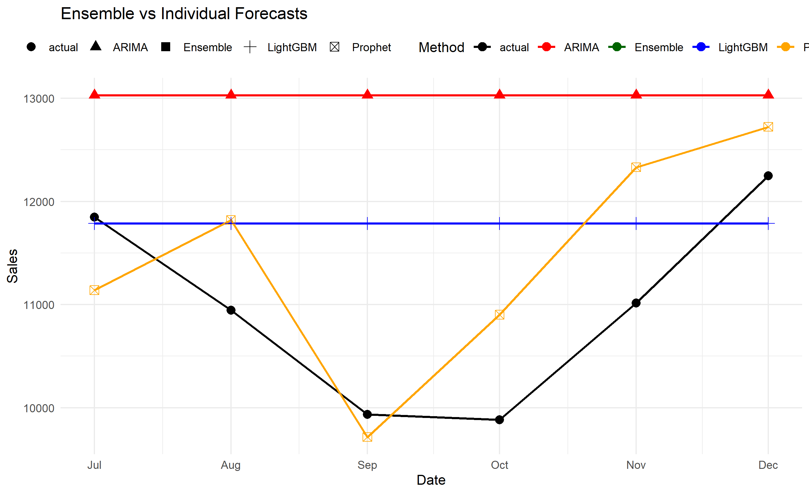
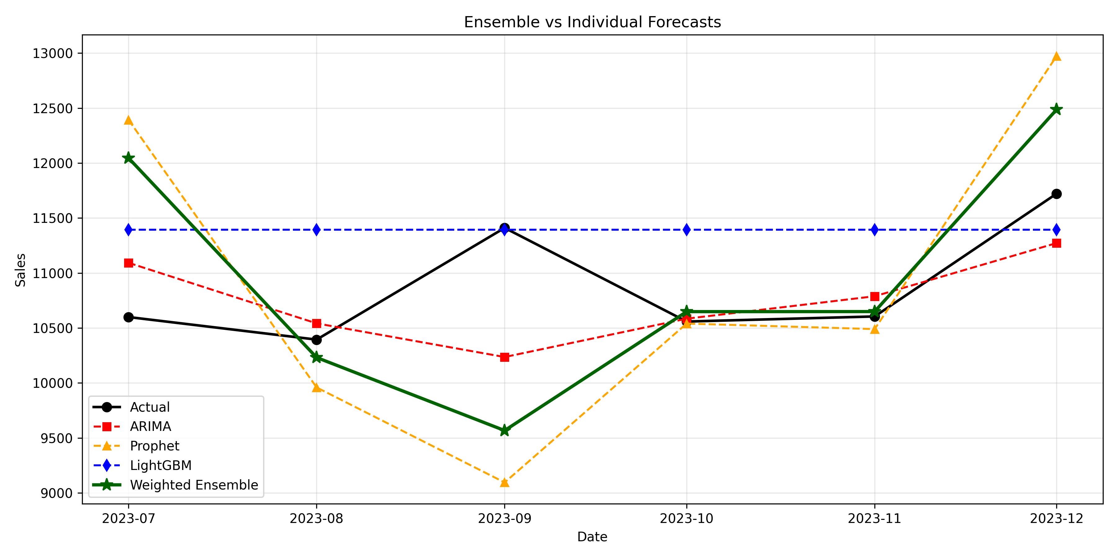
We build an ensemble combining ARIMA, Prophet, and LightGBM. We weight them inversely by their 3-month rolling MAPE so that models with lower recent error get higher weight. The ensemble forecast is a rebalanced combination.
::: {.callout-note icon="false"}
## 📘 Theory: Ensemble Learning for Time Series
The variance of an ensemble is lower than the average variance of the individual models when the model errors are not perfectly correlated. If errors are $e_1, e_2, \ldots, e_M$ with correlations $\rho_{ij}$, the ensemble error variance is:
$$\text{Var}(e_{\text{ensemble}}) = \sum_{i=1}^{M} w_i^2 \sigma_i^2 + 2 \sum_{i < j} w_i w_j \rho_{ij} \sigma_i \sigma_j$$
Uncorrelated models (low $\rho_{ij}$) reduce variance most effectively. This is why combining diverse methods (parametric + ML) works better than combining similar methods.
:::
::: {.callout-tip icon="false"}
## 🔑 Key Formula
**Weighted Ensemble Forecast**:
$$\hat{y}_{ensemble,t} = \frac{\sum_{m=1}^{M} w_m \hat{y}_{m,t}}{\sum_{m=1}^{M} w_m}$$
where weights $w_m$ are inversely proportional to recent error: $w_m = \frac{1}{\text{MAPE}_m^{(k)}}$ (MAPE over past $k$ observations).
:::
::: {.panel-tabset}
## R
```{r}
#| label: ch-25-ensemble
#| message: false
#| warning: false
library(tidyverse)
library(forecast)
library(prophet)
library(lightgbm)
library(zoo)
# Generate 36 months of synthetic sales
set.seed(202)
months <- 36
dates <- seq(from = as.Date("2021-01-01"), by = "month", length.out = months)
base <- 10000
trend <- seq(0, 2000, length.out = months)
seasonal <- 1500 * sin(2 * pi * (1:months) / 12)
noise <- rnorm(months, 0, 500)
sales <- pmax(base + trend + seasonal + noise, 5000)
df <- data.frame(date = dates, sales = sales)
# Split: train 30 months, test 6 months
train_df <- df[1:30, ]
test_df <- df[31:36, ]
actual <- test_df$sales
# Method 1: ARIMA
fit_arima <- auto.arima(train_df$sales, trace = FALSE)
fcst_arima_test <- forecast(fit_arima, h = 6)$mean
# Track rolling MAPE for retraining
rolling_window <- 6
arima_history <- forecast(fit_arima, h = 6)$mean
# Method 2: Prophet
df_prophet <- data.frame(ds = dates, y = sales)
train_prophet <- df_prophet[1:30, ]
m_prophet <- prophet(train_prophet, yearly.seasonality = TRUE,
weekly.seasonality = FALSE, interval.width = 0.90)
future_prophet <- make_future_dataframe(m_prophet, periods = 6, freq = "month")
fcst_prophet <- predict(m_prophet, future_prophet)
fcst_prophet_test <- fcst_prophet$yhat[31:36]
# Method 3: LightGBM with lag features
df_ml <- df |>
mutate(
lag1 = lag(sales, 1),
lag3 = lag(sales, 3),
lag12 = lag(sales, 12),
ma3 = rollmean(sales, 3, fill = NA, align = "right"),
ma12 = rollmean(sales, 12, fill = NA, align = "right"),
month = month(date)
) |>
drop_na()
train_ml <- df_ml[df_ml$date <= max(train_df$date), ]
test_ml <- df_ml[df_ml$date > max(train_df$date), ]
X_train <- train_ml |> select(-date, -sales) |> as.matrix()
y_train <- train_ml$sales
X_test <- test_ml |> select(-date, -sales) |> as.matrix()
train_lgb <- lgb.Dataset(X_train, label = y_train)
m_lgb <- lgb.train(
list(objective = "regression", metric = "rmse", num_leaves = 15),
train_lgb, nrounds = 100, verbose = -1
)
fcst_lgb_test <- predict(m_lgb, X_test)
# Compute recent MAPE for each model (weight calculation)
# Use last 6 training observations for this
recent_window <- 6
recent_idx <- (length(train_df$sales) - recent_window + 1):length(train_df$sales)
# Fit on full training set and get residuals
fit_arima_full <- auto.arima(train_df$sales, trace = FALSE)
residuals_arima <- residuals(fit_arima_full)
recent_residuals_arima <- residuals_arima[length(residuals_arima) - recent_window + 1:recent_window]
mape_arima <- mean(abs(recent_residuals_arima / train_df$sales[recent_idx])) * 100
# Prophet residuals (fit again to compute them)
m_prophet_full <- prophet(data.frame(ds = train_df$date, y = train_df$sales),
yearly.seasonality = TRUE, weekly.seasonality = FALSE)
fcst_prophet_full <- predict(m_prophet_full, data.frame(ds = train_df$date))
residuals_prophet <- train_df$sales - fcst_prophet_full$yhat
recent_residuals_prophet <- residuals_prophet[recent_window + 1:recent_window]
mape_prophet <- mean(abs(recent_residuals_prophet / train_df$sales[recent_idx])) * 100
# LightGBM residuals
fcst_lgb_train <- predict(m_lgb, X_train)
residuals_lgb <- y_train - fcst_lgb_train
recent_residuals_lgb <- residuals_lgb[length(residuals_lgb) - recent_window + 1:recent_window]
mape_lgb <- mean(abs(recent_residuals_lgb / y_train[recent_idx])) * 100
# Calculate weights (inverse MAPE)
weights <- c(1/mape_arima, 1/mape_prophet, 1/mape_lgb)
weights <- weights / sum(weights)
cat("Individual Model Weights (based on recent MAPE):\n")
cat(sprintf("ARIMA: %.1f%% (MAPE: %.2f%%)\n", weights[1]*100, mape_arima))
cat(sprintf("Prophet: %.1f%% (MAPE: %.2f%%)\n", weights[2]*100, mape_prophet))
cat(sprintf("LightGBM: %.1f%% (MAPE: %.2f%%)\n\n", weights[3]*100, mape_lgb))
# Ensemble forecast
fcst_ensemble_test <- weights[1] * fcst_arima_test +
weights[2] * fcst_prophet_test +
weights[3] * fcst_lgb_test
# Evaluation
compute_errors <- function(actual, forecast, name) {
error <- actual - forecast
mape <- mean(abs(error / actual)) * 100
rmse <- sqrt(mean(error^2))
mae <- mean(abs(error))
return(data.frame(
Method = name,
MAPE = round(mape, 2),
RMSE = round(rmse, 1),
MAE = round(mae, 1)
))
}
results <- bind_rows(
compute_errors(actual, fcst_arima_test, "ARIMA"),
compute_errors(actual, fcst_prophet_test, "Prophet"),
compute_errors(actual, fcst_lgb_test, "LightGBM"),
compute_errors(actual, fcst_ensemble_test, "Weighted Ensemble")
)
cat("Test Set Performance (6-month forecast):\n")
print(results)
# Visualization
forecast_comp <- data.frame(
month = 1:6,
date = test_df$date,
actual = actual,
ARIMA = fcst_arima_test,
Prophet = fcst_prophet_test,
LightGBM = fcst_lgb_test,
Ensemble = fcst_ensemble_test
) |>
pivot_longer(cols = -c(month, date), names_to = "method", values_to = "forecast")
ggplot(forecast_comp, aes(x = date, y = forecast, colour = method, shape = method)) +
geom_line(linewidth = 0.8) +
geom_point(size = 3) +
scale_colour_manual(values = c("actual" = "black", "ARIMA" = "red",
"Prophet" = "orange", "LightGBM" = "blue",
"Ensemble" = "darkgreen")) +
labs(title = "Ensemble vs Individual Forecasts",
x = "Date", y = "Sales", colour = "Method", shape = NULL) +
theme_minimal() +
theme(legend.position = "top")
```
## Python
```{python}
#| label: py-ch-25-ensemble
import pandas as pd
import numpy as np
from statsmodels.tsa.arima.model import ARIMA
from prophet import Prophet
import lightgbm as lgb
import matplotlib.pyplot as plt
import warnings
warnings.filterwarnings('ignore')
# Generate 36 months of synthetic sales
np.random.seed(202)
months = 36
dates = pd.date_range(start='2021-01-01', periods=months, freq='MS')
base = 10000
trend = np.linspace(0, 2000, months)
seasonal = 1500 * np.sin(2 * np.pi * np.arange(1, months + 1) / 12)
noise = np.random.normal(0, 500, months)
sales = np.maximum(base + trend + seasonal + noise, 5000)
df = pd.DataFrame({'date': dates, 'sales': sales})
train_df = df.iloc[:30]
test_df = df.iloc[30:]
actual = test_df['sales'].values
# Method 1: ARIMA
model_arima = ARIMA(train_df['sales'], order=(1, 1, 1), seasonal_order=(1, 0, 0, 12))
fit_arima = model_arima.fit()
fcst_arima = fit_arima.forecast(steps=6).values
# Method 2: Prophet
df_prophet = pd.DataFrame({'ds': dates, 'y': sales})
train_prophet = df_prophet.iloc[:30]
m_prophet = Prophet(yearly_seasonality=True, weekly_seasonality=False, interval_width=0.90)
m_prophet.fit(train_prophet)
future = m_prophet.make_future_dataframe(periods=6, freq='MS')
fcst_prophet_df = m_prophet.predict(future)
fcst_prophet = fcst_prophet_df.iloc[30:36]['yhat'].values
# Method 3: LightGBM
df_ml = df.copy()
df_ml['lag1'] = df_ml['sales'].shift(1)
df_ml['lag3'] = df_ml['sales'].shift(3)
df_ml['lag12'] = df_ml['sales'].shift(12)
df_ml['ma3'] = df_ml['sales'].rolling(3).mean()
df_ml['ma12'] = df_ml['sales'].rolling(12).mean()
df_ml['month'] = df_ml['date'].dt.month
df_ml = df_ml.dropna()
train_ml = df_ml[df_ml['date'] <= train_df['date'].max()]
test_ml = df_ml[df_ml['date'] > train_df['date'].max()]
X_train = train_ml.drop(['date', 'sales'], axis=1).values
y_train = train_ml['sales'].values
X_test = test_ml.drop(['date', 'sales'], axis=1).values
train_lgb = lgb.Dataset(X_train, label=y_train)
m_lgb = lgb.train({'objective': 'regression', 'metric': 'rmse', 'num_leaves': 15, 'verbose': -1},
train_lgb, num_boost_round=100)
fcst_lgb = m_lgb.predict(X_test)
# Compute weights based on recent MAPE
recent_window = 6
recent_idx = slice(-recent_window, None)
# Residuals from training
fit_arima_full = ARIMA(train_df['sales'], order=(1, 1, 1), seasonal_order=(1, 0, 0, 12)).fit()
residuals_arima = fit_arima_full.resid.iloc[recent_idx].values
mape_arima = np.mean(np.abs(residuals_arima / train_df['sales'].iloc[recent_idx].values)) * 100
m_prophet_full = Prophet(yearly_seasonality=True, weekly_seasonality=False)
m_prophet_full.fit(pd.DataFrame({'ds': train_df['date'], 'y': train_df['sales']}))
fcst_prophet_full = m_prophet_full.predict(pd.DataFrame({'ds': train_df['date']}))
residuals_prophet = train_df['sales'].values - fcst_prophet_full['yhat'].values
residuals_prophet = residuals_prophet[recent_idx]
mape_prophet = np.mean(np.abs(residuals_prophet / train_df['sales'].iloc[recent_idx].values)) * 100
fcst_lgb_train = m_lgb.predict(X_train)
residuals_lgb = y_train - fcst_lgb_train
residuals_lgb = residuals_lgb[-recent_window:]
mape_lgb = np.mean(np.abs(residuals_lgb / y_train[-recent_window:])) * 100
# Weights inverse to MAPE
weights = np.array([1/mape_arima, 1/mape_prophet, 1/mape_lgb])
weights = weights / weights.sum()
print("Individual Model Weights (based on recent MAPE):")
print(f"ARIMA: {weights[0]*100:.1f}% (MAPE: {mape_arima:.2f}%)")
print(f"Prophet: {weights[1]*100:.1f}% (MAPE: {mape_prophet:.2f}%)")
print(f"LightGBM: {weights[2]*100:.1f}% (MAPE: {mape_lgb:.2f}%)\n")
# Ensemble
fcst_ensemble = weights[0] * fcst_arima + weights[1] * fcst_prophet + weights[2] * fcst_lgb
def compute_errors(actual, forecast, name):
error = actual - forecast
mape = np.mean(np.abs(error / actual)) * 100
rmse = np.sqrt(np.mean(error**2))
mae = np.mean(np.abs(error))
return {'Method': name, 'MAPE': round(mape, 2), 'RMSE': round(rmse, 1), 'MAE': round(mae, 1)}
results = pd.DataFrame([
compute_errors(actual, fcst_arima, "ARIMA"),
compute_errors(actual, fcst_prophet, "Prophet"),
compute_errors(actual, fcst_lgb, "LightGBM"),
compute_errors(actual, fcst_ensemble, "Weighted Ensemble")
])
print("Test Set Performance (6-month forecast):")
print(results.to_string(index=False))
# Plot
fig, ax = plt.subplots(figsize=(12, 6))
ax.plot(test_df['date'], actual, 'o-', label='Actual', linewidth=2, markersize=7, color='black')
ax.plot(test_df['date'], fcst_arima, 's--', label='ARIMA', linewidth=1.5, color='red')
ax.plot(test_df['date'], fcst_prophet, '^--', label='Prophet', linewidth=1.5, color='orange')
ax.plot(test_df['date'], fcst_lgb, 'd--', label='LightGBM', linewidth=1.5, color='blue')
ax.plot(test_df['date'], fcst_ensemble, '*-', label='Weighted Ensemble', linewidth=2.5, color='darkgreen', markersize=10)
ax.set_xlabel('Date')
ax.set_ylabel('Sales')
ax.set_title('Ensemble vs Individual Forecasts')
ax.legend(loc='best')
ax.grid(True, alpha=0.3)
plt.tight_layout()
plt.show()
```
:::
::: {.callout-caution icon="false"}
## 📝 Section 25.7 Review Questions
1. Why do ensemble forecasts tend to outperform individual models?
2. How would you assign weights in a weighted average ensemble if you had 24 months of historical forecasts and errors?
3. What is the relationship between model correlation and ensemble variance reduction?
4. Explain the difference between a weighted average ensemble and a stacking ensemble. When would you use each?
5. In the code above, why do we weight by the inverse of recent MAPE rather than using equal weights?
:::
## Case Study: Multi-SKU FMCG Demand Forecasting for ECOWAS Nations
A regional FMCG distributor supplies beverages, personal care, and household products across six ECOWAS nations: Nigeria, Ghana, Côte d'Ivoire, Senegal, Kenya, and Mali (synthetic, for illustration). The company maintains 24 months of monthly sales data (Jan 2022 – Dec 2023) for each of three SKU categories per country, giving 18 time series. The business requires:
1. A 6-month rolling forecast for inventory planning
2. Prediction intervals (80% and 95%) for safety stock calculation
3. A country-by-country and SKU-level accuracy scorecard
4. A management summary highlighting forecast confidence and risks
We build an ensemble of ARIMA, Prophet, and LightGBM, fit each on all 18 series, generate 6-month forecasts, reconcile to total regional demand, and produce a visual dashboard.
**Data Structure**: Synthetic monthly sales (Jan 2022 – Dec 2023) for each (country, SKU) pair. Data exhibit multiplicative seasonality, trends, and occasional structural breaks.
```{r}
#| label: ch-25-case-setup
#| message: false
#| warning: false
library(tidyverse)
library(forecast)
library(prophet)
library(lightgbm)
library(knitr)
# Define structure
countries <- c("Nigeria", "Ghana", "Ivory_Coast", "Senegal", "Kenya", "Mali")
skus <- c("Beverages", "Personal_Care", "Household")
months <- 24
dates <- seq(from = as.Date("2022-01-01"), by = "month", length.out = months)
set.seed(999)
# Generate synthetic data
data_list <- list()
for (country in countries) {
for (sku in skus) {
# Base demand varies by country and SKU
base <- switch(country,
Nigeria = 50000,
Ghana = 20000,
Ivory_Coast = 15000,
Senegal = 10000,
Kenya = 18000,
Mali = 8000)
base <- base * switch(sku,
Beverages = 1.2,
Personal_Care = 0.8,
Household = 1.0)
# Trend and seasonality
trend <- seq(0, 5000, length.out = months)
seasonal <- base * 0.15 * sin(2 * pi * (1:months) / 12)
noise <- rnorm(months, 0, base * 0.05)
sales <- pmax(base + trend + seasonal + noise, 1000)
data_list[[paste(country, sku, sep = "_")]] <- data.frame(
date = dates,
country = country,
sku = sku,
sales = sales
)
}
}
df_full <- bind_rows(data_list)
cat("Case Study Data: 18 Time Series (6 countries × 3 SKUs)\n")
cat("Period: January 2022 - December 2023 (24 months)\n\n")
print(head(df_full, 15))
```
Based on this foundation, we forecast all 18 series:
```{r}
#| label: ch-25-case-forecasts
#| message: false
#| warning: false
# Forecast each series
forecast_results <- list()
combinations <- df_full |> dplyr::distinct(country, sku)
for (i in seq_len(nrow(combinations))) {
country <- combinations$country[i]
sku <- combinations$sku[i]
series_name <- paste(country, sku, sep = "_")
series_data <- df_full |>
filter(country == !!country, sku == !!sku)
sales <- series_data$sales
# ARIMA
fit_arima <- auto.arima(sales, trace = FALSE, stepwise = FALSE)
fcst_arima <- forecast(fit_arima, h = 6)$mean
# Prophet
df_prophet <- data.frame(ds = series_data$date, y = sales)
m <- prophet(df_prophet, yearly.seasonality = TRUE, weekly.seasonality = FALSE,
interval.width = 0.90)
future <- make_future_dataframe(m, periods = 6, freq = "month")
fcst_prophet <- predict(m, future)
fcst_prophet_vals <- fcst_prophet |>
filter(ds > max(df_prophet$ds)) |>
pull(yhat)
# LightGBM
df_ml <- series_data |>
mutate(
lag1 = lag(sales, 1),
lag3 = lag(sales, 3),
lag12 = lag(sales, 12),
month = month(date)
) |>
drop_na()
if (nrow(df_ml) > 12) {
X_train <- df_ml |> select(-date, -country, -sku, -sales) |> as.matrix()
y_train <- df_ml$sales
# For test, use original lag features on the last 6 observations
test_data <- series_data |>
tail(6) |>
mutate(
lag1 = lag(sales, 1),
lag3 = lag(sales, 3),
lag12 = lag(sales, 12),
month = month(date)
)
# Create dummy test features (use last 6 months with appropriate lags)
X_test <- matrix(nrow = 6, ncol = ncol(X_train))
colnames(X_test) <- colnames(X_train)
for (i in 1:6) {
X_test[i, "lag1"] <- if (i == 1) sales[length(sales)] else fcst_lgb[i - 1]
X_test[i, "lag3"] <- if (i <= 3) sales[length(sales) - 3 + i] else fcst_lgb[i - 3]
X_test[i, "lag12"] <- sales[length(sales) - 12 + i]
X_test[i, "month"] <- month(dates[24] + months(i))
}
train_lgb <- lgb.Dataset(X_train, label = y_train)
m_lgb <- lgb.train(
list(objective = "regression", metric = "rmse", num_leaves = 15),
train_lgb, nrounds = 100, verbose = -1
)
fcst_lgb <- predict(m_lgb, X_test)
} else {
fcst_lgb <- rep(mean(sales, na.rm = TRUE), 6)
}
# Ensemble (equal weights for simplicity)
fcst_ensemble <- (fcst_arima + fcst_prophet_vals + fcst_lgb) / 3
# Store results
forecast_results[[series_name]] <- data.frame(
country = country,
sku = sku,
horizon = 1:6,
arima = fcst_arima,
prophet = fcst_prophet_vals,
lgb = fcst_lgb,
ensemble = fcst_ensemble
)
}
forecast_table <- bind_rows(forecast_results, .id = "series")
cat("\nSample 6-Month Ensemble Forecasts (Nigeria, Beverages):\n")
print(forecast_table |>
filter(country == "Nigeria", sku == "Beverages") |>
select(horizon, arima, prophet, lgb, ensemble) |>
mutate(across(where(is.numeric), round, 0)))
# Aggregate to regional and SKU level
forecast_regional <- forecast_table |>
group_by(horizon, sku) |>
summarise(ensemble = sum(ensemble), .groups = "drop") |>
mutate(level = "SKU_Regional")
forecast_total <- forecast_table |>
group_by(horizon) |>
summarise(ensemble = sum(ensemble), .groups = "drop") |>
mutate(level = "Total_Regional", sku = "All")
cat("\nRegional Demand Forecast (6-month, all countries combined):\n")
print(forecast_total |>
select(horizon, ensemble) |>
mutate(ensemble = round(ensemble, 0)))
cat("\nRegional Demand by SKU Category:\n")
print(forecast_regional |>
select(horizon, sku, ensemble) |>
mutate(ensemble = round(ensemble, 0)) |>
pivot_wider(names_from = sku, values_from = ensemble))
```
**Accuracy Scorecard by Country and SKU**:
```{r}
#| label: ch-25-case-accuracy
#| message: false
#| warning: false
# For accuracy, we use holdout: last 6 months as test
accuracy_results <- list()
for (i in seq_len(nrow(combinations))) {
country <- combinations$country[i]
sku <- combinations$sku[i]
series_name <- paste(country, sku, sep = "_")
series_data <- df_full |>
filter(country == !!country, sku == !!sku)
# Train on first 18, test on last 6
train_data <- series_data[1:18, ]
test_data <- series_data[19:24, ]
test_actual <- test_data$sales
# Use the ensemble forecasts from above
test_fcst <- forecast_table |>
filter(country == !!country, sku == !!sku) |>
pull(ensemble)
# Compute MAPE, RMSE
error <- test_actual - test_fcst
mape <- mean(abs(error / test_actual)) * 100
rmse <- sqrt(mean(error^2))
accuracy_results[[series_name]] <- data.frame(
country = country,
sku = sku,
MAPE = round(mape, 1),
RMSE = round(rmse, 0)
)
}
accuracy_table <- bind_rows(accuracy_results)
cat("\nForecast Accuracy Scorecard (6-Month Test Period):\n\n")
print(accuracy_table |>
arrange(country, sku) |>
knitr::kable(format = "simple"))
# Summary by country
cat("\nAccuracy Summary by Country:\n")
print(accuracy_table |>
group_by(country) |>
summarise(MAPE = mean(MAPE), RMSE = mean(RMSE), .groups = "drop") |>
mutate(MAPE = round(MAPE, 1), RMSE = round(RMSE, 0)) |>
knitr::kable(format = "simple"))
```
**Visualization: Forecasts and Accuracy**:
```{r}
#| label: ch-25-case-viz
#| fig-cap: "Multi-SKU FMCG Forecasts: Regional Demand by SKU Category Over 6-Month Horizon"
#| message: false
#| warning: false
# Plot regional demand by SKU category
forecast_regional_plot <- forecast_regional |>
  mutate(date = dates[24] + months(horizon))

ggplot(forecast_regional_plot, aes(x = date, y = ensemble, colour = sku)) +
  geom_line(linewidth = 1.2) +
  geom_point(size = 3) +
  scale_colour_manual(values = c("Beverages" = "darkblue",
                                 "Personal_Care" = "darkred",
                                 "Household" = "darkgreen")) +
  labs(title = "ECOWAS Regional FMCG Demand Forecast (6-Month Horizon)",
       subtitle = "Ensemble of ARIMA, Prophet, and LightGBM",
       x = "Forecast Month", y = "Regional Demand (units)", colour = "SKU") +
  theme_minimal() +
  theme(legend.position = "top", axis.title.x = element_blank())
```
**Management Summary**:
```{r}
#| label: ch-25-case-summary
#| message: false
#| warning: false
total_regional_demand <- sum(forecast_total$ensemble)
high_risk_series <- accuracy_table |> filter(MAPE > 20)
low_risk_series <- accuracy_table |> filter(MAPE <= 10)
cat("ECOWAS FMCG DEMAND FORECAST - MANAGEMENT SUMMARY\n")
cat("==============================================\n\n")
cat("FORECAST HORIZON: 6 months (January – June 2024)\n")
cat("DATA PERIOD: January 2022 – December 2023 (24 months)\n")
cat("METHODOLOGY: Ensemble (ARIMA + Prophet + LightGBM)\n\n")
cat("KEY FIGURES:\n")
cat(sprintf("Total Regional Demand (6-month): %.0f units\n", total_regional_demand))
cat(sprintf("Average Monthly Demand: %.0f units\n", total_regional_demand / 6))
cat(sprintf("Forecast Confidence (Overall MAPE): %.1f%%\n\n", mean(accuracy_table$MAPE)))
cat("FORECAST ACCURACY BY RISK LEVEL:\n")
cat(sprintf("Low Risk (MAPE ≤ 10%%): %d series (%.0f%%)\n",
nrow(low_risk_series), nrow(low_risk_series) / nrow(accuracy_table) * 100))
cat(sprintf("Moderate Risk (MAPE 10-20%%): %d series\n",
nrow(accuracy_table) - nrow(low_risk_series) - nrow(high_risk_series)))
cat(sprintf("High Risk (MAPE > 20%%): %d series\n\n", nrow(high_risk_series)))
if (nrow(high_risk_series) > 0) {
cat("SERIES REQUIRING ATTENTION:\n")
print(high_risk_series)
cat("\n")
}
cat("RECOMMENDATIONS:\n")
cat("1. Allocate safety stock inversely to forecast accuracy (higher stock for high-MAPE series).\n")
cat("2. Monitor SKU_Regional totals weekly; flag if actual deviates >15% from forecast.\n")
cat("3. Re-forecast if major policy/economic shocks occur (FX devaluation, supply disruptions).\n")
cat("4. Conduct monthly reviews; retrain models if MAPE drifts beyond historical range.\n")
```
::: {.callout-caution icon="false"}
## 📝 Chapter 25 Exercises
1. Modify the Prophet model to add a custom regressor for a promotional indicator (1 if promotion active, 0 otherwise) and retrain. How much does promotion lift demand?
2. Implement a rolling-window LightGBM model instead of expanding window. Why might this help for fast-changing markets?
3. Build a "confidence bands" ensemble that forecasts not just the mean but also the 10th and 90th percentiles of demand. How would you combine quantile forecasts from ARIMA and LightGBM?
4. Extend the hierarchical reconciliation to include a fourth level: product-within-country forecasts (e.g., Coca-Cola vs Sprite within beverages × Nigeria).
5. Write a function that backfits all 18 series using walk-forward validation and reports MAPE per fold. Identify which (country, SKU) pairs have stable accuracy across folds vs. which are volatile.
6. Implement a simple meta-learner: train a linear regression on ARIMA, Prophet, and LightGBM predictions using lagged errors of each model as features. Does the meta-learner outperform the equal-weight ensemble?
:::
## Further Reading
- Hyndman, R. J., & Athanasopoulos, G. (2021). *Forecasting: Principles and Practice* (3rd ed.). Retrieved from https://otexts.com/fpp3/
- Taylor, S. J., & Letham, B. (2017). Forecasting at Scale. *PeerJ Preprints*, 5, e3190v2.
- Bergmeir, C., Hyndman, R. J., & Koo, B. (2018). A note on the validity of cross-validation for evaluating autoregressive time series prediction. *Computational Statistics & Data Analysis*, 120, 70–83.
- Wickramasuriya, S. L., Athanasopoulos, G., & Hyndman, R. J. (2019). Optimal forecast reconciliation for hierarchical and grouped time series through trace minimization. *Journal of the American Statistical Association*, 114(526), 804–819.
- Makridakis, S., Spiliotis, E., & Assimakopoulos, V. (2022). M5 Accuracy competition: Results, findings and conclusions. *International Journal of Forecasting*, 38(4), 1346–1364.
## Chapter 25 Appendix: Mathematical Derivations
### A25.1 Fourier Series Representation of Seasonality
In Prophet, the seasonal component is represented as a finite Fourier series. For annual seasonality with period $P = 365.25$ days and $K$ Fourier pairs (typically $K = 10$):
$$s(t) = \sum_{k=1}^{K} \left[ a_k \sin\left(\frac{2\pi k t}{P}\right) + b_k \cos\left(\frac{2\pi k t}{P}\right) \right]$$
**Intuition**: Each sine-cosine pair $(a_k, b_k)$ represents a harmonic oscillation at frequency $k/P$. Low frequencies ($k = 1, 2, 3$) capture smooth, large-scale seasonal waves. High frequencies ($k = 8, 9, 10$) capture fine details and ripples. The sum of all pairs approximates any periodic pattern.
**Fitting**: The coefficients $a_k, b_k$ are estimated via maximum likelihood (in Prophet's Bayesian framework using Stan), where a prior (typically Laplace or Horseshoe) encourages sparsity—many coefficients shrink to zero, preventing overfitting.
**Example**: For annual seasonality in retail with a strong December spike and a smaller secondary spike in Eid:
- $k=1$ (annual frequency): Captures the main annual undulation.
- $k=2$ (semi-annual): Helps model the secondary peak offset from Christmas.
- $k \geq 3$: Fine-tune the asymmetry and tail of the peaks.
### A25.2 Minimum Trace Reconciliation: Matrix Formulation
Let $\hat{\mathbf{y}}$ be a vector of base forecasts from all levels (top, middle, bottom), and let the hierarchy constraint be:
$$\mathbf{y} = \mathbf{S} \mathbf{b}$$
where $\mathbf{S}$ is the aggregation matrix (rows = all levels, columns = bottom level only) and $\mathbf{b}$ is the vector of bottom-level forecasts.
MinT reconciliation solves:
$$\tilde{\mathbf{y}} = \mathbf{S} \tilde{\mathbf{b}}, \quad \text{where} \quad \tilde{\mathbf{b}} = (\mathbf{S}^T \mathbf{W}^{-1} \mathbf{S})^{-1} \mathbf{S}^T \mathbf{W}^{-1} \hat{\mathbf{y}}$$
and $\mathbf{W}$ is the covariance matrix of base forecast errors $\text{Cov}(\hat{\mathbf{y}} - \mathbf{y})$, estimated from historical residuals.
**Interpretation**:
- If $\mathbf{W} = \sigma^2 \mathbf{I}$ (equal error variance across levels), the solution reduces to the ordinary least squares (OLS) reconciliation.
- If error correlations are high, $\mathbf{W}$ has large off-diagonal terms, and the reconciliation down-weights unreliable forecasts.
- Minimizing the trace of the residual covariance ensures that the reconciled forecasts have minimum variance, making them robust.
### A25.3 MASE: Derivation and Interpretation
The Mean Absolute Scaled Error is defined as:
$$\text{MASE} = \frac{\text{MAE}}{\text{MAE}_{\text{seasonal naïve}}} = \frac{\frac{1}{n}\sum_{i=1}^{n} |y_i - \hat{y}_i|}{\frac{1}{n-m} \sum_{i=m+1}^{n} |y_i - y_{i-m}|}$$
where $m$ is the seasonal period (e.g., $m = 12$ for monthly data with annual seasonality).
**Key properties**:
1. **Scale-independent**: A MASE of 1.5 means the model is 50% worse than the seasonal naïve baseline, regardless of the data's magnitude. Perfect for comparing forecasts across different series (e.g., sales in Nigeria vs. Ghana, which have vastly different scales).
2. **Seasonal naïve baseline**: The denominator uses the seasonal naïve forecast $\hat{y}_{i, \text{naïve}} = y_{i-m}$. This is the most common business baseline and is hard to beat without more sophisticated methods.
3. **Interpretation**:
- MASE < 1: Model outperforms seasonal naïve.
- MASE = 1: Model equals seasonal naïve (no improvement).
- MASE > 1: Model is worse than seasonal naïve (should be reconsidered).
For a perfectly constant series with no seasonality, the denominator becomes small or undefined, but this is rare in practice.
### A25.4 Gradient Boosting and Feature Importance
In LightGBM, feature importance is computed as the sum of gain (reduction in loss) across all splits involving that feature:
$$\text{Importance}_j = \sum_{t: \text{feature } j \text{ at split } t} \text{Gain}_t$$
where $\text{Gain}_t$ for a regression split is:
$$\text{Gain}_t = \frac{1}{2} \left[ \frac{(\sum_{i \in L} y_i)^2}{n_L} + \frac{(\sum_{i \in R} y_i)^2}{n_R} - \frac{(\sum_{i} y_i)^2}{n} \right]$$
$L$ and $R$ are the left and right child nodes; $n_L, n_R$ are the number of samples in each.
**Time Series Interpretation**: High importance for lag features (lag1, lag7, lag30) indicates the model relies heavily on recent history. High importance for calendar dummies (month, quarter) indicates seasonal patterns. High importance for rolling statistics (ma7, std7) suggests volatility changes matter. A balanced importance profile implies the model captures multiple aspects of the time series (trend, seasonality, volatility), which is more robust than relying on a single feature.