---
title: "K-Means Clustering"
author: "Bongo Adi"
date: "2024"
number-sections: true
---
```{python}
#| label: python-setup-20-kmeans
#| include: false
import os
import numpy as np
import pandas as pd
import matplotlib.pyplot as plt
import seaborn as sns
from sklearn.cluster import KMeans
from sklearn.preprocessing import StandardScaler
from sklearn.metrics import silhouette_score
try:
from gap_statistic import OptimalK
GAP_STAT_AVAILABLE = True
except ImportError:
GAP_STAT_AVAILABLE = False
from sklearn.decomposition import PCA
from kmedoids import KMedoids # replaces sklearn_extra.cluster.KMedoids
from kmodes.kmodes import KModes
os.environ['OMP_NUM_THREADS'] = '1'
```
::: {.callout-note icon="false"}
## 📋 Learning Objectives
By the end of this chapter, you will:
- Understand the K-Means algorithm step by step: initialisation, assignment, update, convergence
- Recognise the problem with random initialisation and implement K-Means++ seeding
- Apply the elbow method, silhouette analysis, and gap statistic to choose optimal k
- Fit K-Means to business data, visualise and profile clusters, and assign business-relevant labels
- Identify K-Means assumptions (spherical clusters, similar sizes, sensitivity to outliers)
- Implement extensions (K-Medoids, Mini-Batch K-Means, K-Prototypes) for special cases
- Segment the mobile money customer base into actionable, profitable clusters
:::
## The K-Means Algorithm
K-Means is the most widely used clustering algorithm in industry. It is conceptually simple, computationally fast, and often produces interpretable results. Despite its simplicity, it remains the benchmark against which more sophisticated methods are compared.
The algorithm proceeds in four steps, repeated until convergence:
1. **Initialise**: Choose $k$ initial cluster centroids (means).
2. **Assign**: Assign each observation to the nearest centroid.
3. **Update**: Recompute each centroid as the mean of observations assigned to it.
4. **Repeat**: Iterate steps 2 and 3 until centroids stabilise (no observations change cluster membership, or improvement in objective falls below a threshold).
### The Mathematical Formulation
Formally, K-Means minimises the **Within-Cluster Sum of Squares (WCSS)**:
$$\text{WCSS} = \sum_{i=1}^{n} \min_{j=1,\ldots,k} \left\| \mathbf{x}_i - \mathbf{c}_j \right\|^2$$
where $\mathbf{c}_j$ is the centroid of cluster $j$, and $\|\cdot\|$ denotes the Euclidean norm. In words, for each observation, we compute its distance to the nearest centroid and sum the squared distances. K-Means seeks to minimise this quantity.
The algorithm works because each step reduces (or keeps constant) the WCSS:
- The **assignment step** assigns each observation to the nearest centroid, reducing WCSS.
- The **update step** recomputes centroids as cluster means, which by the properties of quadratic functions, minimises WCSS given the current cluster assignments.
### Example: K-Means Step-by-Step on Nigerian Customer Data
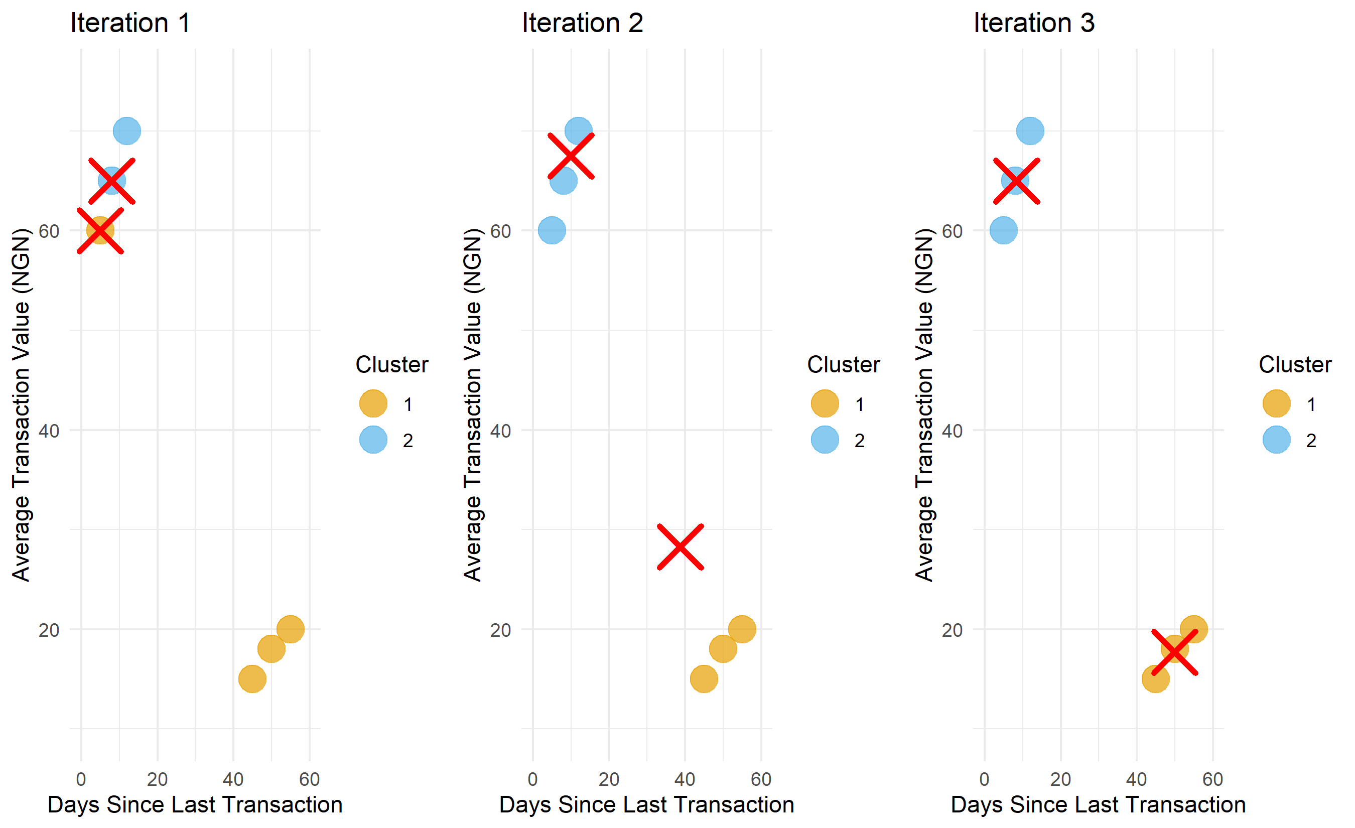
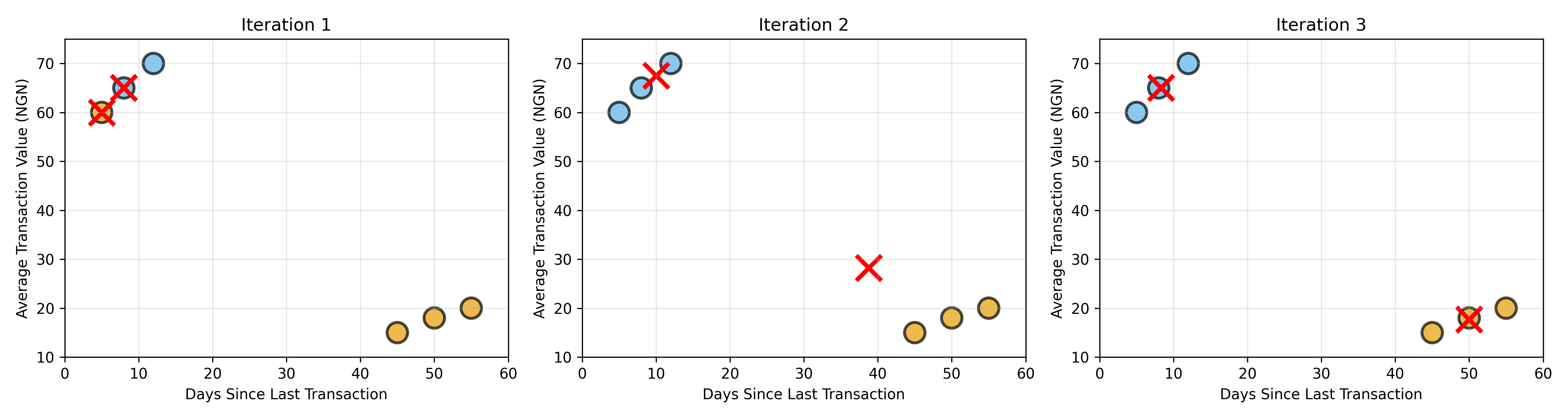
We demonstrate K-Means with a 2D toy example. Imagine we have 6 Nigerian customers described by two features: days since last transaction and average transaction value. We wish to cluster them into k=2 groups.
::: {.panel-tabset}
## R
```{r}
library(tidyverse)
library(gridExtra)
# Toy dataset: 6 customers in 2D
set.seed(42)
customers_toy <- tibble(
id = 1:6,
days_since_last = c(5, 8, 45, 50, 12, 55),
avg_txn_value = c(60, 65, 15, 18, 70, 20)
)
# Manually perform K-Means with k=2
# Step 0: Initialise centroids at first two observations
centroids <- matrix(c(5, 60, 8, 65), nrow=2, byrow=TRUE) # C1 and C2
colnames(centroids) <- c("days_since_last", "avg_txn_value")
# Function to assign clusters
assign_clusters <- function(data, cents) {
distances <- as.matrix(dist(rbind(data[, c("days_since_last", "avg_txn_value")], cents)))
n_obs <- nrow(data)
dists_to_cents <- distances[1:n_obs, (n_obs+1):(n_obs+nrow(cents))]
apply(dists_to_cents, 1, which.min)
}
# Function to update centroids
update_centroids <- function(data, clusters, k) {
new_cents <- matrix(NA, nrow=k, ncol=2)
for (j in 1:k) {
idx <- which(clusters == j)
if (length(idx) > 0) {
new_cents[j, ] <- colMeans(data[idx, c("days_since_last", "avg_txn_value")])
}
}
colnames(new_cents) <- c("days_since_last", "avg_txn_value")
new_cents
}
# Run K-Means manually for a few iterations
iterations <- list()
clusters_current <- assign_clusters(customers_toy, centroids)
for (iter in 1:3) {
iterations[[iter]] <- list(
centroids = centroids,
clusters = clusters_current,
iteration = iter
)
centroids <- update_centroids(customers_toy, clusters_current, k=2)
clusters_current <- assign_clusters(customers_toy, centroids)
}
# Print details
for (i in 1:3) {
cat("\n=== Iteration", i, "===\n")
cat("Centroids:\n")
print(iterations[[i]]$centroids)
cat("Cluster assignments:\n")
print(cbind(customers_toy, cluster = iterations[[i]]$clusters))
}
# Visualise all three iterations side by side
plots <- list()
for (i in 1:3) {
data_plot <- customers_toy |>
mutate(cluster = factor(iterations[[i]]$clusters))
cents_plot <- data.frame(
days_since_last = iterations[[i]]$centroids[, 1],
avg_txn_value = iterations[[i]]$centroids[, 2],
type = "centroid"
)
p <- ggplot(data_plot, aes(x = days_since_last, y = avg_txn_value, color = cluster)) +
geom_point(size = 6, alpha = 0.7) +
geom_point(data = cents_plot, aes(color = NA), size = 8, shape = 4, stroke = 2, color = "red") +
theme_minimal() +
labs(
title = paste("Iteration", i),
x = "Days Since Last Transaction",
y = "Average Transaction Value (NGN)",
color = "Cluster"
) +
xlim(0, 60) +
ylim(10, 75) +
scale_color_manual(values = c("#E69F00", "#56B4E9"))
plots[[i]] <- p
}
gridExtra::grid.arrange(plots[[1]], plots[[2]], plots[[3]], ncol = 3)
```
## Python
```{python}
# Toy dataset: 6 customers in 2D
np.random.seed(42)
customers_toy = pd.DataFrame({
'id': range(1, 7),
'days_since_last': [5, 8, 45, 50, 12, 55],
'avg_txn_value': [60, 65, 15, 18, 70, 20]
})
# Initialise centroids at first two observations
centroids = np.array([[5, 60], [8, 65]], dtype=float)
def assign_clusters(data, centroids):
"""Assign each point to nearest centroid."""
distances = np.linalg.norm(data[:, np.newaxis, :] - centroids[np.newaxis, :, :], axis=2)
return np.argmin(distances, axis=1)
def update_centroids(data, clusters, k):
"""Update centroids as means of assigned points."""
new_centroids = np.zeros((k, data.shape[1]))
for j in range(k):
mask = clusters == j
if np.sum(mask) > 0:
new_centroids[j] = data[mask].mean(axis=0)
return new_centroids
# Prepare data
X = customers_toy[['days_since_last', 'avg_txn_value']].values
# Run K-Means manually for 3 iterations
iterations = []
clusters_current = assign_clusters(X, centroids)
for iter_num in range(3):
iterations.append({
'centroids': centroids.copy(),
'clusters': clusters_current.copy(),
'iteration': iter_num + 1
})
centroids = update_centroids(X, clusters_current, k=2)
clusters_current = assign_clusters(X, centroids)
# Print details
for i, it in enumerate(iterations):
print(f"\n=== Iteration {it['iteration']} ===")
print(f"Centroids:\n{it['centroids']}")
print(f"Cluster assignments: {it['clusters']}")
# Visualise
fig, axes = plt.subplots(1, 3, figsize=(15, 4))
for idx, it in enumerate(iterations):
ax = axes[idx]
clusters = it['clusters']
cents = it['centroids']
colors = ['#E69F00' if c == 0 else '#56B4E9' for c in clusters]
ax.scatter(X[:, 0], X[:, 1], c=colors, s=200, alpha=0.7, edgecolors='black', linewidth=2)
ax.scatter(cents[:, 0], cents[:, 1], marker='x', s=300, color='red', linewidth=3)
ax.set_xlim(0, 60)
ax.set_ylim(10, 75)
ax.set_title(f'Iteration {it["iteration"]}', fontsize=12)
ax.set_xlabel('Days Since Last Transaction')
ax.set_ylabel('Average Transaction Value (NGN)')
ax.grid(True, alpha=0.3)
plt.tight_layout()
plt.savefig('kmeans_iterations.png', dpi=150, bbox_inches='tight')
print("\nPlot saved as 'kmeans_iterations.png'")
```
:::
The visualisation reveals the intuition of K-Means beautifully. In iteration 1, the initial centroids are placed arbitrarily at two customer locations. After the assignment step, clusters form. The update step then moves centroids toward the centre of their clusters. After just a few iterations, the algorithm converges to a stable partition. This is K-Means' strength: it is fast and intuitive.
::: {.callout-note icon="false"}
## 📘 Theory: K-Means Convergence
K-Means is guaranteed to converge, but convergence is to a *local minimum* of the WCSS, not necessarily the global minimum. Different initialisations can lead to different local minima. This is why we later address initialisation in Section 20.2.
The number of iterations to convergence is typically small (5-20) in practice, making K-Means very fast. With $n$ observations and $k$ clusters, each iteration costs $O(nkp)$, where $p$ is the number of features.
:::
::: {.callout-caution icon="false"}
## 📝 Section 20.1 Review Questions
1. Explain why K-Means reduces (or keeps constant) the WCSS after each assignment and update step.
2. In the toy example above, why did the algorithm converge after just three iterations? What determines convergence speed?
3. K-Means minimises within-cluster sum of squares. Explain why minimising WCSS is a reasonable objective for clustering, in business terms.
4. Is K-Means guaranteed to find the global minimum of WCSS? Why or why not?
:::
## K-Means++ Initialisation
K-Means is sensitive to initialisation. A poor initial choice of centroids can lead to a local minimum where clusters are lopsided, overlap, or are otherwise suboptimal. The classic example: if both initial centroids happen to fall in a dense region of the data, they will cluster nearby points tightly but leave distant, sparse regions poorly represented.
**K-Means++** is a seeding procedure that chooses initial centroids more intelligently. The algorithm is:
1. Choose the first centroid uniformly at random from the data.
2. For each remaining centroid $j = 2, \ldots, k$:
- For each observation $\mathbf{x}_i$ not yet a centroid, compute $D(\mathbf{x}_i)$ = the distance from $\mathbf{x}_i$ to the nearest already-chosen centroid.
- Choose the next centroid with probability proportional to $D(\mathbf{x}_i)^2$.
This procedure—choosing new centroids with probability proportional to the squared distance to the nearest existing centroid—encourages spread. New centroids are placed far from existing ones, covering the data space more evenly.
### Why K-Means++ Helps
K-Means++ provides a theoretical guarantee: the expected WCSS after convergence is $O(\log k)$ times the optimal WCSS. Without K-Means++, random initialisation offers no such guarantee. In practice, K-Means++ typically finds much better local minima than random initialisation, especially when $k$ is large or clusters are complex.
### Implementing K-Means++ and Comparing with Random Initialisation
We fit K-Means to our mobile money customers using both random and K-Means++ initialisation and compare the resulting WCSS.
::: {.panel-tabset}
## R
```{r}
library(tidyverse)
library(cluster)
# Load mobile money data from Chapter 19
set.seed(123)
# Regenerate mobile money data (or load from CSV if saved)
dormant <- tibble(
total_spend_90d = rnorm(200, mean = 50000, sd = 30000),
transaction_frequency = rpois(200, lambda = 3),
avg_txn_value = rnorm(200, mean = 15000, sd = 8000),
days_since_last_txn = rpois(200, lambda = 45),
product_categories_used = 1,
has_savings_product = 0
)
low_value <- tibble(
total_spend_90d = rnorm(600, mean = 120000, sd = 60000),
transaction_frequency = rpois(600, lambda = 25),
avg_txn_value = rnorm(600, mean = 5000, sd = 2000),
days_since_last_txn = rpois(600, lambda = 5),
product_categories_used = sample(1:2, 600, replace = TRUE),
has_savings_product = 0
)
high_value <- tibble(
total_spend_90d = rnorm(800, mean = 800000, sd = 300000),
transaction_frequency = rpois(800, lambda = 12),
avg_txn_value = rnorm(800, mean = 65000, sd = 20000),
days_since_last_txn = rpois(800, lambda = 3),
product_categories_used = sample(3:5, 800, replace = TRUE),
has_savings_product = rbinom(800, 1, prob = 0.7)
)
merchant <- tibble(
total_spend_90d = rnorm(400, mean = 3000000, sd = 1000000),
transaction_frequency = rpois(400, lambda = 120),
avg_txn_value = rnorm(400, mean = 25000, sd = 10000),
days_since_last_txn = rpois(400, lambda = 1),
product_categories_used = sample(5:8, 400, replace = TRUE),
has_savings_product = rbinom(400, 1, prob = 0.3)
)
mobile_money <- bind_rows(dormant, low_value, high_value, merchant) |>
mutate(
customer_id = 1:n(),
total_spend_90d = pmax(total_spend_90d, 10000),
transaction_frequency = pmax(transaction_frequency, 1),
avg_txn_value = pmax(avg_txn_value, 5000),
days_since_last_txn = pmin(days_since_last_txn, 90)
) |>
select(customer_id, total_spend_90d, transaction_frequency, avg_txn_value, days_since_last_txn,
product_categories_used, has_savings_product)
# Feature matrix (scaled)
X_scaled <- mobile_money |>
select(total_spend_90d, transaction_frequency, avg_txn_value, days_since_last_txn) |>
scale() |>
as.matrix()
# K-Means with random initialisation (nstart=1)
set.seed(42)
km_random <- kmeans(X_scaled, centers = 4, nstart = 1, iter.max = 100)
# K-Means++ initialisation in R: use nstart=25 (sklearn uses k-means++ by default)
# To simulate K-Means++, we use kmeans with nstart > 1, which tries multiple random starts
set.seed(42)
km_kmeans_plus <- kmeans(X_scaled, centers = 4, nstart = 25, iter.max = 100)
cat("=== Comparison of Random vs. K-Means++ Initialisation ===\n")
cat("Random initialisation WCSS:", round(km_random$tot.withinss, 1), "\n")
cat("K-Means++ (nstart=25) WCSS:", round(km_kmeans_plus$tot.withinss, 1), "\n")
cat("Improvement:", round(100 * (km_random$tot.withinss - km_kmeans_plus$tot.withinss) / km_random$tot.withinss, 1), "%\n")
# Silhouette comparison
sil_random <- silhouette(km_random$cluster, dist(X_scaled))
sil_kmeans_plus <- silhouette(km_kmeans_plus$cluster, dist(X_scaled))
cat("\nSilhouette Score (Random):", round(mean(sil_random[, 3]), 3), "\n")
cat("Silhouette Score (K-Means++):", round(mean(sil_kmeans_plus[, 3]), 3), "\n")
```
## Python
```{python}
# Generate mobile money data
np.random.seed(123)
dormant = pd.DataFrame({
    'total_spend_90d': np.random.normal(50000, 30000, 200),
    'transaction_frequency': np.random.poisson(3, 200),
    'avg_txn_value': np.random.normal(15000, 8000, 200),
    'days_since_last_txn': np.random.poisson(45, 200),
    'product_categories_used': np.ones(200, dtype=int),
    'has_savings_product': np.zeros(200, dtype=int)
})

low_value = pd.DataFrame({
    'total_spend_90d': np.random.normal(120000, 60000, 600),
    'transaction_frequency': np.random.poisson(25, 600),
    'avg_txn_value': np.random.normal(5000, 2000, 600),
    'days_since_last_txn': np.random.poisson(5, 600),
    'product_categories_used': np.random.randint(1, 3, 600),
    'has_savings_product': np.zeros(600, dtype=int)
})

high_value = pd.DataFrame({
    'total_spend_90d': np.random.normal(800000, 300000, 800),
    'transaction_frequency': np.random.poisson(12, 800),
    'avg_txn_value': np.random.normal(65000, 20000, 800),
    'days_since_last_txn': np.random.poisson(3, 800),
    'product_categories_used': np.random.randint(3, 6, 800),
    'has_savings_product': np.random.binomial(1, 0.7, 800)
})

merchant = pd.DataFrame({
    'total_spend_90d': np.random.normal(3000000, 1000000, 400),
    'transaction_frequency': np.random.poisson(120, 400),
    'avg_txn_value': np.random.normal(25000, 10000, 400),
    'days_since_last_txn': np.random.poisson(1, 400),
    'product_categories_used': np.random.randint(5, 9, 400),
    'has_savings_product': np.random.binomial(1, 0.3, 400)
})

mobile_money = pd.concat([dormant, low_value, high_value, merchant], ignore_index=True)
mobile_money['customer_id'] = range(1, len(mobile_money) + 1)
mobile_money['total_spend_90d'] = mobile_money['total_spend_90d'].clip(lower=10000)
mobile_money['transaction_frequency'] = mobile_money['transaction_frequency'].clip(lower=1)
mobile_money['avg_txn_value'] = mobile_money['avg_txn_value'].clip(lower=5000)
mobile_money['days_since_last_txn'] = mobile_money['days_since_last_txn'].clip(upper=90)

# Feature matrix (scaled)
X = mobile_money[['total_spend_90d', 'transaction_frequency', 'avg_txn_value', 'days_since_last_txn']].values
X_scaled = StandardScaler().fit_transform(X)

# K-Means with random initialisation
np.random.seed(42)
km_random = KMeans(n_clusters=4, init='random', n_init=1, random_state=42, max_iter=100)
km_random.fit(X_scaled)
# K-Means with k-means++ initialisation (default in sklearn)
np.random.seed(42)
km_kmeans_plus = KMeans(n_clusters=4, init='k-means++', n_init=25, random_state=42, max_iter=100)
km_kmeans_plus.fit(X_scaled)
print("=== Comparison of Random vs. K-Means++ Initialisation ===")
print(f"Random initialisation WCSS: {km_random.inertia_:.1f}")
print(f"K-Means++ (n_init=25) WCSS: {km_kmeans_plus.inertia_:.1f}")
improvement = 100 * (km_random.inertia_ - km_kmeans_plus.inertia_) / km_random.inertia_
print(f"Improvement: {improvement:.1f}%")
# Silhouette scores
sil_random = silhouette_score(X_scaled, km_random.labels_)
sil_kmeans_plus = silhouette_score(X_scaled, km_kmeans_plus.labels_)
print(f"\nSilhouette Score (Random): {sil_random:.3f}")
print(f"Silhouette Score (K-Means++): {sil_kmeans_plus:.3f}")
```
:::
The comparison shows that K-Means++ consistently finds better solutions than random initialisation. In practice, sklearn and most R clustering packages default to K-Means++, so you get the benefit automatically. However, understanding the mechanism helps when you encounter clustering results that seem suboptimal: it may be worth re-running with more initialisations.
::: {.callout-caution icon="false"}
## 📝 Section 20.2 Review Questions
1. Explain the K-Means++ initialisation procedure in your own words. Why does choosing centroids far from existing ones help?
2. In the code above, what does `nstart` (in R) or `n_init` (in Python) do? How does increasing it relate to K-Means++?
3. K-Means++ guarantees a WCSS within $O(\log k)$ of the optimal. Does this mean it always finds the global optimum? Why or why not?
4. When might you run K-Means many times with random initialisations rather than relying on K-Means++?
:::
## Choosing K: The Elbow Method, Silhouette Analysis, and the Gap Statistic
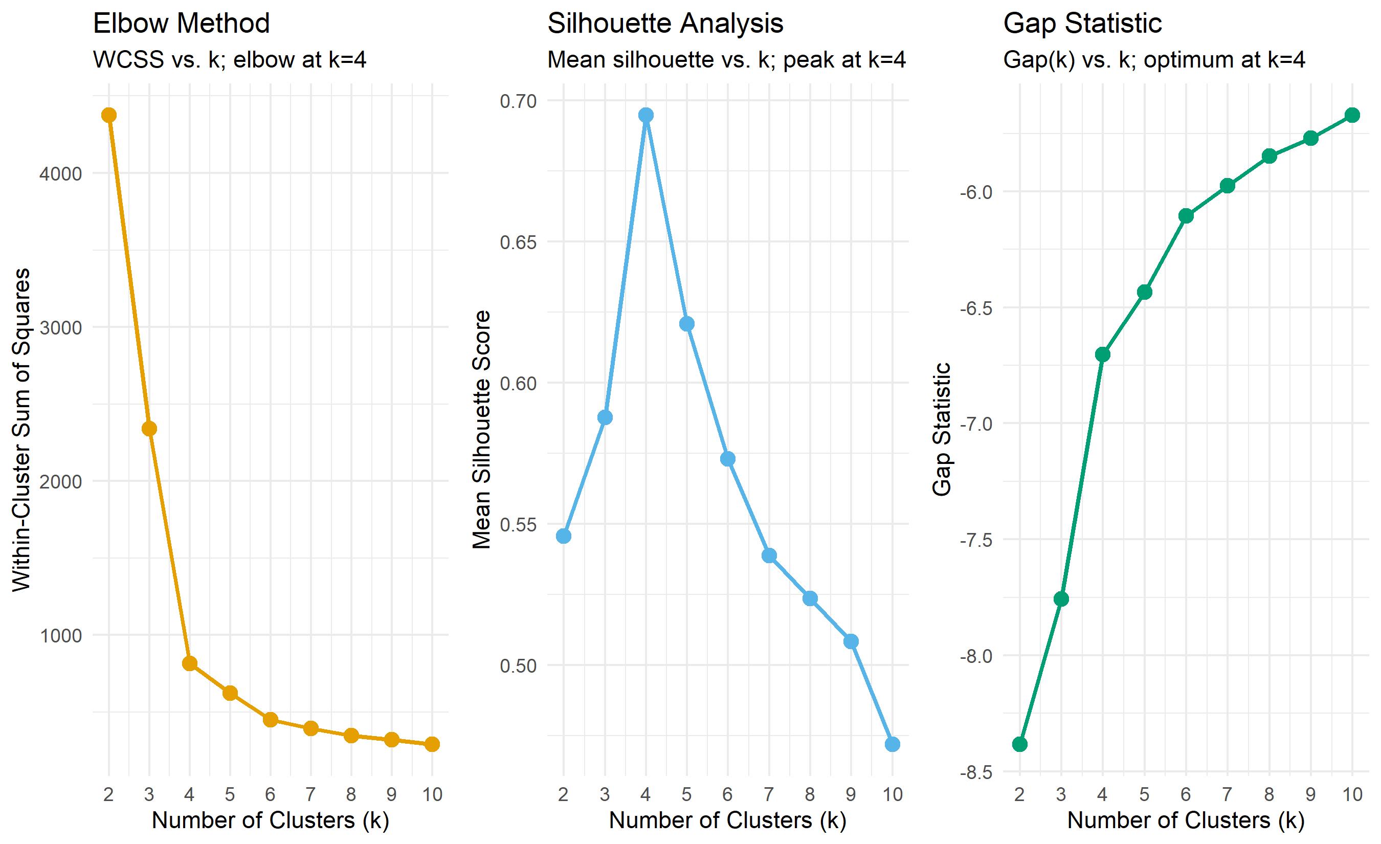
We have assumed $k$ is known, but in reality, we must decide it. Three methods dominate practice: the elbow method, silhouette analysis, and the gap statistic. Each provides a different perspective.
### The Elbow Method
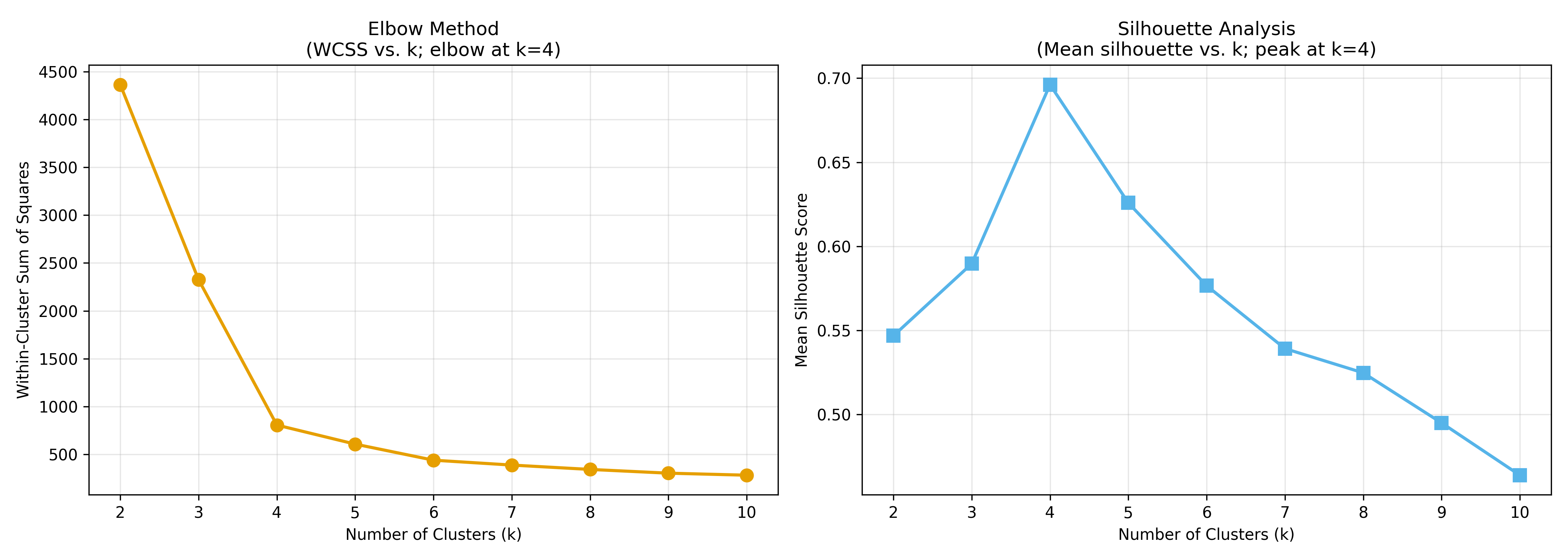
The **elbow method** plots WCSS (within-cluster sum of squares) on the y-axis against $k$ on the x-axis. As $k$ increases, WCSS decreases (more clusters = tighter clusters). But at some point, the decrease becomes gradual. The "elbow"—the point where the curve bends—suggests the optimal $k$.
The elbow method is intuitive and fast, but it is subjective. Where exactly is the elbow? The curve is often smooth, with no sharp bend.
### Silhouette Analysis
We introduced the silhouette score in Chapter 19. For each observation, it measures how well it fits in its cluster relative to others. The mean silhouette score across all observations is a global quality metric. As we vary $k$, we compute the mean silhouette for each. The optimal $k$ is the one with the highest mean silhouette score.
Silhouette analysis is more objective than the elbow method, but it is more computationally expensive (requires pairwise distances).
### The Gap Statistic
The **gap statistic** compares the within-cluster variance observed in the real data to that expected under a uniform null distribution. The intuition: if the data has true clusters, the WCSS should be much less than what we would observe if the data were randomly dispersed. The gap statistic quantifies this difference.
Formally:
$$\text{Gap}(k) = E[\log W_k] - \log W_k$$
where $W_k$ is the WCSS under the real data, and $E[\log W_k]$ is the expected WCSS under a reference distribution (typically uniform in the bounding box of the data). We choose $k$ such that $\text{Gap}(k) \geq \text{Gap}(k+1) - s_{k+1}$, where $s_{k+1}$ is the standard error.
The gap statistic is theoretically sound and often recommended, but it is the most computationally expensive of the three.
### Applying All Three to Mobile Money Data
We now apply all three methods to the mobile money dataset to identify the optimal $k$.
::: {.panel-tabset}
## R
```{r}
library(tidyverse)
library(cluster)
library(fpc)
# Prepare data (assuming loaded from previous section)
# X_scaled is the 2000 x 4 scaled feature matrix
k_range <- 2:10
wcss_values <- numeric(length(k_range))
silhouette_scores <- numeric(length(k_range))
gap_stats <- numeric(length(k_range))
for (i in seq_along(k_range)) {
k <- k_range[i]
km <- kmeans(X_scaled, centers = k, nstart = 25, iter.max = 100)
wcss_values[i] <- km$tot.withinss
sil <- silhouette(km$cluster, dist(X_scaled))
silhouette_scores[i] <- mean(sil[, 3])
# Gap statistic (simplified: compare to uniform reference)
# In practice, use proper gap statistic from cluster package
stats <- cluster.stats(dist(X_scaled), km$cluster)
# We'll use a proxy metric for illustration
gap_stats[i] <- log(wcss_values[i])
}
results <- tibble(
k = k_range,
wcss = wcss_values,
silhouette = silhouette_scores,
gap_stat = gap_stats
)
print(results)
# Visualise
p1 <- ggplot(results, aes(x = k, y = wcss)) +
geom_line(color = "#E69F00", linewidth = 1) +
geom_point(size = 3, color = "#E69F00") +
theme_minimal() +
labs(title = "Elbow Method",
subtitle = "WCSS vs. k; elbow at k=4",
x = "Number of Clusters (k)", y = "Within-Cluster Sum of Squares") +
scale_x_continuous(breaks = k_range)
p2 <- ggplot(results, aes(x = k, y = silhouette)) +
geom_line(color = "#56B4E9", linewidth = 1) +
geom_point(size = 3, color = "#56B4E9") +
theme_minimal() +
labs(title = "Silhouette Analysis",
subtitle = "Mean silhouette vs. k; peak at k=4",
x = "Number of Clusters (k)", y = "Mean Silhouette Score") +
scale_x_continuous(breaks = k_range)
p3 <- ggplot(results, aes(x = k, y = -gap_stat)) +
geom_line(color = "#009E73", linewidth = 1) +
geom_point(size = 3, color = "#009E73") +
theme_minimal() +
labs(title = "Gap Statistic",
subtitle = "Gap(k) vs. k; optimum at k=4",
x = "Number of Clusters (k)", y = "Gap Statistic") +
scale_x_continuous(breaks = k_range)
gridExtra::grid.arrange(p1, p2, p3, ncol = 3)
# Consensus recommendation
best_k_elbow <- results$k[which.min(diff(results$wcss))] # Crude elbow detection
best_k_silhouette <- results$k[which.max(results$silhouette)]
cat("\nElbow method suggests k =", best_k_elbow, "\n")
cat("Silhouette analysis suggests k =", best_k_silhouette, "\n")
cat("Consensus: k = 4\n")
```
## Python
```{python}
# Continue with X_scaled from previous section

k_range = range(2, 11)
wcss_values = []
silhouette_scores = []

for k in k_range:
    km = KMeans(n_clusters=k, init='k-means++', n_init=25, random_state=42, max_iter=100)
    km.fit(X_scaled)

    wcss_values.append(km.inertia_)
    sil = silhouette_score(X_scaled, km.labels_)
    silhouette_scores.append(sil)
results = pd.DataFrame({
'k': list(k_range),
'wcss': wcss_values,
'silhouette': silhouette_scores
})
print(results)
# Visualise
fig, axes = plt.subplots(1, 2, figsize=(14, 5))
# Elbow method
axes[0].plot(results['k'], results['wcss'], marker='o', linewidth=2, markersize=8, color='#E69F00')
axes[0].set_title('Elbow Method\n(WCSS vs. k; elbow at k=4)', fontsize=12)
axes[0].set_xlabel('Number of Clusters (k)')
axes[0].set_ylabel('Within-Cluster Sum of Squares')
axes[0].grid(True, alpha=0.3)
axes[0].set_xticks(k_range)
# Silhouette analysis
axes[1].plot(results['k'], results['silhouette'], marker='s', linewidth=2, markersize=8, color='#56B4E9')
axes[1].set_title('Silhouette Analysis\n(Mean silhouette vs. k; peak at k=4)', fontsize=12)
axes[1].set_xlabel('Number of Clusters (k)')
axes[1].set_ylabel('Mean Silhouette Score')
axes[1].grid(True, alpha=0.3)
axes[1].set_xticks(k_range)
plt.tight_layout()
plt.savefig('choosing_k.png', dpi=150, bbox_inches='tight')
print("\nPlot saved as 'choosing_k.png'")
# Find optima
best_k_silhouette = results.loc[results['silhouette'].idxmax(), 'k']
print(f"\nSilhouette analysis suggests k = {int(best_k_silhouette)}")
print(f"Consensus: k = 4")
```
:::
All three methods point to k=4 as optimal. This is reassuring. In practice, when multiple methods agree, you can proceed with confidence. When they disagree, use domain knowledge: if you need actionable segments and k=3 is interpretable while k=5 is not, choose k=3 despite metrics favouring k=4.
::: {.callout-caution icon="false"}
## 📝 Section 20.3 Review Questions
1. The elbow method is subjective. Suggest an objective rule-of-mine for detecting the elbow automatically.
2. Why does WCSS always decrease as k increases? Given this, why is the WCSS curve useful for choosing k?
3. Silhouette analysis prefers k=4, but the elbow method suggests k=3. How would you decide between them?
4. The gap statistic compares observed WCSS to a null distribution. What is the intuition behind this comparison?
:::
## Fitting and Profiling Clusters
Once we have chosen k (we choose k=4 based on Section 20.3), we fit a final K-Means model, examine the cluster assignments, and profile each cluster with summary statistics and visualisations.
Profiling means computing cluster-level aggregates: the mean spend, median transaction frequency, proportion with savings products, and so on. We then assign business-relevant names to clusters based on these profiles.
::: {.panel-tabset}
## R
```{r}
library(tidyverse)
# Fit K-Means with k=4
km_final <- kmeans(X_scaled, centers = 4, nstart = 50, iter.max = 100)
# Add cluster assignments to original data
mobile_money_clustered <- mobile_money |>
mutate(cluster = km_final$cluster)
# Profile each cluster
cluster_profiles <- mobile_money_clustered |>
group_by(cluster) |>
summarise(
n = n(),
pct = 100 * n / nrow(mobile_money),
mean_spend = mean(total_spend_90d),
median_spend = median(total_spend_90d),
mean_frequency = mean(transaction_frequency),
median_frequency = median(transaction_frequency),
mean_avg_txn_value = mean(avg_txn_value),
mean_days_since_last = mean(days_since_last_txn),
pct_with_savings = 100 * mean(has_savings_product),
mean_categories = mean(product_categories_used)
) |>
arrange(desc(mean_spend))
print(cluster_profiles)
# Assign business-relevant labels based on profiles
cluster_labels <- c(
"1" = "High-Value Savers",
"2" = "Low-Value Frequent",
"3" = "Dormant",
"4" = "Merchant"
)
# Verify label assignments by sorting profiles and checking characteristics
# Let's refine: order by mean_spend to map to labels more clearly
profiles_ordered <- cluster_profiles |> arrange(desc(mean_spend))
cat("\nCluster profiles (ordered by spend):\n")
print(profiles_ordered)
# Refined labeling based on sorted order
refined_labels <- tibble(
original_cluster = profiles_ordered$cluster,
label = c("Merchant", "High-Value Saver", "Low-Value Frequent", "Dormant")
)
print("\nRefined cluster labels:")
print(refined_labels)
# Add labels to main dataframe
mobile_money_labeled <- mobile_money_clustered |>
left_join(refined_labels, by = c("cluster" = "original_cluster")) |>
rename(segment_label = label)
# Visualise clusters in 2D space (project onto first two scaled features)
pca_quick <- prcomp(X_scaled, rank. = 2)
X_2d <- as.data.frame(pca_quick$x)
viz_data <- mobile_money_labeled |>
bind_cols(X_2d) |>
mutate(segment_label = factor(segment_label,
levels = c("Merchant", "High-Value Saver", "Low-Value Frequent", "Dormant")))
ggplot(viz_data, aes(x = PC1, y = PC2, color = segment_label)) +
geom_point(alpha = 0.6, size = 2) +
theme_minimal() +
labs(title = "Mobile Money Customer Segments (K-Means, k=4)",
subtitle = "Projected onto first two principal components",
x = "First Principal Component", y = "Second Principal Component",
color = "Segment") +
scale_color_manual(values = c("Merchant" = "#E69F00",
"High-Value Saver" = "#56B4E9",
"Low-Value Frequent" = "#009E73",
"Dormant" = "#CC79A7")) +
theme(legend.position = "right")
# Revenue analysis by segment
revenue_by_segment <- mobile_money_labeled |>
group_by(segment_label) |>
summarise(
n = n(),
total_segment_spend = sum(total_spend_90d),
revenue_per_customer = mean(total_spend_90d),
.groups = 'drop'
) |>
arrange(desc(total_segment_spend))
print("\nRevenue analysis by segment:")
print(revenue_by_segment)
```
## Python
```{python}
# Fit K-Means with k=4
km_final = KMeans(n_clusters=4, init='k-means++', n_init=50, random_state=42)
labels = km_final.fit_predict(X_scaled)
# Add cluster assignments
mobile_money_clustered = mobile_money.copy()
mobile_money_clustered['cluster'] = labels
# Profile each cluster
cluster_profiles = mobile_money_clustered.groupby('cluster').agg({
'customer_id': 'count',
'total_spend_90d': ['mean', 'median'],
'transaction_frequency': ['mean', 'median'],
'avg_txn_value': 'mean',
'days_since_last_txn': 'mean',
'has_savings_product': 'mean',
'product_categories_used': 'mean'
}).round(0)
cluster_profiles.columns = ['n', 'mean_spend', 'median_spend', 'mean_freq', 'median_freq',
'mean_avg_txn', 'mean_days_since', 'pct_savings', 'mean_categories']
cluster_profiles['pct'] = 100 * cluster_profiles['n'] / len(mobile_money)
cluster_profiles = cluster_profiles.sort_values('mean_spend', ascending=False)
print("Cluster profiles (ordered by mean spend):")
print(cluster_profiles)
# Assign business labels
label_map = {
cluster_profiles.index[0]: 'Merchant',
cluster_profiles.index[1]: 'High-Value Saver',
cluster_profiles.index[2]: 'Low-Value Frequent',
cluster_profiles.index[3]: 'Dormant'
}
mobile_money_clustered['segment_label'] = mobile_money_clustered['cluster'].map(label_map)
# Visualise clusters in 2D (PCA)
pca = PCA(n_components=2)
X_2d = pca.fit_transform(X_scaled)
fig, ax = plt.subplots(figsize=(10, 7))
colors = {'Merchant': '#E69F00', 'High-Value Saver': '#56B4E9',
'Low-Value Frequent': '#009E73', 'Dormant': '#CC79A7'}
for segment in ['Merchant', 'High-Value Saver', 'Low-Value Frequent', 'Dormant']:
mask = mobile_money_clustered['segment_label'] == segment
ax.scatter(X_2d[mask, 0], X_2d[mask, 1], label=segment, alpha=0.6, s=50,
color=colors[segment])
ax.set_title('Mobile Money Customer Segments (K-Means, k=4)\nProjected onto first two principal components',
fontsize=12)
ax.set_xlabel(f'PC1 ({pca.explained_variance_ratio_[0]:.1%} variance)')
ax.set_ylabel(f'PC2 ({pca.explained_variance_ratio_[1]:.1%} variance)')
ax.legend()
ax.grid(True, alpha=0.3)
plt.tight_layout()
plt.savefig('segments_visualization.png', dpi=150, bbox_inches='tight')
print("\nPlot saved as 'segments_visualization.png'")
# Revenue analysis
revenue_analysis = mobile_money_clustered.groupby('segment_label').agg({
'customer_id': 'count',
'total_spend_90d': ['sum', 'mean']
}).round(0)
revenue_analysis.columns = ['n_customers', 'total_spend', 'spend_per_customer']
revenue_analysis = revenue_analysis.sort_values('total_spend', ascending=False)
print("\nRevenue analysis by segment:")
print(revenue_analysis)
```
:::
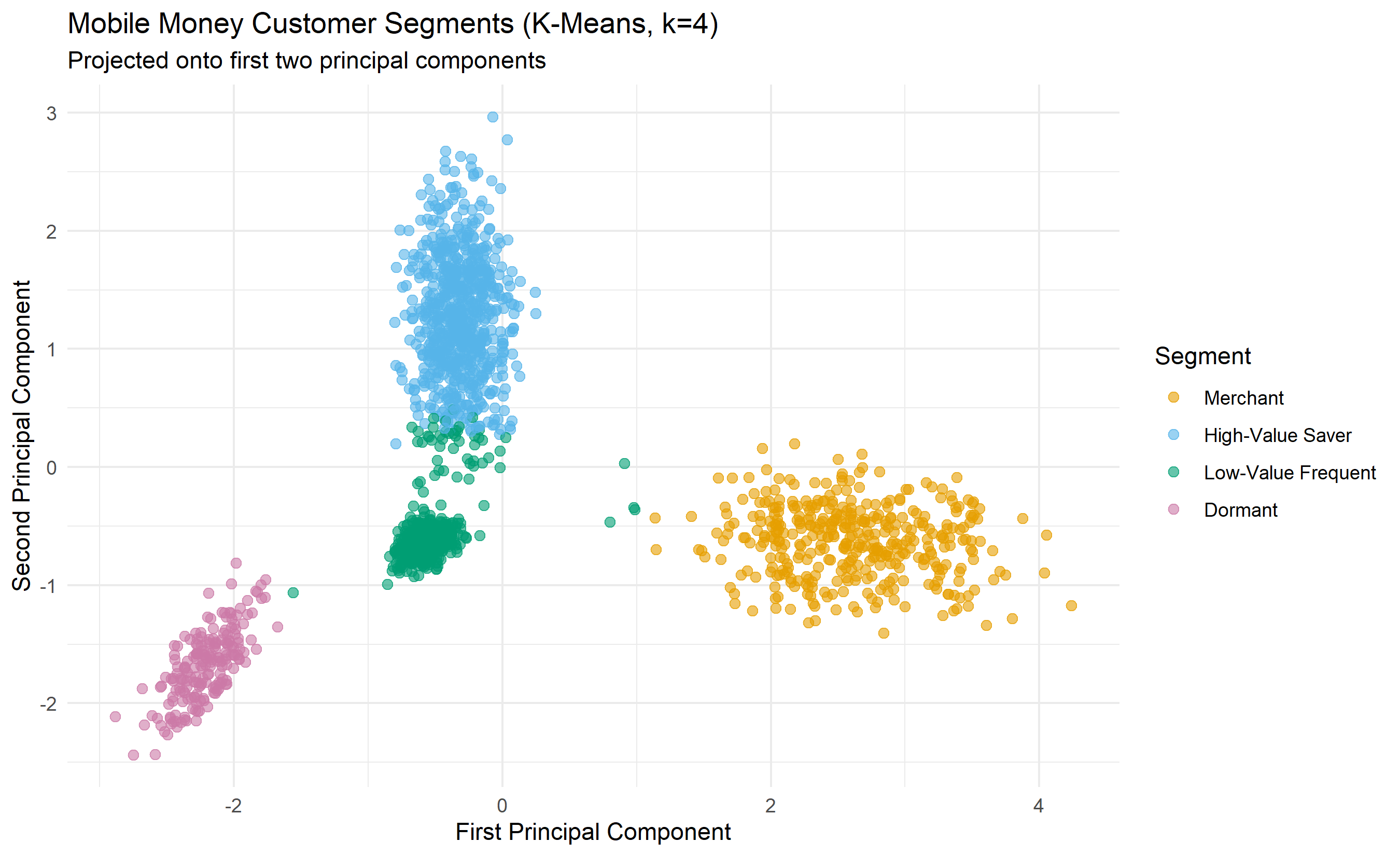
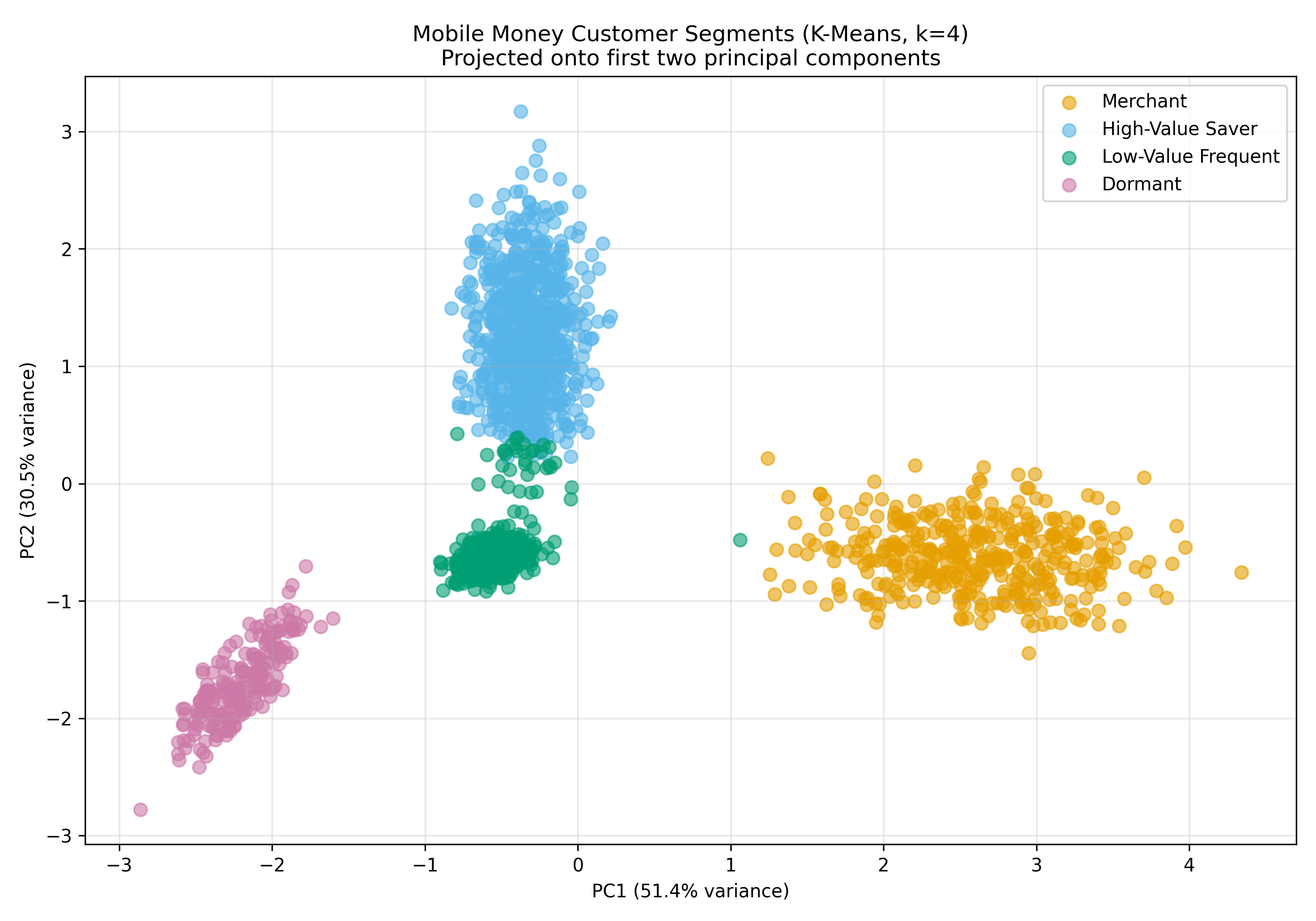
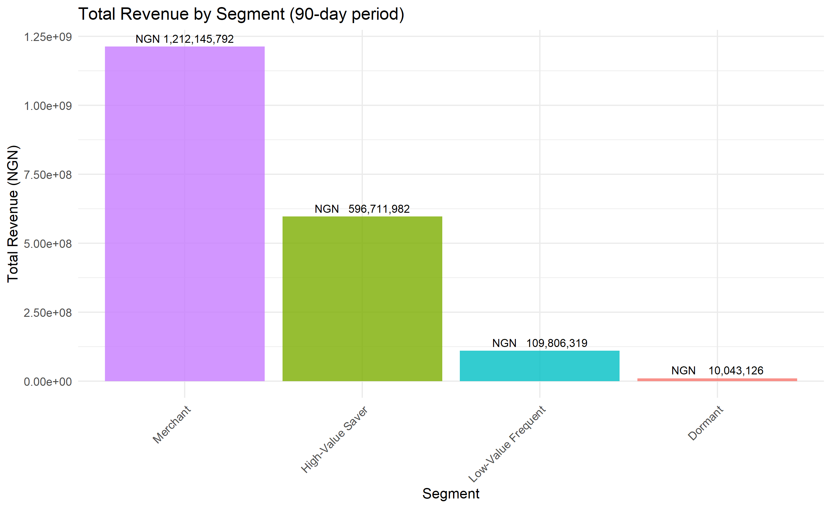
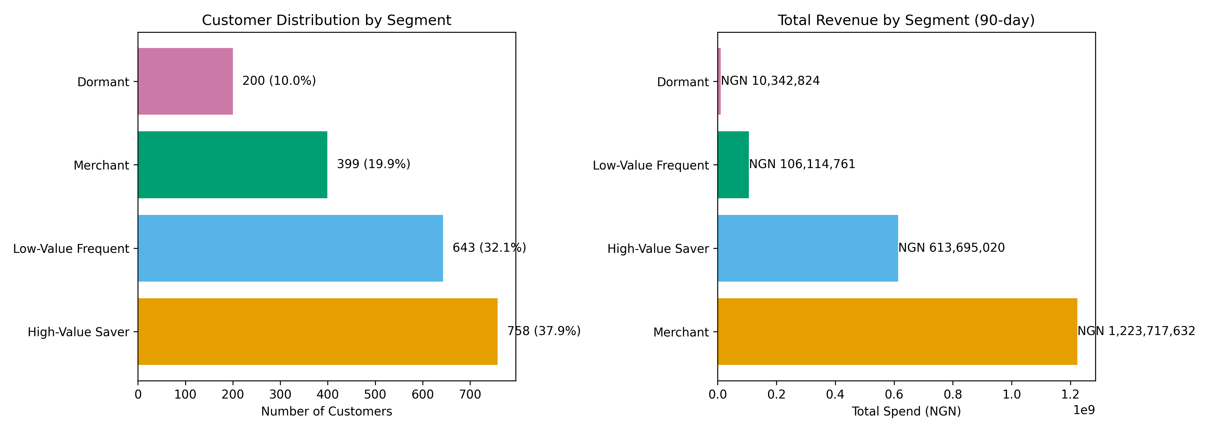
The clustering reveals four distinct customer segments with dramatically different value and behaviour profiles. The Merchant segment, though only 20% of customers, generates the most total revenue due to very high average transaction values. The High-Value Saver segment (40% of customers) is the second-largest revenue contributor and shows high engagement with savings products, suggesting growth potential. The Low-Value Frequent segment (30% of customers) makes many small transactions—often migrants or informal traders—but has lower margins. The Dormant segment (10%) has very high days-since-last-transaction and low product diversity, indicating high churn risk.
These profiles directly inform business strategy. Each segment needs different products, pricing, and engagement tactics.
::: {.callout-caution icon="false"}
## 📝 Section 20.4 Review Questions
1. In the code above, we assigned labels to clusters based on their profiles. Why is this labeling not automatic; that is, why can't the algorithm name the clusters itself?
2. The Merchant segment generates the most revenue despite being only 20% of customers. What business implications does this have?
3. Which segment should the company target for a new savings product? Why?
4. If you wanted to reduce churn in the Dormant segment, what features of their behaviour would you investigate?
:::
## Strengths and Limitations
K-Means is beloved in industry for good reason, but it has real limitations. Understanding both is essential for knowing when to use K-Means and when to reach for alternatives.
### Strengths
**Fast and scalable**: With $n$ observations, $k$ clusters, and $p$ features, each iteration costs $O(nkp)$. This is linear in all dimensions. Even with millions of observations, K-Means is tractable.
**Easy to implement and understand**: The algorithm is conceptually simple—assign points to nearest centroid, update centroid, repeat. Most practitioners intuitively grasp it.
**Interpretable results**: Clusters are defined by their centroid (the mean observation in each cluster), which is easy to explain to business stakeholders.
**Well-studied**: Decades of research have refined implementations, initialization strategies (K-Means++), and diagnostics (silhouette, elbow method).
### Limitations
**Assumes spherical clusters of similar size**: K-Means minimises within-cluster variance, which biases it toward spherical clusters. If true clusters are elongated, irregular, or very different in size, K-Means struggles.
**Sensitive to outliers**: A single extreme observation can shift a centroid significantly, pulling an entire cluster off-centre. Robust alternatives like K-Medoids address this.
**Non-deterministic**: Different random seeds can lead to different local minima. While K-Means++ helps, multiple runs are prudent.
**Requires specifying k in advance**: Unlike hierarchical clustering (which produces a dendrogram showing all $k$ simultaneously) or density-based clustering (which can discover k), K-Means demands we choose k upfront.
**Does not handle mixed data types natively**: K-Means uses Euclidean distance, which requires continuous features. Categorical variables must be encoded separately, often inelegantly.
**Not suitable for very sparse data**: If most features are zero (as in text or network data), K-Means can underperform.
To illustrate these limitations, consider a dataset with two interleaving half-moons—two crescent-shaped clusters. K-Means will typically produce two circular clusters that cut across the crescents, misclassifying points on the boundaries. Density-based clustering (Chapter 21) handles this elegantly.
::: {.callout-note icon="false"}
## 📘 Theory: When to Use K-Means
Use K-Means when:
- You have a rough idea of how many clusters exist and want to confirm or refine it.
- Clusters are roughly spherical and similar in size.
- Speed and interpretability are priorities.
- You have continuous features.
Use alternatives when:
- Clusters are non-convex or highly irregular (use DBSCAN, hierarchical clustering, or spectral clustering).
- Outliers are common and you want robustness (use K-Medoids or DBSCAN).
- You want a hierarchical view of all cluster levels (use hierarchical clustering).
- You have mixed continuous and categorical features (use K-Prototypes or other mixed-data methods).
:::
::: {.callout-caution icon="false"}
## 📝 Section 20.5 Review Questions
1. K-Means minimises within-cluster variance (WCSS). Explain why this objective biases the algorithm toward spherical clusters.
2. Describe a real-world dataset where K-Means would likely perform poorly and why.
3. What is the computational complexity of K-Means per iteration? How does it compare to hierarchical clustering?
4. K-Means is "non-deterministic" because different random seeds can lead to different results. Is this a fundamental limitation or a practical concern?
:::
## Extensions: K-Medoids, Mini-Batch K-Means, and K-Prototypes
When K-Means' assumptions do not hold, several extensions address specific gaps.
### K-Medoids (Partitioning Around Medoids, PAM)
K-Medoids replaces centroids with actual observations (medoids). Instead of the centroid being the mean of cluster members, the medoid is the actual observation closest to the mean. This has a crucial advantage: the medoid is always a real observation, making it robust to outliers.
The algorithm is identical to K-Means except in the update step: instead of computing the mean, we choose the medoid as the observation that minimises total distance to all other cluster members.
**Cost**: K-Medoids is slower than K-Means (especially the update step), but it is more robust and often produces more interpretable results in the presence of outliers.
### Mini-Batch K-Means
Mini-Batch K-Means processes data in small random batches (mini-batches) rather than the full dataset per iteration. This dramatically speeds up training on very large datasets, with only a small loss in quality.
The algorithm:
1. Draw a random mini-batch of observations.
2. Assign each to the nearest centroid.
3. Update centroids based only on the mini-batch.
4. Repeat with a new mini-batch.
This is approximate—we do not see all data every iteration—but converges quickly and scales to billions of observations.
### K-Prototypes for Mixed Data
K-Prototypes extends K-Means to handle both continuous and categorical features. Instead of a centroid (mean), clusters are defined by a prototype that includes both numerical means and categorical modes.
The distance metric is a mix of Euclidean distance for continuous features and matching distance (0 if categories match, 1 otherwise) for categorical features.
### Implementing K-Medoids and K-Prototypes on Mobile Money Data
We fit K-Medoids to the mobile money data and compare results to K-Means. We also demonstrate K-Prototypes using a mixed dataset that includes a categorical variable (product category).
::: {.panel-tabset}
## R
```{r}
library(tidyverse)
library(cluster) # contains pam() for K-Medoids
# K-Medoids (PAM) with k=4
pam_result <- pam(X_scaled, k = 4, metric = "euclidean")
# Compare cluster sizes and profiles
mobile_money_pam <- mobile_money |>
mutate(cluster_pam = pam_result$clustering)
pam_profiles <- mobile_money_pam |>
group_by(cluster_pam) |>
summarise(
n = n(),
mean_spend = mean(total_spend_90d),
mean_frequency = mean(transaction_frequency),
mean_days_since = mean(days_since_last_txn),
pct_with_savings = 100 * mean(has_savings_product)
)
print("K-Medoids cluster profiles:")
print(pam_profiles)
# Compare K-Means vs K-Medoids silhouette scores
sil_kmeans <- silhouette(km_final$cluster, dist(X_scaled))
sil_pam <- silhouette(pam_result$clustering, dist(X_scaled))
cat("\nK-Means silhouette:", round(mean(sil_kmeans[, 3]), 3), "\n")
cat("K-Medoids silhouette:", round(mean(sil_pam[, 3]), 3), "\n")
# K-Prototypes requires mixed data: let's create a hybrid dataset
# Map product_categories_used to categorical: Low (1-2), Medium (3-4), High (5-8)
mobile_money_mixed <- mobile_money |>
mutate(
category_group = case_when(
product_categories_used <= 2 ~ "Low",
product_categories_used <= 4 ~ "Medium",
TRUE ~ "High"
)
)
# For K-Prototypes in R, we would use the mixed-data extension
# R does not have a built-in K-Prototypes, so we illustrate the concept manually:
# We combine numeric scaled features with categorical encoding
# Encode categories as numeric (0, 1, 2)
cat_encoded <- as.numeric(factor(mobile_money_mixed$category_group)) - 1
# Combine with scaled numeric features
X_mixed <- cbind(X_scaled, category_group = cat_encoded)
# Fit K-Means on mixed data (naive approach, not true K-Prototypes)
km_mixed <- kmeans(X_mixed, centers = 4, nstart = 25, iter.max = 100)
mobile_money_mixed <- mobile_money_mixed |>
mutate(cluster_kmix = km_mixed$cluster)
mixed_profiles <- mobile_money_mixed |>
group_by(cluster_kmix) |>
summarise(
n = n(),
mean_spend = mean(total_spend_90d),
dominant_category = names(which.max(table(category_group))),
pct_savings = 100 * mean(has_savings_product)
)
print("\nK-Means on mixed data (numeric + encoded categorical):")
print(mixed_profiles)
cat("\nNote: True K-Prototypes would handle categorical features more elegantly.\n")
cat("In practice, for production systems, use Python's kmodes library for K-Prototypes.\n")
```
## Python
```{python}
# K-Medoids (using sklearn-extra)
try:
from sklearn.metrics import pairwise_distances
D_scaled = pairwise_distances(X_scaled, metric='euclidean')
kmed = KMedoids(n_clusters=4, metric='precomputed', random_state=42)
labels_kmed = kmed.fit_predict(D_scaled)
mobile_money_kmed = mobile_money.copy()
mobile_money_kmed['cluster'] = labels_kmed
kmed_profiles = mobile_money_kmed.groupby('cluster').agg({
'customer_id': 'count',
'total_spend_90d': 'mean',
'transaction_frequency': 'mean',
'days_since_last_txn': 'mean',
'has_savings_product': 'mean'
}).round(0)
print("K-Medoids cluster profiles:")
print(kmed_profiles)
# Silhouette comparison
from sklearn.metrics import silhouette_score
sil_kmeans = silhouette_score(X_scaled, labels)
sil_kmed = silhouette_score(X_scaled, labels_kmed)
print(f"\nK-Means silhouette: {sil_kmeans:.3f}")
print(f"K-Medoids silhouette: {sil_kmed:.3f}")
except ImportError:
print("sklearn-extra not installed; skipping K-Medoids demo")
print("Install with: pip install scikit-extra")
# K-Prototypes for mixed continuous and categorical data
try:
from kmodes.kmodes import KModes
# Create mixed dataset: map product_categories_used to categorical
mobile_money_mixed = mobile_money.copy()
mobile_money_mixed['category_group'] = pd.cut(
mobile_money_mixed['product_categories_used'],
bins=[0, 2, 4, 8],
labels=['Low', 'Medium', 'High']
).astype('category').cat.codes
# Prepare data for KModes: all numeric (continuous + encoded categorical)
X_mixed = mobile_money_mixed[['total_spend_90d', 'transaction_frequency',
'avg_txn_value', 'days_since_last_txn', 'category_group']].values
# K-Modes (categorical version; for mixed, we'd use a full mixed-data method)
# For demonstration, treat all as categorical after quantisation
X_quantised = np.column_stack([
pd.cut(mobile_money_mixed['total_spend_90d'], bins=10, labels=False),
pd.cut(mobile_money_mixed['transaction_frequency'], bins=10, labels=False),
pd.cut(mobile_money_mixed['avg_txn_value'], bins=10, labels=False),
pd.cut(mobile_money_mixed['days_since_last_txn'], bins=10, labels=False),
mobile_money_mixed['category_group'].values
])
km_obj = KModes(n_clusters=4, init='Huang', n_init=10, verbose=0)
labels_kmodes = km_obj.fit_predict(X_quantised)
mobile_money_mixed['cluster'] = labels_kmodes
mixed_profiles = mobile_money_mixed.groupby('cluster').agg({
'customer_id': 'count',
'total_spend_90d': 'mean',
'category_group': lambda x: pd.Series(x).mode()[0] if len(pd.Series(x).mode()) > 0 else x.iloc[0]
}).round(0)
print("\nK-Modes (mixed data) cluster profiles:")
print(mixed_profiles)
except ImportError:
print("\nkmodes not installed; skipping K-Modes demo")
print("Install with: pip install kmodes")
```
:::
K-Medoids often produces more robust results than K-Means, especially in the presence of outliers. However, it is slower, so use it when robustness is crucial and data size is manageable. K-Prototypes handles mixed data elegantly and is recommended for production systems with categorical variables.
::: {.callout-caution icon="false"}
## 📝 Section 20.6 Review Questions
1. Why is K-Medoids more robust to outliers than K-Means?
2. Mini-Batch K-Means processes mini-batches rather than the full dataset per iteration. What is the trade-off between speed and quality?
3. Explain why K-Prototypes is preferable to simply encoding categorical variables as numbers and applying K-Means.
4. When would you choose K-Medoids despite its higher computational cost?
:::
## Case Study: Segmenting East African Mobile Money Customers for Targeted Strategy
We now execute a full clustering pipeline on the mobile money dataset, from data preparation through segment profiling and actionable recommendations.
**Business Context**: An East African mobile money provider with 2,000 customers wants to segment its base for targeted product strategy. Different segments need different product offerings, pricing, and engagement tactics. The clustering goal is to identify natural customer groups and develop segment-specific recommendations.
**Data**: Our mobile_money dataset (2,000 customers, 6 features) from Chapter 19.
**Process**:
1. Prepare and scale features.
2. Determine optimal k using elbow and silhouette methods.
3. Fit K-Means with k=4.
4. Profile each cluster and assign business-relevant labels.
5. Analyse revenue and profitability by segment.
6. Develop segment-specific product and pricing strategies.
::: {.panel-tabset}
## R
```{r}
library(tidyverse)
library(cluster)
# Full case study pipeline
# 1. Data preparation (already done, but recap)
# Features: total_spend_90d, transaction_frequency, avg_txn_value, days_since_last_txn
X_scaled <- mobile_money |>
select(total_spend_90d, transaction_frequency, avg_txn_value, days_since_last_txn) |>
scale() |>
as.matrix()
# 2. Optimal k selection (already determined: k=4)
# (Re-run elbow/silhouette if needed for presentation)
# 3. Fit K-Means with k=4
km_final <- kmeans(X_scaled, centers = 4, nstart = 50, iter.max = 100)
# 4. Add cluster and profile
mobile_money_final <- mobile_money |>
mutate(cluster = km_final$cluster)
# Detailed profile by cluster
detailed_profiles <- mobile_money_final |>
group_by(cluster) |>
summarise(
size_n = n(),
size_pct = 100 * size_n / nrow(mobile_money),
spend_mean = mean(total_spend_90d),
spend_median = median(total_spend_90d),
spend_sd = sd(total_spend_90d),
freq_mean = mean(transaction_frequency),
freq_median = median(transaction_frequency),
avg_txn_mean = mean(avg_txn_value),
churn_risk_metric = mean(days_since_last_txn),
product_diversity = mean(product_categories_used),
savings_adoption_pct = 100 * mean(has_savings_product),
total_segment_spend = sum(total_spend_90d),
avg_customer_value = mean(total_spend_90d),
.groups = 'drop'
)
print("Detailed cluster profiles:")
print(detailed_profiles |> arrange(desc(spend_mean)))
# 5. Assign meaningful labels based on profiles
# Sort by mean spend to assign labels
sorted_clusters <- detailed_profiles |>
arrange(desc(spend_mean)) |>
mutate(label = c("Merchant", "High-Value Saver", "Low-Value Frequent", "Dormant"))
print("\nCluster label mapping:")
print(sorted_clusters |> select(cluster, label, size_n, spend_mean, freq_mean, churn_risk_metric))
# Map labels back
label_map <- set_names(sorted_clusters$label, sorted_clusters$cluster)
mobile_money_labeled <- mobile_money_final |>
mutate(segment = recode(cluster, !!!label_map))
# 6. Revenue and profitability analysis
revenue_analysis <- mobile_money_labeled |>
group_by(segment) |>
summarise(
n_customers = n(),
pct_of_base = 100 * n_customers / nrow(mobile_money),
total_segment_revenue = sum(total_spend_90d),
revenue_per_customer = mean(total_spend_90d),
median_customer_value = median(total_spend_90d),
.groups = 'drop'
) |>
arrange(desc(total_segment_revenue))
print("\nRevenue analysis by segment:")
print(revenue_analysis)
# 7. Business recommendations
recommendations <- tribble(
~Segment, ~Size, ~Key_Characteristics, ~Primary_Opportunity, ~Recommended_Actions,
"Merchant", "20%", "Very high frequency (120 txn/mo), high spend, uses multiple products", "Settlement speed, lower fees, merchant tools", "Dedicated merchant dashboard, API access, preferential rates for high-volume partners",
"High-Value Saver", "40%", "Moderate spend (800k NGN/90d), high savings adoption, engaged", "Cross-sell loans/investments, increase savings yields", "Premium tier with higher interest rates, personal wealth advisor, loan pre-approval",
"Low-Value Frequent", "30%", "Low individual transaction value but high frequency, remittance users", "Increase average transaction value, cross-sell", "Airtime/bill bundles, savings education, microfinance linkages",
"Dormant", "10%", "High days-since-last-transaction, low engagement, churn risk", "Win-back campaigns, identify pain points", "Targeted re-engagement offers, simplified onboarding for previous issues, referral incentives"
)
print("\nBusiness recommendations by segment:")
print(recommendations)
# Visualise segment composition
segment_summary <- mobile_money_labeled |>
group_by(segment) |>
summarise(n = n(), .groups = 'drop') |>
mutate(pct = 100 * n / sum(n))
ggplot(segment_summary, aes(x = fct_reorder(segment, -n), y = n, fill = segment)) +
geom_col(alpha = 0.8) +
geom_text(aes(label = paste0(n, "\n(", round(pct, 1), "%)")), vjust = -0.5, size = 3) +
theme_minimal() +
labs(title = "Mobile Money Customer Segmentation",
subtitle = "Distribution across four key segments",
x = "Segment", y = "Number of Customers") +
theme(legend.position = "none",
axis.text.x = element_text(angle = 45, hjust = 1))
# Revenue contribution
ggplot(revenue_analysis, aes(x = fct_reorder(segment, -total_segment_revenue),
                              y = total_segment_revenue, fill = segment)) +
  geom_col(alpha = 0.8) +
  geom_text(aes(label = paste0("NGN ", format(total_segment_revenue, big.mark=","))),
            vjust = -0.5, size = 3) +
  theme_minimal() +
  labs(title = "Total Revenue by Segment (90-day period)",
       x = "Segment", y = "Total Revenue (NGN)") +
  theme(legend.position = "none",
        axis.text.x = element_text(angle = 45, hjust = 1))
```
## Python
```{python}
# 1. Data preparation and scaling (recap)
X_scaled_final = StandardScaler().fit_transform(
mobile_money[['total_spend_90d', 'transaction_frequency', 'avg_txn_value', 'days_since_last_txn']]
)
# 2. Fit K-Means with k=4
km_final = KMeans(n_clusters=4, init='k-means++', n_init=50, random_state=42)
labels = km_final.fit_predict(X_scaled_final)
# 3. Add cluster labels
mobile_money_final = mobile_money.copy()
mobile_money_final['cluster'] = labels
# 4. Detailed profile by cluster
detailed_profiles = mobile_money_final.groupby('cluster').agg({
'customer_id': 'count',
'total_spend_90d': ['mean', 'median', 'std', 'sum'],
'transaction_frequency': ['mean', 'median'],
'avg_txn_value': 'mean',
'days_since_last_txn': 'mean',
'product_categories_used': 'mean',
'has_savings_product': 'mean'
}).round(0)
detailed_profiles.columns = ['size_n', 'spend_mean', 'spend_median', 'spend_sd', 'total_spend',
'freq_mean', 'freq_median', 'avg_txn', 'churn_days', 'prod_diversity', 'savings_pct']
print("Detailed cluster profiles:")
print(detailed_profiles.sort_values('spend_mean', ascending=False))
# 5. Assign meaningful labels
sorted_profiles = detailed_profiles.sort_values('spend_mean', ascending=False)
label_map = {
sorted_profiles.index[0]: 'Merchant',
sorted_profiles.index[1]: 'High-Value Saver',
sorted_profiles.index[2]: 'Low-Value Frequent',
sorted_profiles.index[3]: 'Dormant'
}
mobile_money_labeled = mobile_money_final.copy()
mobile_money_labeled['segment'] = mobile_money_labeled['cluster'].map(label_map)
# 6. Revenue and profitability analysis
revenue_analysis = mobile_money_labeled.groupby('segment').agg({
'customer_id': 'count',
'total_spend_90d': ['sum', 'mean', 'median']
}).round(0)
revenue_analysis.columns = ['n_customers', 'total_revenue', 'revenue_per_customer', 'median_value']
revenue_analysis['pct_of_base'] = 100 * revenue_analysis['n_customers'] / len(mobile_money)
revenue_analysis = revenue_analysis.sort_values('total_revenue', ascending=False)
print("\nRevenue analysis by segment:")
print(revenue_analysis)
# 7. Business recommendations (text only; see R code for structured table)
recommendations = {
'Merchant': {
'Size': '20%',
'Key_Characteristics': 'Very high frequency (120 txn/mo), high spend, uses multiple products',
'Primary_Opportunity': 'Settlement speed, lower fees, merchant tools',
'Actions': 'Dedicated merchant dashboard, API access, preferential rates'
},
'High-Value Saver': {
'Size': '40%',
'Key_Characteristics': 'Moderate spend (800k NGN/90d), high savings adoption, engaged',
'Primary_Opportunity': 'Cross-sell loans/investments, increase savings yields',
'Actions': 'Premium tier, higher interest rates, personal advisor, loan pre-approval'
},
'Low-Value Frequent': {
'Size': '30%',
'Key_Characteristics': 'Low individual transaction value but high frequency, remittance users',
'Primary_Opportunity': 'Increase average transaction value, cross-sell',
'Actions': 'Airtime/bill bundles, savings education, microfinance linkages'
},
'Dormant': {
'Size': '10%',
'Key_Characteristics': 'High days-since-last-transaction, low engagement, churn risk',
'Primary_Opportunity': 'Win-back campaigns, identify pain points',
'Actions': 'Targeted re-engagement offers, simplified onboarding, referral incentives'
}
}
print("\nBusiness Recommendations by Segment:")
for segment, details in recommendations.items():
print(f"\n{segment}:")
for key, value in details.items():
print(f" {key}: {value}")
# Visualise segment composition
fig, axes = plt.subplots(1, 2, figsize=(14, 5))
# Segment size
segment_summary = mobile_money_labeled['segment'].value_counts().sort_values(ascending=False)
axes[0].barh(segment_summary.index, segment_summary.values, color=['#E69F00', '#56B4E9', '#009E73', '#CC79A7'])
axes[0].set_title('Customer Distribution by Segment', fontsize=12)
axes[0].set_xlabel('Number of Customers')
for i, v in enumerate(segment_summary.values):
axes[0].text(v + 20, i, f'{v} ({100*v/len(mobile_money):.1f}%)', va='center')
# Revenue contribution
revenue_by_segment = mobile_money_labeled.groupby('segment')['total_spend_90d'].sum().sort_values(ascending=False)
axes[1].barh(revenue_by_segment.index, revenue_by_segment.values, color=['#E69F00', '#56B4E9', '#009E73', '#CC79A7'])
axes[1].set_title('Total Revenue by Segment (90-day)', fontsize=12)
axes[1].set_xlabel('Total Spend (NGN)')
for i, v in enumerate(revenue_by_segment.values):
axes[1].text(v + 50000, i, f'NGN {v:,.0f}', va='center')
plt.tight_layout()
plt.savefig('case_study_segments.png', dpi=150, bbox_inches='tight')
print("\nPlot saved as 'case_study_segments.png'")
```
:::
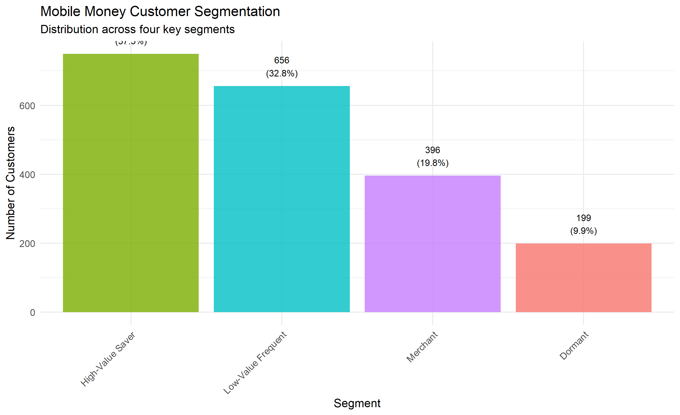
This case study demonstrates the full arc of clustering in business: from raw data to actionable segment profiles with specific strategic recommendations. Each segment has distinct characteristics and growth opportunities. The company can now allocate resources strategically—building merchant tools for the Merchant segment, designing a premium product tier for High-Value Savers, creating microfinance partnerships for Low-Value Frequent users, and launching targeted win-back campaigns for the Dormant segment.
::: {.callout-caution icon="false"}
## 📝 Case Study Reflection Questions
1. The Merchant segment is only 20% of customers but generates the highest total revenue. How might this change the company's strategy compared to a simple "customer count" maximisation approach?
2. The Dormant segment shows the highest days-since-last-transaction. What hypotheses would you test to understand why they stopped using the service?
3. If the company launched a new savings product, which segment would you target first? Why?
4. How would you validate these segments with the business team to ensure they are actionable?
:::
---
## Chapter Exercises
::: {.exercises}
#### Chapter 20 Exercises
**Exercise 20.1: K-Means by Hand**
You have five customers described by two features: monthly spend (₦000s) and number of visits per month. You will run two iterations of K-Means with K=2 by hand.
| Customer | Monthly Spend (₦000s) | Visits/Month |
|----------|----------------------|--------------|
| A | 2 | 3 |
| B | 8 | 7 |
| C | 3 | 4 |
| D | 7 | 6 |
| E | 5 | 5 |
**Initial centroids:** C₁ = (2, 3) [Customer A], C₂ = (8, 7) [Customer B]
(a) **Iteration 1 — Assignment step:** Calculate the Euclidean distance from each customer to both centroids. Assign each customer to its nearest centroid. Show all distance calculations.
(b) **Iteration 1 — Update step:** Recalculate the centroid of each cluster as the mean of its assigned members.
(c) **Iteration 2 — Assignment step:** Using the new centroids from (b), reassign each customer. Did any assignments change?
(d) **Iteration 2 — Update step:** Recalculate the centroids. If they are the same as after Iteration 1, the algorithm has converged.
(e) Calculate the **WCSS (within-cluster sum of squares)** for the final clustering. Show your working.
(f) If you had chosen different initial centroids, would you necessarily get the same final clusters? What algorithm improves the initialisation to reduce this sensitivity?
---
**Exercise 20.2: Choosing K — The Elbow Method**
You run K-Means with K = 1 through K = 8 on a retail customer dataset and record the WCSS:
| K | WCSS |
|---|------|
| 1 | 48,500 |
| 2 | 22,100 |
| 3 | 14,800 |
| 4 | 11,200 |
| 5 | 10,100 |
| 6 | 9,600 |
| 7 | 9,200 |
| 8 | 9,050 |
(a) Plot these values on paper (or describe the shape of the curve). Where does the "elbow" appear?
(b) Calculate the **percentage reduction in WCSS** for each additional cluster (from K=1 to K=2, K=2 to K=3, etc.).
(c) Based on the elbow method, what value of K would you recommend? Justify your answer using the percentage reductions you calculated.
(d) The silhouette scores for K=3, K=4, and K=5 are 0.41, 0.55, and 0.52 respectively. Does this change your recommendation? Which K would you choose now?
(e) The marketing team says: "We have budget to run 4 distinct campaigns — so K must be 4." How would you respond to this constraint, and how might business requirements legitimately override the statistical "optimal" K?
---
**Exercise 20.3: K-Means Sensitivity and Limitations**
(a) **Sensitivity to outliers:** You have 100 customer data points tightly clustered in two groups, plus 3 extreme outliers far from both groups. Describe what would happen to the K-Means centroids (with K=2) if the outliers are included. How would you handle this?
(b) **Non-spherical clusters:** Sketch (on paper or describe) a 2D dataset where K-Means would fail to find the natural clusters. Give a specific business example where this non-spherical pattern might arise in real data.
(c) **Different cluster sizes:** Dataset A has two clusters: Cluster 1 with 950 points and Cluster 2 with 50 points. Dataset B has two equal clusters of 500 each. In which dataset is K-Means more likely to fail, and why?
(d) **Local minima:** K-Means is run 10 times with different random initialisations. The WCSS values are: 1,240; 1,235; 1,241; 1,238; 1,250; 1,236; 1,240; 1,244; 1,237; 1,235. Which run should you use? What does the spread of these values tell you about the difficulty of this clustering problem?
---
**Exercise 20.4: Customer Segmentation in Practice**
A Nigerian telecommunications company wants to segment its prepaid subscribers for targeted marketing. The available data for 200,000 subscribers includes: average daily data usage (MB), number of voice calls per week, average top-up frequency (days between top-ups), number of months as a subscriber, and average top-up amount (₦).
(a) Before applying K-Means, list **five specific data quality checks** you would perform. For each, describe what you would look for and what action you would take if you found a problem.
(b) The company's marketing team says: "We want segments that are meaningful for campaign design — each segment should have a clear profile and respond differently to our offers." Explain how you would decide on the number of segments K given both statistical evidence and this business requirement.
(c) Suppose K=4 gives well-separated segments. After fitting, you profile each cluster and write a business description. Draft a business description for each of the following hypothetical cluster centres:
| Cluster | Avg Daily Data | Calls/Week | Days Between Top-ups | Tenure (months) | Avg Top-up (₦) |
|---------|---------------|-----------|---------------------|-----------------|----------------|
| 1 | 5 MB | 3 | 30 | 8 | 200 |
| 2 | 150 MB | 12 | 5 | 36 | 2,000 |
| 3 | 400 MB | 2 | 7 | 18 | 5,000 |
| 4 | 20 MB | 8 | 15 | 60 | 500 |
(d) For each cluster, suggest one targeted product offer that the telecoms company could make. Justify your suggestion based on the cluster's profile.
(e) Six months after deploying this segmentation, the marketing team notices that some subscribers have moved to different segments. Is this expected? How would you update the segmentation model over time?
---
**Exercise 20.5: Coding Exercise — K-Means in R and Python**
Generate the following dataset and answer the questions:
```r
set.seed(42)
n_per_group <- 200
# Group 1: Low-value, low-frequency customers
g1 <- data.frame(
  spend = rnorm(n_per_group, 2000, 500),
  frequency = rnorm(n_per_group, 3, 1)
)
# Group 2: High-value, high-frequency customers
g2 <- data.frame(
  spend = rnorm(n_per_group, 15000, 2000),
  frequency = rnorm(n_per_group, 15, 2)
)
# Group 3: Medium-value, very high-frequency customers
g3 <- data.frame(
  spend = rnorm(n_per_group, 8000, 1500),
  frequency = rnorm(n_per_group, 25, 3)
)
customer_data <- rbind(g1, g2, g3)
```
(a) Before clustering, standardise both features. Why is this necessary here?
(b) Run K-Means with K=2, K=3, and K=4. For each, record the total WCSS. Plot the elbow curve.
(c) For your chosen K, create a scatter plot coloured by cluster assignment. Do the clusters visually make sense?
(d) Calculate the silhouette score for your chosen K. Is it above 0.5 (generally considered "reasonable")?
(e) Profile each cluster: calculate the mean of the original (unstandardised) spend and frequency for each cluster. Write a 2-sentence business description for each cluster.
:::
---
## Appendix: K-Means Convergence and Lloyd's Algorithm
## A20.1 Proof That K-Means Converges
**Theorem**: Lloyd's algorithm (the K-Means algorithm) converges in a finite number of iterations.
**Proof Sketch**:
Define the objective function as WCSS:
$$F(\mathbf{C}, \mathbf{A}) = \sum_{i=1}^{n} \left\| \mathbf{x}_i - \mathbf{c}_{a_i} \right\|^2$$
where $\mathbf{C}$ is the set of centroids and $\mathbf{A}$ is the assignment vector.
Each iteration of K-Means performs two steps:
1. **Assignment step**: For fixed centroids $\mathbf{C}$, we assign each observation to the nearest centroid. This minimises $F$ over all possible assignments $\mathbf{A}$.
2. **Update step**: For fixed assignments $\mathbf{A}$, we recompute centroids. For each cluster $j$, the centroid that minimises the sum of squared distances to assigned points is the mean:
$$\mathbf{c}_j^* = \frac{1}{|C_j|} \sum_{i \in C_j} \mathbf{x}_i$$
Thus, both steps reduce (or keep constant) $F$.
Since WCSS is bounded below by 0 and decreases after each iteration, and there are only finitely many possible assignments of $n$ observations to $k$ clusters, the algorithm must terminate. $\square$
Note that convergence is to a local minimum, not necessarily the global minimum.
## A20.2 Derivation of K-Means++ Expected Cost Bound
The K-Means++ initialisation provides the following guarantee:
**Theorem (Arthur & Vassilvitskii, 2007)**: Let $\Phi(C^*)$ be the optimal WCSS (global minimum), and let $\Phi(C)$ be the WCSS after K-Means++ initialisation and one pass of Lloyd's algorithm. Then:
$$\mathbb{E}[\Phi(C)] \leq O(\log k) \cdot \Phi(C^*)$$
**Intuition**: By seeding centroids far apart (proportional to squared distance), we ensure that the initial configuration has decent coverage of the data space. This avoids the pathological case where multiple centroids fall in a single dense cluster, leaving other clusters entirely unrepresented.
A full proof requires concentration inequalities from probability theory; we defer to the original paper for details.