---
title: "Logistic Regression"
---
```{python}
#| label: python-setup-13-logistic-regression
#| include: false
import numpy as np
import pandas as pd
import matplotlib.pyplot as plt
import seaborn as sns
from sklearn.linear_model import LogisticRegression
import statsmodels.api as sm
from scipy.optimize import minimize
from sklearn.metrics import roc_auc_score
from sklearn.preprocessing import StandardScaler
from sklearn.linear_model import SGDClassifier
from sklearn.metrics import accuracy_score, precision_score, recall_score, f1_score, roc_auc_score
from sklearn.model_selection import train_test_split
```
::: {.callout-note icon="false"}
## 📋 Learning Objectives
By the end of this chapter, you will be able to:
- Understand why linear regression fails for classification and when logistic regression is needed
- Fit logistic regression models using maximum likelihood estimation
- Interpret logistic regression coefficients in terms of odds and odds ratios
- Construct and evaluate logistic regression models on real data
- Apply regularisation (L1 and L2) to logistic regression
- Build credit risk scorecards from logistic regression coefficients
- Evaluate model calibration and discrimination
- Use Weight of Evidence (WOE) and Information Value (IV) for feature selection
:::
## Why Not Linear Regression for Classification?
Linear regression predicts a **continuous value**. For classification, we need **bounded predictions** between 0 and 1.
::: {.callout-note icon="false"}
## 📘 Theory: The Linear Probability Model and Its Failures
**Linear model for binary outcome:**
$$P(Y = 1 | X) = \beta_0 + \beta_1 X_1 + \cdots + \beta_p X_p$$
**Problems:**
1. **Predictions outside [0, 1]:** The right side is unbounded. For high or low X values, the predicted probability can exceed 1 or fall below 0 (nonsensical).
2. **Non-constant variance:** For binary outcomes, Var(Y|X) = P(X)[1 − P(X)], which depends on X. This violates the OLS homoscedasticity assumption, leading to inefficient estimates and incorrect standard errors.
3. **Non-normal residuals:** Residuals take only two values (1 − Ŷ or −Ŷ), violating the normality assumption.
4. **Wrong interpretation:** β_j is interpreted as "change in probability," but this is often misleading because probability changes are non-linear.
**Solution:** Use a **bounded link function** to map the linear predictor to [0, 1]. The **logistic function** is standard.
:::
### Motivating the Logistic Regression Model
::: {.callout-caution icon="false"}
## 📝 Section 13.1 Review Questions
1. If you fit a linear regression to a binary outcome (0/1) and predict Ŷ = 1.5 for a new observation, what does this mean?
2. Why does the linear probability model violate the homoscedasticity assumption?
3. What mathematical property should a function have to map any real number to (0, 1)?
4. Is it valid to interpret linear regression coefficients on a binary outcome as "change in probability"?
:::
## The Logistic Function and the Sigmoid
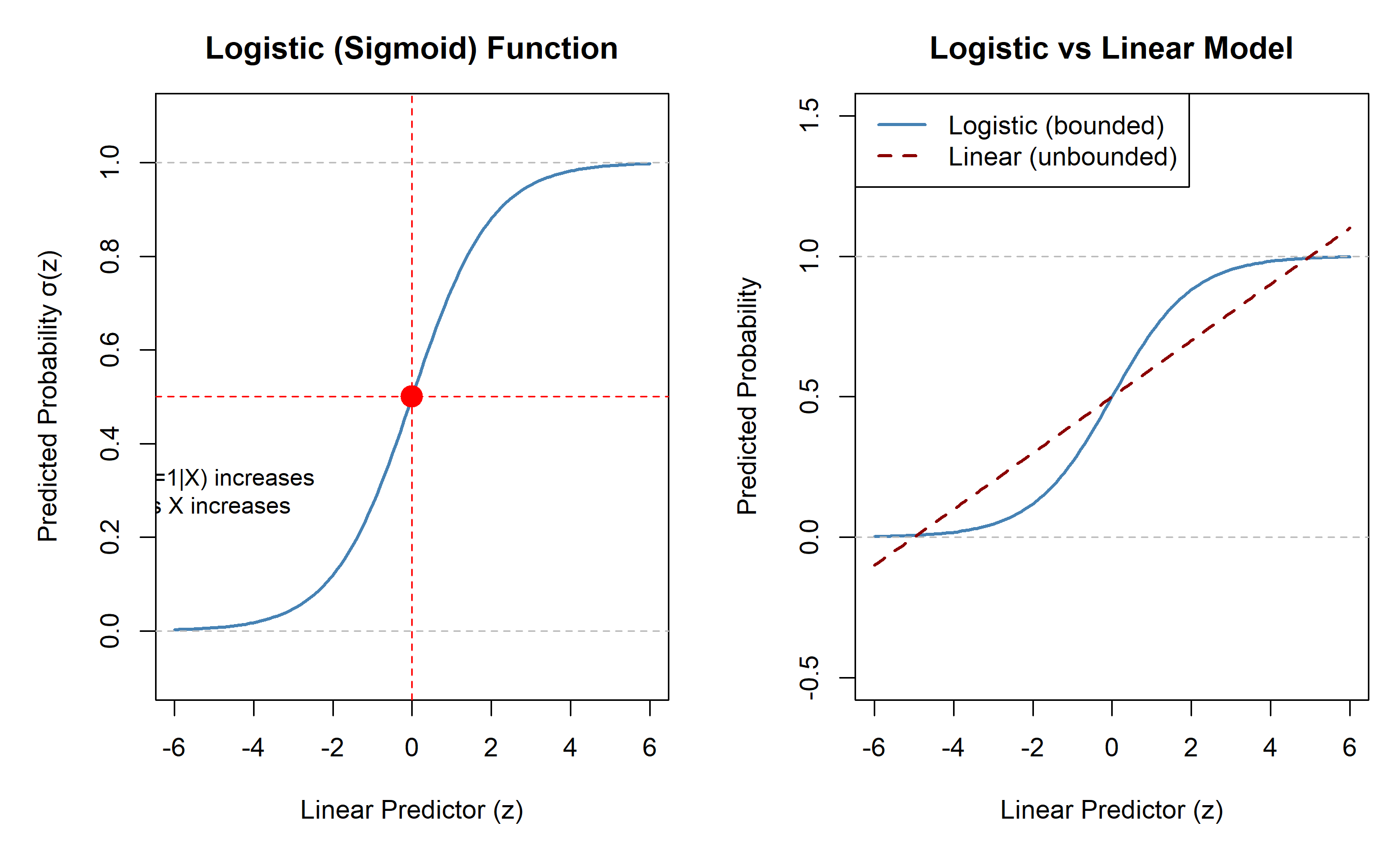
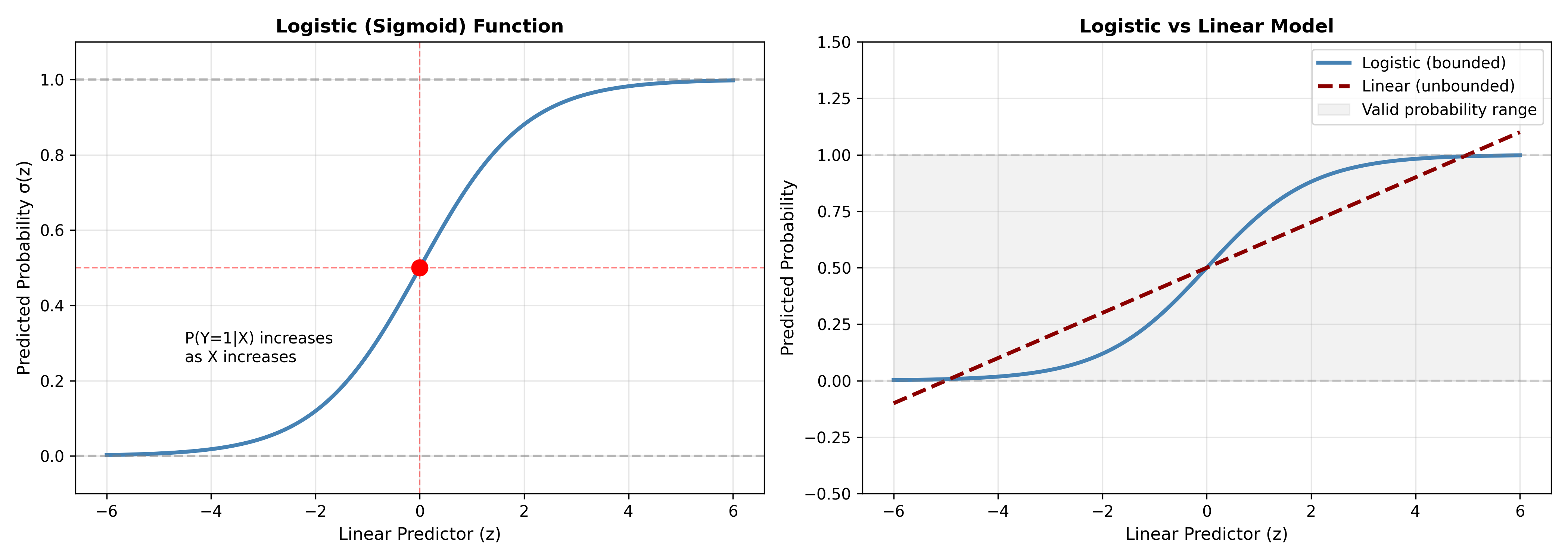
The **logistic function (sigmoid)** maps any real number to (0, 1):
$$\sigma(z) = \frac{1}{1 + e^{-z}}$$
where z is the **linear predictor**: $z = \beta_0 + \beta_1 X_1 + \cdots + \beta_p X_p$
::: {.callout-tip icon="false"}
## 🔑 Key Formula: The Logistic (Sigmoid) Function
$$\sigma(z) = \frac{1}{1 + e^{-z}} = \frac{e^z}{1 + e^z}$$
**Properties:**
- σ(z) ∈ (0, 1) for all z ∈ ℝ
- σ(0) = 0.5
- σ(z) is monotonically increasing
- As z → ∞, σ(z) → 1; as z → −∞, σ(z) → 0
- Derivative: σ'(z) = σ(z)[1 − σ(z)]
:::
### Visualisation and Intuition
::: {.panel-tabset}
## R
```{r}
library(tidyverse)

# Plot logistic function
z_values <- seq(-6, 6, by = 0.1)
sigma_values <- 1 / (1 + exp(-z_values))

par(mfrow = c(1, 2), mar = c(5, 5, 3, 1))

# Plot 1: Logistic function
plot(z_values, sigma_values, type = "l", lwd = 2, col = "steelblue",
     xlab = "Linear Predictor (z)", ylab = "Predicted Probability σ(z)",
     main = "Logistic (Sigmoid) Function",
     ylim = c(-0.1, 1.1))
abline(h = 0, col = "gray", lty = 2)
abline(h = 1, col = "gray", lty = 2)
abline(h = 0.5, col = "red", lty = 2, lwd = 1)
abline(v = 0, col = "red", lty = 2, lwd = 1)
points(0, 0.5, pch = 16, cex = 2, col = "red")
text(-5, 0.3, "P(Y=1|X) increases\nas X increases", cex = 0.9)

# Plot 2: Comparison with linear regression
plot(z_values, sigma_values, type = "l", lwd = 2, col = "steelblue",
     xlab = "Linear Predictor (z)", ylab = "Predicted Probability",
     main = "Logistic vs Linear Model",
     ylim = c(-0.5, 1.5))
abline(h = 0, col = "gray", lty = 2)
abline(h = 1, col = "gray", lty = 2)
# Add linear model
linear_pred <- 0.5 + 0.1 * z_values
lines(z_values, linear_pred, lwd = 2, col = "darkred", lty = 2)
legend("topleft", legend = c("Logistic (bounded)", "Linear (unbounded)"),
       col = c("steelblue", "darkred"), lwd = 2, lty = c(1, 2))
par(mfrow = c(1, 1))
```
## Python
```{python}
import numpy as np
import matplotlib.pyplot as plt
# Logistic function
def sigmoid(z):
return 1 / (1 + np.exp(-z))
z_values = np.linspace(-6, 6, 200)
sigma_values = sigmoid(z_values)
linear_values = 0.5 + 0.1 * z_values
fig, axes = plt.subplots(1, 2, figsize=(14, 5))
# Plot 1: Logistic function
ax = axes[0]
ax.plot(z_values, sigma_values, linewidth=2.5, color='steelblue', label='σ(z)')
ax.axhline(0, color='gray', linestyle='--', alpha=0.5)
ax.axhline(1, color='gray', linestyle='--', alpha=0.5)
ax.axhline(0.5, color='red', linestyle='--', linewidth=1, alpha=0.5)
ax.axvline(0, color='red', linestyle='--', linewidth=1, alpha=0.5)
ax.plot(0, 0.5, 'ro', markersize=10)
ax.set_xlabel('Linear Predictor (z)', fontsize=11)
ax.set_ylabel('Predicted Probability σ(z)', fontsize=11)
ax.set_title('Logistic (Sigmoid) Function', fontsize=12, fontweight='bold')
ax.set_ylim([-0.1, 1.1])
ax.grid(True, alpha=0.3)
ax.text(-4.5, 0.25, 'P(Y=1|X) increases\nas X increases', fontsize=10)
# Plot 2: Comparison
ax = axes[1]
ax.plot(z_values, sigma_values, linewidth=2.5, color='steelblue', label='Logistic (bounded)')
ax.plot(z_values, linear_values, linewidth=2.5, color='darkred', linestyle='--', label='Linear (unbounded)')
ax.axhline(0, color='gray', linestyle='--', alpha=0.3)
ax.axhline(1, color='gray', linestyle='--', alpha=0.3)
ax.fill_between(z_values, 0, 1, alpha=0.1, color='gray', label='Valid probability range')
ax.set_xlabel('Linear Predictor (z)', fontsize=11)
ax.set_ylabel('Predicted Probability', fontsize=11)
ax.set_title('Logistic vs Linear Model', fontsize=12, fontweight='bold')
ax.set_ylim([-0.5, 1.5])
ax.grid(True, alpha=0.3)
ax.legend(fontsize=10)
plt.tight_layout()
plt.savefig('sigmoid_function.png', dpi=300, bbox_inches='tight')
plt.show()
```
:::
::: {.callout-caution icon="false"}
## 📝 Section 13.2 Review Questions
1. Verify: σ(0) = 0.5. What does this mean in terms of equal odds?
2. What is σ(−3)? σ(3)? How do they relate?
3. Why is the logistic function preferable to a linear function for classification?
:::
## The Logistic Regression Model
**Logistic regression** models the probability of the positive class using the logistic function:
$$P(Y = 1 | X) = \sigma(\beta_0 + \beta_1 X_1 + \cdots + \beta_p X_p)$$
### Interpreting Coefficients: Odds and Odds Ratios
The **odds** of success are:
$$\text{Odds} = \frac{P(Y = 1)}{P(Y = 0)} = \frac{P(Y = 1)}{1 - P(Y = 1)}$$
The **log-odds (logit)** are:
$$\text{log(Odds)} = \log\left(\frac{P(Y = 1)}{1 - P(Y = 1)}\right) = \beta_0 + \beta_1 X_1 + \cdots + \beta_p X_p$$
For a one-unit increase in X_j:
$$\text{log(Odds)}_{\text{new}} - \text{log(Odds)}_{\text{old}} = \beta_j$$
Taking the exponential:
$$\frac{\text{Odds}_{\text{new}}}{\text{Odds}_{\text{old}}} = e^{\beta_j}$$
The **odds ratio** is $e^{\beta_j}$: a one-unit increase in X_j **multiplies the odds by** $e^{\beta_j}$.
::: {.callout-tip icon="false"}
## 🔑 Key Formula: Coefficient Interpretation
For a logistic regression coefficient β_j:
**Odds ratio:** $OR_j = e^{\beta_j}$
**Interpretation:**
- If β_j = 0, OR_j = 1 (no effect)
- If β_j > 0, OR_j > 1 (increases odds)
- If β_j < 0, OR_j < 1 (decreases odds)
**Example:** If β_age = 0.05, then e^{0.05} = 1.051
- A one-year increase in age multiplies the odds by 1.051
- Per 10-year increase: odds are multiplied by e^{0.5} ≈ 1.649
:::
### Worked Example: Credit Default Logistic Regression
::: {.panel-tabset}
## R
```{r}
library(tidyverse)
# Simulate credit default data
set.seed(42)
n <- 1000
age <- rnorm(n, mean = 45, sd = 15)
income <- rlnorm(n, meanlog = 11, sdlog = 0.8)
credit_utilisation <- rbeta(n, 2, 5)
credit_score <- 850 - 5 * age + 0.0001 * income + 300 * credit_utilisation + rnorm(n, 0, 100)
# Probability of default
true_linear_pred <- -8 + 0.03 * age - 0.0000005 * income - 0.02 * credit_score
prob_default <- 1 / (1 + exp(-true_linear_pred))
default <- rbinom(n, 1, prob_default)
credit_data <- tibble(
age, income, credit_utilisation, credit_score, default
)
# Fit logistic regression
fit_logistic <- glm(default ~ age + log(income) + credit_utilisation + credit_score,
data = credit_data, family = binomial(link = "logit"))
summary(fit_logistic)
# Extract coefficients and odds ratios
coefs <- coef(fit_logistic)
odds_ratios <- exp(coefs)
cat("\n\nCoefficient Interpretation (Odds Ratios):\n\n")
for (i in 2:length(coefs)) {
var_name <- names(coefs)[i]
coef_val <- coefs[i]
or_val <- odds_ratios[i]
cat(var_name, ":\n")
cat(" Coefficient (β):", round(coef_val, 6), "\n")
cat(" Odds Ratio (e^β):", round(or_val, 4), "\n")
if (or_val > 1) {
pct_increase <- (or_val - 1) * 100
cat(" → One-unit increase multiplies odds by", round(or_val, 4),
"(", round(pct_increase, 1), "% increase)\n\n")
} else {
pct_decrease <- (1 - or_val) * 100
cat(" → One-unit increase multiplies odds by", round(or_val, 4),
"(", round(pct_decrease, 1), "% decrease)\n\n")
}
}
# Predicted probabilities for specific cases
new_cases <- tibble(
age = c(30, 50),
income = c(30000, 100000),
credit_utilisation = c(0.3, 0.7),
credit_score = c(750, 600)
)
preds <- predict(fit_logistic, newdata = new_cases, type = "response")
cat("Predicted Default Probabilities:\n\n")
for (i in 1:nrow(new_cases)) {
cat("Applicant", i, ":\n")
cat(" Age:", new_cases$age[i], "\n")
cat(" Income: $", new_cases$income[i], "\n")
cat(" Credit Utilisation:", new_cases$credit_utilisation[i], "\n")
cat(" Credit Score:", new_cases$credit_score[i], "\n")
cat(" Predicted Default Probability:", round(preds[i], 4), " (",
round(preds[i] * 100, 2), "%)\n\n")
}
```
## Python
```{python}
import numpy as np
import pandas as pd
import matplotlib.pyplot as plt
from sklearn.linear_model import LogisticRegression
import statsmodels.api as sm
np.random.seed(42)
n = 1000
age = np.random.normal(45, 15, n)
income = np.exp(np.random.normal(11, 0.8, n))
credit_util = np.random.beta(2, 5, n)
credit_score = 850 - 5*age + 0.0001*income + 300*credit_util + np.random.normal(0, 100, n)
# Probability of default
true_linear_pred = -8 + 0.03*age - 0.0000005*income - 0.02*credit_score
prob_default = 1 / (1 + np.exp(-true_linear_pred))
default = np.random.binomial(1, prob_default, n)
credit_data = pd.DataFrame({
'age': age,
'income': income,
'credit_util': credit_util,
'credit_score': credit_score,
'default': default
})
# Fit logistic regression using statsmodels for detailed output
X = credit_data[['age', 'credit_util', 'credit_score']].copy()
X['log_income'] = np.log(credit_data['income'])
X = sm.add_constant(X)
y = credit_data['default']
fit_logistic = sm.Logit(y, X).fit()
print(fit_logistic.summary())
# Coefficient interpretation
print("\n\nCoefficient Interpretation (Odds Ratios):\n")
coefs = fit_logistic.params[1:] # Exclude intercept
odds_ratios = np.exp(coefs)
for var, coef_val, or_val in zip(coefs.index, coefs.values, odds_ratios.values):
print(f"{var}:")
print(f" Coefficient (β): {coef_val:.6f}")
print(f" Odds Ratio (e^β): {or_val:.4f}")
if or_val > 1:
pct_change = (or_val - 1) * 100
print(f" → One-unit increase multiplies odds by {or_val:.4f} ({pct_change:.1f}% increase)\n")
else:
pct_change = (1 - or_val) * 100
print(f" → One-unit increase multiplies odds by {or_val:.4f} ({pct_change:.1f}% decrease)\n")
# Predicted probabilities
new_cases = pd.DataFrame({
'const': 1,
'age': [30, 50],
'credit_util': [0.3, 0.7],
'credit_score': [750, 600],
'log_income': [np.log(30000), np.log(100000)]
})
new_cases = new_cases[['const', 'age', 'credit_util', 'credit_score', 'log_income']]
preds = fit_logistic.predict(new_cases)
print("Predicted Default Probabilities:\n")
for i in range(len(preds)):
print(f"Applicant {i+1}:")
print(f" Age: {new_cases.iloc[i]['age']:.0f}")
print(f" Income: ${np.exp(new_cases.iloc[i]['log_income']):,.0f}")
print(f" Credit Utilisation: {new_cases.iloc[i]['credit_util']:.1f}")
print(f" Credit Score: {new_cases.iloc[i]['credit_score']:.0f}")
print(f" Predicted Default Probability: {preds.iloc[i]:.4f} ({preds.iloc[i]*100:.2f}%)\n")
```
:::
::: {.callout-caution icon="false"}
## 📝 Section 13.3 Review Questions
1. If β_age = 0.03, what is the odds ratio? Interpret it.
2. If β_credit_score = −0.02, what happens to default odds when credit score increases by 50 points?
3. Why is the log-odds (logit) linear in X, but the probability is nonlinear?
4. Can a coefficient in logistic regression be interpreted as "change in probability per unit change in X"? Why or why not?
:::
## Maximum Likelihood Estimation (MLE)
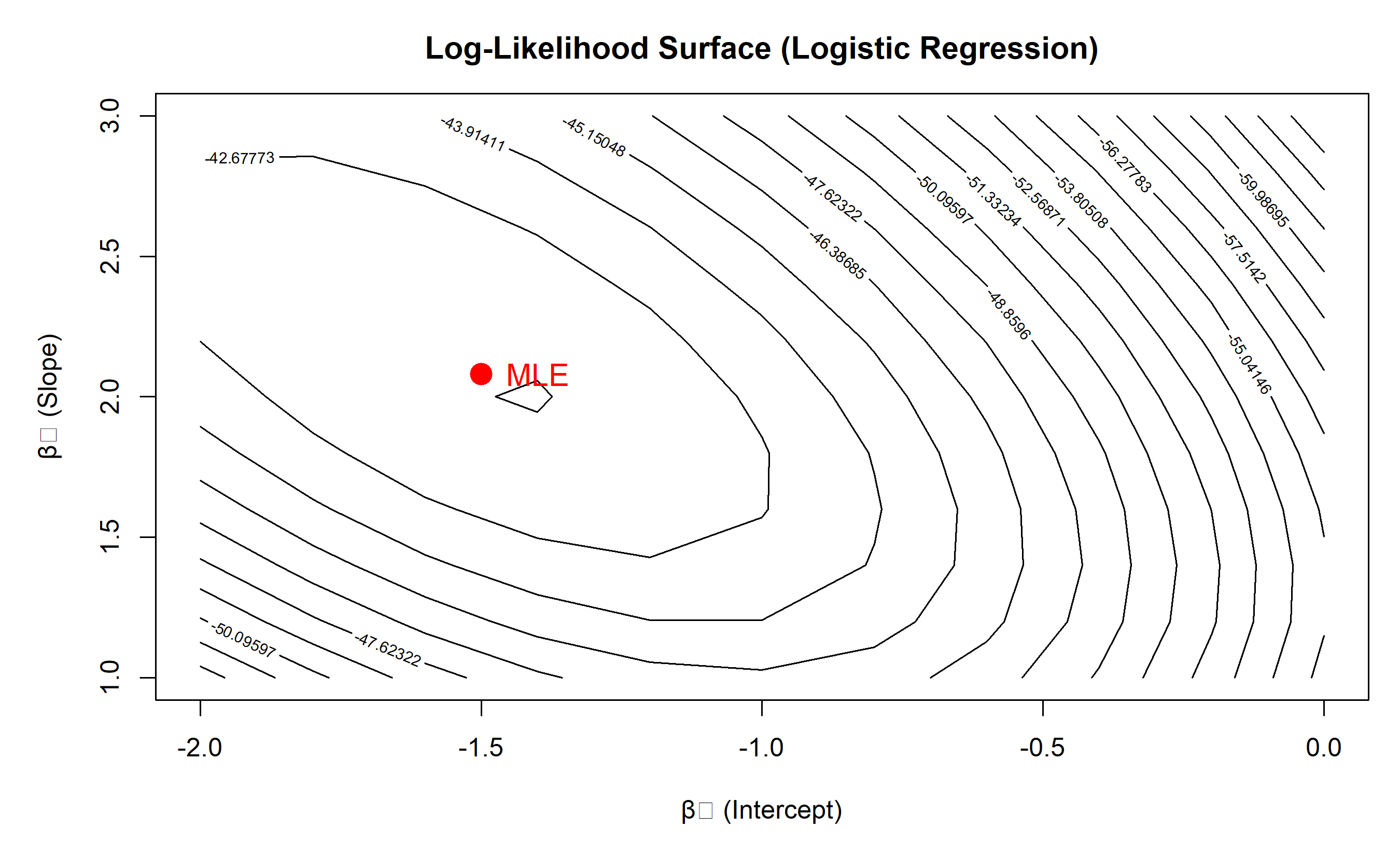
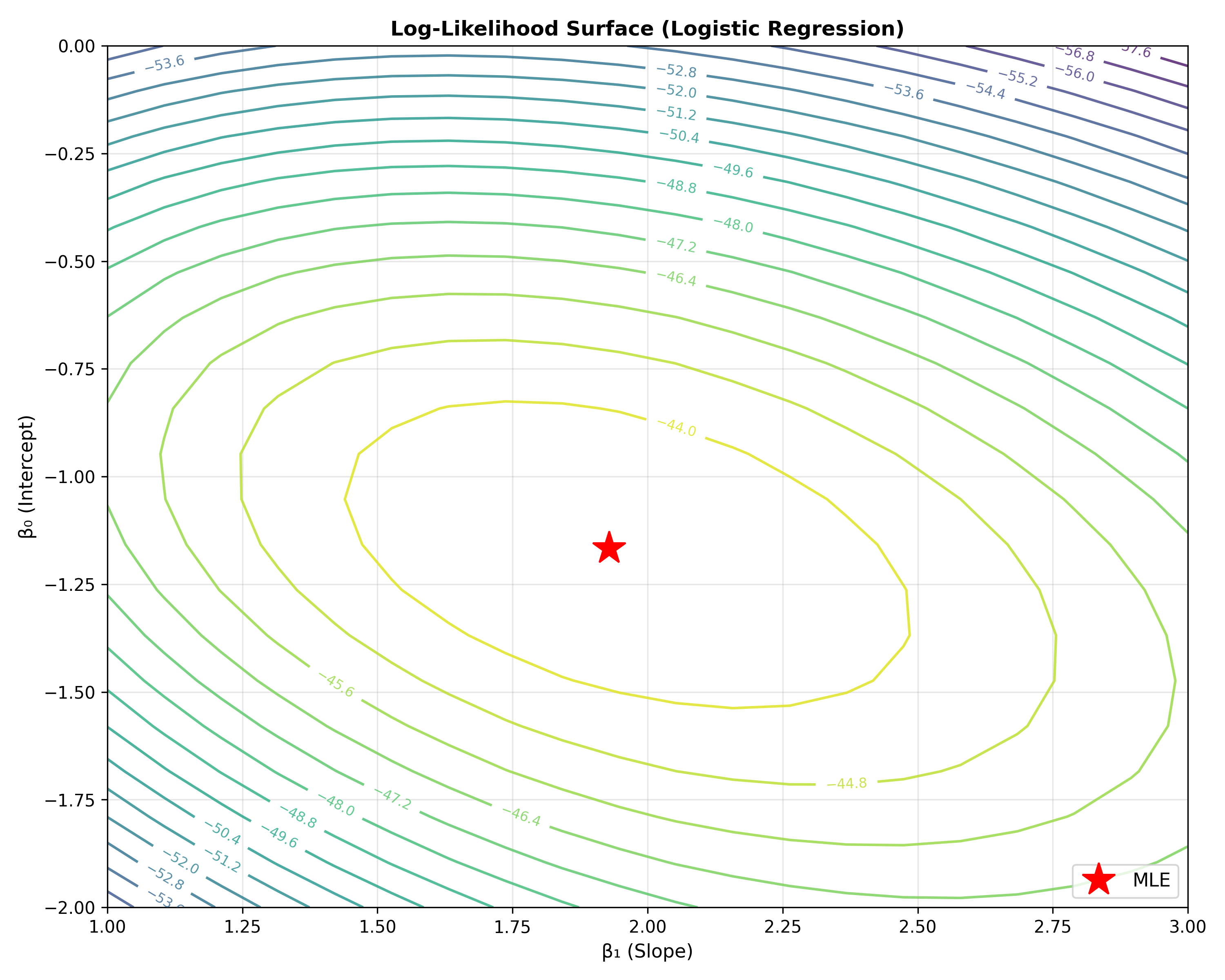
Unlike OLS, logistic regression coefficients are estimated using **maximum likelihood estimation (MLE)**, not closed-form formulas.
::: {.callout-note icon="false"}
## 📘 Theory: MLE for Logistic Regression
**Likelihood function:** For observed data (y_i, x_i), the likelihood of observing y_i given x_i is:
$$L(\beta) = \prod_{i=1}^{n} p_i^{y_i} (1 - p_i)^{1 - y_i}$$
where $p_i = \sigma(\beta_0 + \beta_1 x_{i,1} + \cdots + \beta_p x_{i,p})$
**Log-likelihood:**
$$\ell(\beta) = \sum_{i=1}^{n} [y_i \log(p_i) + (1 - y_i) \log(1 - p_i)]$$
**Goal:** Find β that **maximises** ℓ(β) (not minimises, unlike OLS).
**Method:** Gradient ascent (or iteratively reweighted least squares, IRLS):
1. Start with initial guess β^(0)
2. Compute gradient: ∇ℓ(β^(t))
3. Update: β^(t+1) = β^(t) + α ∇ℓ(β^(t))
4. Repeat until convergence
**Properties:**
- No closed-form solution (unlike OLS)
- Converges under mild conditions
- Coefficients are asymptotically normal (allows confidence intervals and hypothesis tests)
:::
### Worked Example: Computing Log-Likelihood
::: {.panel-tabset}
## R
```{r}
# Compute log-likelihood manually for a simple logistic regression

# Generate simple data
set.seed(42)
n <- 100
x <- rnorm(n, 0, 1)
true_beta <- c(-1, 2)  # Intercept, slope
p <- 1 / (1 + exp(-(true_beta[1] + true_beta[2] * x)))
y <- rbinom(n, 1, p)

# Log-likelihood function
log_likelihood <- function(beta, x, y) {
  p <- 1 / (1 + exp(-(beta[1] + beta[2] * x)))
  # Avoid log(0) by bounding p
  p <- pmax(pmin(p, 1 - 1e-10), 1e-10)
  sum(y * log(p) + (1 - y) * log(1 - p))
}

# Grid search over beta values
beta0_seq <- seq(-2, 0, by = 0.2)
beta1_seq <- seq(1, 3, by = 0.2)
ll_grid <- matrix(NA, length(beta0_seq), length(beta1_seq))

for (i in seq_along(beta0_seq)) {
  for (j in seq_along(beta1_seq)) {
    ll_grid[i, j] <- log_likelihood(c(beta0_seq[i], beta1_seq[j]), x, y)
  }
}

# Plot log-likelihood surface
par(mar = c(5, 5, 3, 1))
contour(beta0_seq, beta1_seq, ll_grid,
        xlab = "β₀ (Intercept)", ylab = "β₁ (Slope)",
        main = "Log-Likelihood Surface (Logistic Regression)",
        levels = seq(min(ll_grid), max(ll_grid), length.out = 20),
        drawlabels = TRUE)

# Mark MLE (fit logistic regression for comparison)
fit <- glm(y ~ x, family = binomial(link = "logit"))
mle_beta <- coef(fit)
points(mle_beta[1], mle_beta[2], pch = 16, cex = 2, col = "red")
text(mle_beta[1] + 0.1, mle_beta[2], "MLE", col = "red", cex = 1.2)
cat("MLE (from glm):\n")
cat("β₀:", round(mle_beta[1], 4), "\n")
cat("β₁:", round(mle_beta[2], 4), "\n")
cat("Log-likelihood at MLE:", round(log_likelihood(mle_beta, x, y), 2), "\n")
```
## Python
```{python}
import numpy as np
from scipy.optimize import minimize
import matplotlib.pyplot as plt

# Generate simple data
np.random.seed(42)
n = 100
x = np.random.normal(0, 1, n)
true_beta = np.array([-1, 2])
p = 1 / (1 + np.exp(-(true_beta[0] + true_beta[1] * x)))
y = np.random.binomial(1, p, n)

# Log-likelihood function (we'll minimise negative log-likelihood)
def neg_log_likelihood(beta, x, y):
    p = 1 / (1 + np.exp(-(beta[0] + beta[1] * x)))
    p = np.clip(p, 1e-10, 1 - 1e-10)
    return -np.sum(y * np.log(p) + (1 - y) * np.log(1 - p))

# Grid search
beta0_seq = np.linspace(-2, 0, 20)
beta1_seq = np.linspace(1, 3, 20)
ll_grid = np.zeros((len(beta0_seq), len(beta1_seq)))

for i, b0 in enumerate(beta0_seq):
    for j, b1 in enumerate(beta1_seq):
        ll_grid[i, j] = -neg_log_likelihood(np.array([b0, b1]), x, y)

# Find MLE numerically
result = minimize(neg_log_likelihood, x0=[0, 0], args=(x, y), method='BFGS')
mle_beta = result.x

# Plot
fig, ax = plt.subplots(figsize=(10, 8))
contour = ax.contour(beta1_seq, beta0_seq, ll_grid,
                      levels=20, cmap='viridis', alpha=0.8)
ax.clabel(contour, inline=True, fontsize=8)
ax.plot(mle_beta[1], mle_beta[0], 'r*', markersize=20, label='MLE')
ax.set_xlabel('β₁ (Slope)', fontsize=11)
ax.set_ylabel('β₀ (Intercept)', fontsize=11)
ax.set_title('Log-Likelihood Surface (Logistic Regression)', fontsize=12, fontweight='bold')
ax.legend(fontsize=11)
ax.grid(True, alpha=0.3)

plt.tight_layout()
plt.savefig('logistic_mle_surface.png', dpi=300, bbox_inches='tight')
plt.show()
print("MLE (from numerical optimisation):")
print(f"β₀: {mle_beta[0]:.4f}")
print(f"β₁: {mle_beta[1]:.4f}")
print(f"Negative log-likelihood at MLE: {neg_log_likelihood(mle_beta, x, y):.2f}")
# Compare with sklearn
from sklearn.linear_model import LogisticRegression
X = x.reshape(-1, 1)
lr = LogisticRegression(fit_intercept=True)
lr.fit(X, y)
print(f"\nsklearn LogisticRegression:")
print(f"β₀: {lr.intercept_[0]:.4f}")
print(f"β₁: {lr.coef_[0, 0]:.4f}")
```
:::
::: {.callout-caution icon="false"}
## 📝 Section 13.4 Review Questions
1. Why can't logistic regression be solved with a closed-form formula like OLS?
2. What does maximising log-likelihood achieve?
3. In the log-likelihood formula, why do we include both y_i log(p_i) and (1−y_i) log(1−p_i)?
4. How do confidence intervals for logistic regression coefficients differ from OLS?
:::
## Interpreting Logistic Regression Output
Standard software (R's `glm`, Python's `statsmodels`) provides comprehensive output:
::: {.panel-tabset}
## R
```{r}
# Full logistic regression output interpretation
set.seed(42)
n <- 200
age <- rnorm(n, 50, 15)
debt_to_income <- rbeta(n, 2, 5)
employment_years <- rpois(n, 10)
# Default probability
p_default <- 0.05 + 0.003 * age + 0.3 * debt_to_income - 0.02 * employment_years
p_default <- pmax(pmin(p_default, 0.99), 0.01)
default <- rbinom(n, 1, p_default)
credit_data <- data.frame(age, debt_to_income, employment_years, default)
fit <- glm(default ~ age + debt_to_income + employment_years,
data = credit_data, family = binomial(link = "logit"))
summary(fit)
# Extract key statistics
cat("\n\n=== INTERPRETING THE OUTPUT ===\n\n")
# Coefficients
coefs_summary <- summary(fit)$coefficients
cat("Coefficients:\n")
print(coefs_summary)
cat("\n\nPseudo-R² Measures:\n")
cat("McFadden R²:", round(1 - fit$deviance / fit$null.deviance, 4), "\n")
cat("(Logistic regression has no single R² like OLS; McFadden R² is an analogue)\n\n")
# Model significance (overall)
cat("Model Significance (Likelihood Ratio Test):\n")
cat("Null deviance:", round(fit$null.deviance, 2), " (model with intercept only)\n")
cat("Residual deviance:", round(fit$deviance, 2), " (full model)\n")
cat("Likelihood ratio test statistic:", round(fit$null.deviance - fit$deviance, 2), "\n")
cat("p-value:", round(1 - pchisq(fit$null.deviance - fit$deviance, fit$df.residual - fit$df.null), 4), "\n")
cat("(If p < 0.05, the model is significantly better than intercept-only)\n\n")
# Predicted probabilities and calibration
pred_prob <- predict(fit, type = "response")
pred_label <- ifelse(pred_prob > 0.5, 1, 0)
cat("Calibration:\n")
cat("Average predicted probability:", round(mean(pred_prob), 4), "\n")
cat("Observed event rate (proportion of defaults):", round(mean(default), 4), "\n")
cat("(These should be similar for well-calibrated models)\n")
```
## Python
```{python}
import statsmodels.api as sm
import numpy as np
from sklearn.metrics import roc_auc_score
np.random.seed(42)
n = 200
age = np.random.normal(50, 15, n)
debt_to_income = np.random.beta(2, 5, n)
employment_years = np.random.poisson(10, n)
# Default probability
p_default = 0.05 + 0.003*age + 0.3*debt_to_income - 0.02*employment_years
p_default = np.clip(p_default, 0.01, 0.99)
default = np.random.binomial(1, p_default, n)
# Fit using statsmodels
X = np.column_stack([age, debt_to_income, employment_years])
X = sm.add_constant(X)
y = default
logit_model = sm.Logit(y, X).fit()
print(logit_model.summary())
# Pseudo-R² (McFadden)
print(f"\n\nPseudo-R² (McFadden): {logit_model.prsquared:.4f}")
print("(Logistic regression has no single R² like OLS; McFadden R² is an analogue)")
# Model significance
print(f"\nModel Significance (Likelihood Ratio Test):")
print(f"Log-Likelihood (full model): {logit_model.llf:.2f}")
print(f"Log-Likelihood (intercept-only): {logit_model.llnull:.2f}")
lr_stat = 2 * (logit_model.llf - logit_model.llnull)
print(f"LR test statistic: {lr_stat:.2f}")
print(f"p-value: {logit_model.llr_pvalue:.4f}")
# Predictions and calibration
pred_prob = logit_model.predict(X)
print(f"\nCalibration:")
print(f"Average predicted probability: {pred_prob.mean():.4f}")
print(f"Observed event rate: {y.mean():.4f}")
print(f"(These should be similar for well-calibrated models)")
# AUC
auc = roc_auc_score(y, pred_prob)
print(f"\nModel Discrimination (AUC): {auc:.4f}")
```
:::
### Key Metrics and Pseudo-R² Measures
Unlike OLS, logistic regression has no single R². Common pseudo-R² measures:
| Metric | Formula | Interpretation |
|---|---|---|
| **McFadden R²** | 1 − log(L) / log(L₀) | Higher is better; 0.2–0.4 is good |
| **Nagelkerke R²** | R² / (1 − L₀^{2/n}) | Scaled to 0–1; similar to OLS R² |
| **AUC** | See Chapter 12 | Discrimination ability; 0.7–0.8 is good |
::: {.callout-caution icon="false"}
## 📝 Section 13.5 Review Questions
1. What does McFadden R² = 0.25 tell you about model fit?
2. Why is AUC sometimes more informative than McFadden R² for logistic regression?
3. If average predicted probability (0.15) differs from observed event rate (0.20), what does this suggest?
4. How would you test whether a coefficient is statistically significant in logistic regression?
:::
## Regularised Logistic Regression
Like linear regression, logistic regression can overfit with many correlated predictors. **L1 and L2 regularisation** (Chapter 10) extend directly to logistic regression.
::: {.callout-note icon="false"}
## 📘 Theory: Regularised Logistic Regression
**Objective:**
$$\ell(\beta) - \lambda \left[ (1 - \alpha) \frac{1}{2} \sum \beta_j^2 + \alpha \sum |\beta_j| \right]$$
- α = 0: Ridge (L2) — shrinks coefficients toward zero, all retained
- α = 1: Lasso (L1) — sparse solution, some coefficients zero
- α ∈ (0, 1): Elastic Net — combination
**When to use:**
- Many correlated predictors → Ridge or Elastic Net
- Want sparse model → Lasso
- High-dimensional data (p >> n) → Regularisation is essential
:::
### Worked Example: Regularised Logistic Regression
::: {.panel-tabset}
## R
```{r}
library(glmnet)
# Generate credit data with many correlated features
set.seed(42)
n <- 200
p <- 30
X <- matrix(rnorm(n * p), nrow = n, ncol = p)
# Introduce correlations
for (j in 2:p) {
X[, j] <- 0.7 * X[, j] + 0.3 * X[, j - 1] + rnorm(n, 0, 0.2)
}
# Outcome: true signal from first 3 features only
y <- rbinom(n, 1, prob = 1 / (1 + exp(-(X[, 1] - 0.5 * X[, 2] + 0.3 * X[, 3]))))
# Standardise
X_scaled <- scale(X)
# Ridge logistic regression
ridge_cv <- cv.glmnet(X_scaled, y, alpha = 0, family = "binomial", nfolds = 5)
cat("Ridge Logistic Regression:\n")
cat("Optimal λ:", round(ridge_cv$lambda.min, 4), "\n")
cat("CV error at optimal λ:", round(min(ridge_cv$cvm), 4), "\n\n")
# Lasso logistic regression
lasso_cv <- cv.glmnet(X_scaled, y, alpha = 1, family = "binomial", nfolds = 5)
cat("Lasso Logistic Regression:\n")
cat("Optimal λ:", round(lasso_cv$lambda.min, 4), "\n")
cat("CV error at optimal λ:", round(min(lasso_cv$cvm), 4), "\n")
cat("Number of non-zero coefficients:", sum(coef(glmnet(X_scaled, y, alpha = 1, lambda = lasso_cv$lambda.min, family = "binomial")) != 0) - 1, "\n\n")
# Elastic Net
en_cv <- cv.glmnet(X_scaled, y, alpha = 0.5, family = "binomial", nfolds = 5)
cat("Elastic Net Logistic Regression (α=0.5):\n")
cat("Optimal λ:", round(en_cv$lambda.min, 4), "\n")
cat("CV error at optimal λ:", round(min(en_cv$cvm), 4), "\n")
cat("Number of non-zero coefficients:", sum(coef(glmnet(X_scaled, y, alpha = 0.5, lambda = en_cv$lambda.min, family = "binomial")) != 0) - 1, "\n\n")
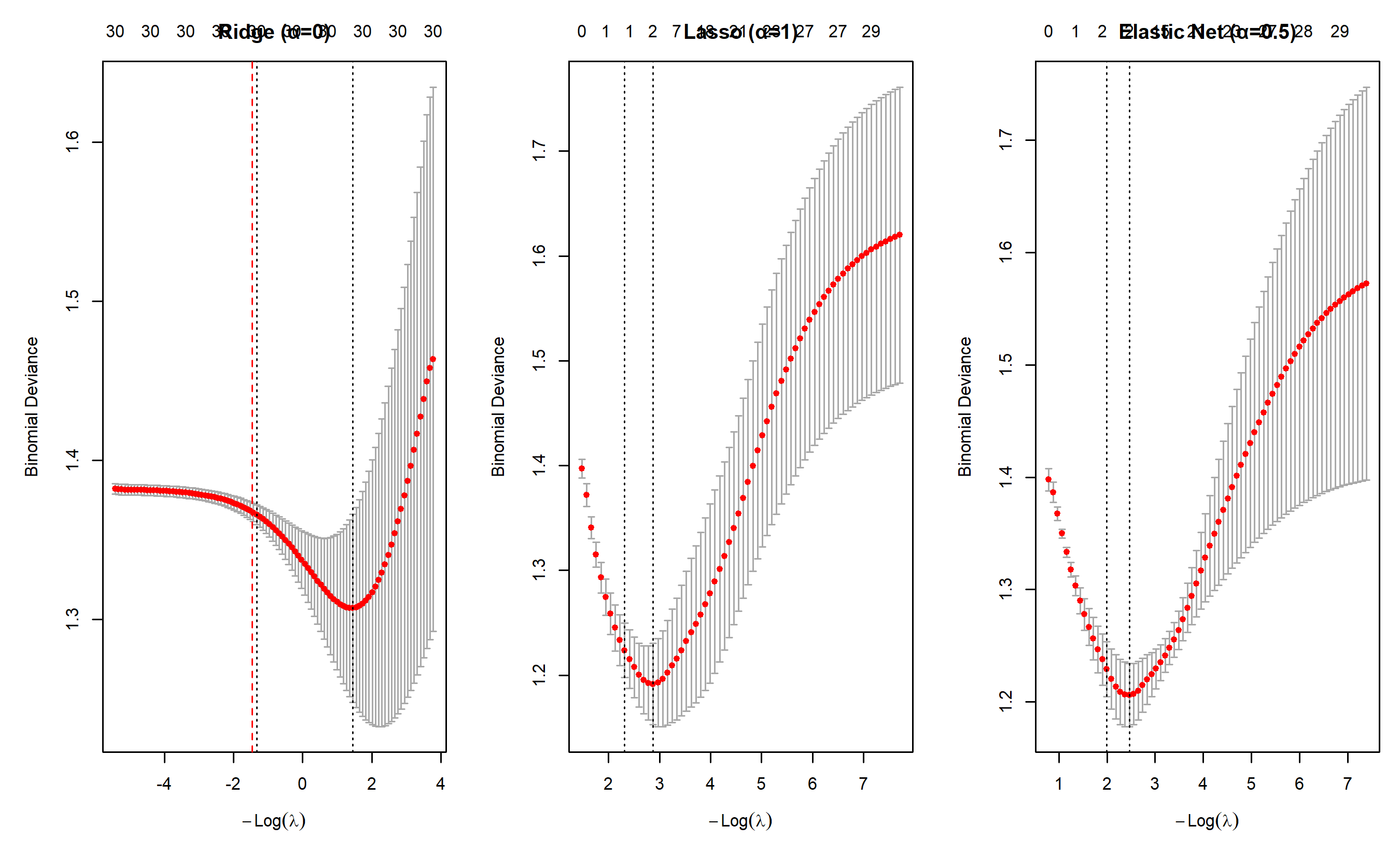
# Plot coefficient paths
par(mfrow = c(1, 3), mar = c(5, 5, 3, 1))
plot(ridge_cv, main = "Ridge (α=0)")
abline(v = log(ridge_cv$lambda.min), col = "red", lty = 2)
plot(lasso_cv, main = "Lasso (α=1)")
abline(v = log(lasso_cv$lambda.min), col = "red", lty = 2)
plot(en_cv, main = "Elastic Net (α=0.5)")
abline(v = log(en_cv$lambda.min), col = "red", lty = 2)
par(mfrow = c(1, 1))
```
## Python
```{python}
from sklearn.linear_model import LogisticRegression
from sklearn.preprocessing import StandardScaler
import numpy as np

np.random.seed(42)
n = 200
p = 30

X = np.random.normal(0, 1, (n, p))
# Introduce correlations
for j in range(1, p):
    X[:, j] = 0.7 * X[:, j] + 0.3 * X[:, j-1] + np.random.normal(0, 0.2, n)

# Outcome
y = (np.random.random(n) < 1 / (1 + np.exp(-(X[:, 0] - 0.5*X[:, 1] + 0.3*X[:, 2])))).astype(int)

# Standardise
scaler = StandardScaler()
X_scaled = scaler.fit_transform(X)

# Ridge
ridge = LogisticRegression(penalty='l2', C=1.0, solver='lbfgs', max_iter=1000)
ridge.fit(X_scaled, y)
print(f"Ridge Logistic Regression:")
print(f" Coefficients: {np.sum(ridge.coef_ != 0)} non-zero (all 30)")
print(f" Training accuracy: {ridge.score(X_scaled, y):.4f}\n")
# Lasso
lasso = LogisticRegression(penalty='l1', C=1.0, solver='saga', max_iter=1000)
lasso.fit(X_scaled, y)
print(f"Lasso Logistic Regression:")
print(f" Non-zero coefficients: {np.sum(lasso.coef_ != 0)} / 30")
print(f" Training accuracy: {lasso.score(X_scaled, y):.4f}\n")
# Elastic Net
from sklearn.linear_model import SGDClassifier
en = SGDClassifier(loss='log_loss', penalty='elasticnet', l1_ratio=0.5,
alpha=0.0001, max_iter=1000, random_state=42)
en.fit(X_scaled, y)
print(f"Elastic Net Logistic Regression (α=0.5):")
print(f" Non-zero coefficients: {np.sum(en.coef_ != 0)} / 30")
print(f" Training accuracy: {en.score(X_scaled, y):.4f}")
```
:::
::: {.callout-caution icon="false"}
## 📝 Section 13.6 Review Questions
1. Why might Lasso be preferable to Ridge for a credit scoring model with 50 features?
2. If Lasso selects only 8 features, is this enough to build a reliable model? What additional checks are needed?
:::
## Building a Credit Risk Scorecard
A **credit scorecard** translates logistic regression coefficients into a points-based system usable by loan officers.
::: {.callout-note icon="false"}
## 📘 Theory: Scorecard Construction
1. **Weight of Evidence (WOE):** For a variable X with categories (or binned continuous values), WOE measures how well the category discriminates good vs bad borrowers:
$$\text{WOE}_i = \ln\left( \frac{\% \text{ Good}_i}{\% \text{ Bad}_i} \right)$$
where % Good_i and % Bad_i are the percentages of good/bad borrowers in category i.
2. **Information Value (IV):** Measures total discriminatory power of a variable:
$$\text{IV} = \sum_i (\% \text{Good}_i - \% \text{Bad}_i) \times \text{WOE}_i$$
- IV < 0.02: weak predictor
- 0.02 < IV < 0.1: moderate predictor
- 0.1 < IV < 0.3: strong predictor
- IV > 0.3: very strong predictor
3. **Points transformation:** Map WOE to points such that odds double for every X points:
$$\text{Points} = \text{Scaling Factor} \times \text{WOE} + \text{Offset}$$
The scaling factor ensures a doubling of odds corresponds to a fixed points increase (commonly 20–50 points).
:::
### Worked Example: Credit Scorecard
::: {.panel-tabset}
## R
```{r}
# Build a credit risk scorecard using logistic regression
set.seed(42)
n <- 500
# Binary outcome
default <- rbinom(n, 1, 0.15)
# Continuous variable: credit score (strong predictor)
credit_score <- rnorm(n, mean = 650, sd = 100)
credit_score <- pmax(pmin(credit_score, 900), 300)
# Bin credit score into categories
score_bins <- cut(credit_score, breaks = c(300, 500, 600, 700, 900),
labels = c("Poor", "Fair", "Good", "Excellent"))
# Calculate WOE for each bin
woe_calc <- data.frame(
bin = levels(score_bins),
count_good = tapply(default == 0, score_bins, sum),
count_bad = tapply(default == 1, score_bins, sum)
)
woe_calc$pct_good <- woe_calc$count_good / sum(woe_calc$count_good)
woe_calc$pct_bad <- woe_calc$count_bad / sum(woe_calc$count_bad)
woe_calc$woe <- log(woe_calc$pct_good / woe_calc$pct_bad)
woe_calc$iv_component <- (woe_calc$pct_good - woe_calc$pct_bad) * woe_calc$woe
woe_calc$total_iv <- sum(woe_calc$iv_component)
cat("Weight of Evidence Analysis (Credit Score):\n\n")
print(woe_calc)
cat("\n\nInformation Value (IV):", round(woe_calc$total_iv[1], 4), "\n")
if (woe_calc$total_iv[1] < 0.02) {
cat("Interpretation: Weak predictor\n")
} else if (woe_calc$total_iv[1] < 0.1) {
cat("Interpretation: Moderate predictor\n")
} else if (woe_calc$total_iv[1] < 0.3) {
cat("Interpretation: Strong predictor\n")
} else {
cat("Interpretation: Very strong predictor\n")
}
# Points transformation
points_per_odds_double <- 50 # 50 points = 2x odds
scaling_factor <- points_per_odds_double / log(2)
base_score <- 600
base_odds <- 1 / 20 # 20:1 good:bad ratio
# Fit logistic regression
fit <- glm(default ~ score_bins, family = binomial(link = "logit"))
# Score card
cat("\n\n=== CREDIT SCORECARD ===\n\n")
cat("Credit Score Ranges and Points:\n\n")
scorecard <- data.frame(
bin = woe_calc$bin,
points = round(scaling_factor * woe_calc$woe + base_score / 4)
)
print(scorecard)
cat("\n\nScoring Example:\n")
cat("Applicant with 'Good' credit score: ", scorecard$points[3], "points\n")
cat("Applicant with 'Poor' credit score: ", scorecard$points[1], "points\n")
cat("Points difference:", scorecard$points[3] - scorecard$points[1], "→ relates to odds ratio\n")
```
## Python
```{python}
import numpy as np
import pandas as pd
np.random.seed(42)
n = 500
# Generate data
default = np.random.binomial(1, 0.15, n)
credit_score = np.random.normal(650, 100, n)
credit_score = np.clip(credit_score, 300, 900)
# Bin credit score
bins = [300, 500, 600, 700, 900]
labels = ['Poor', 'Fair', 'Good', 'Excellent']
score_bins = pd.cut(credit_score, bins=bins, labels=labels)
# Calculate WOE
woe_table = pd.DataFrame({
'bin': labels,
'count_good': [np.sum((score_bins == bin) & (default == 0)) for bin in labels],
'count_bad': [np.sum((score_bins == bin) & (default == 1)) for bin in labels]
})
woe_table['pct_good'] = woe_table['count_good'] / woe_table['count_good'].sum()
woe_table['pct_bad'] = woe_table['count_bad'] / woe_table['count_bad'].sum()
woe_table['woe'] = np.log(woe_table['pct_good'] / woe_table['pct_bad'])
woe_table['iv_component'] = (woe_table['pct_good'] - woe_table['pct_bad']) * woe_table['woe']
total_iv = woe_table['iv_component'].sum()
print("Weight of Evidence Analysis (Credit Score):\n")
print(woe_table.to_string(index=False))
print(f"\n\nInformation Value (IV): {total_iv:.4f}")
if total_iv < 0.02:
print("Interpretation: Weak predictor")
elif total_iv < 0.1:
print("Interpretation: Moderate predictor")
elif total_iv < 0.3:
print("Interpretation: Strong predictor")
else:
print("Interpretation: Very strong predictor")
# Scorecard
points_per_odds_double = 50
scaling_factor = points_per_odds_double / np.log(2)
base_score = 600
scorecard = pd.DataFrame({
'bin': labels,
'points': (scaling_factor * woe_table['woe'] + base_score / 4).astype(int)
})
print("\n\n=== CREDIT SCORECARD ===\n")
print(scorecard.to_string(index=False))
print("\n\nScoring Example:")
print(f"Applicant with 'Good' credit score: {scorecard.loc[2, 'points']} points")
print(f"Applicant with 'Poor' credit score: {scorecard.loc[0, 'points']} points")
print(f"Points difference: {scorecard.loc[2, 'points'] - scorecard.loc[0, 'points']}")
```
:::
::: {.callout-caution icon="false"}
## 📝 Section 13.7 Review Questions
1. What does IV = 0.15 for a variable tell you about its usefulness in a scorecard?
2. If WOE is negative for a bin, what does it suggest about that group's default rate?
3. Why do scorecards use points instead of raw logistic regression coefficients?
4. How would you interpret a 50-point difference in scorecard scores?
:::
## Case Study: Nigerian Bank Loan Default Prediction
**Business Context:** A Nigerian bank processes 5,000 microfinance loans annually. They want to reduce default rate (currently 18%) by better loan approval decisions.
**Data:** 5,000 loans (2018–2023) with demographic, employment, and credit variables. Target: Default within 12 months.
### Full Pipeline
::: {.panel-tabset}
## R
```{r}
# Complete credit default prediction case study
set.seed(42)
n_loans <- 1000
# Generate synthetic CBN-style Nigerian loan data
age <- rnorm(n_loans, mean = 40, sd = 12)
age <- pmax(pmin(age, 70), 18)
monthly_income <- rlnorm(n_loans, meanlog = 11, sdlog = 1) # Log-normal income distribution
loan_amount <- rlnorm(n_loans, meanlog = 10.5, sdlog = 1)
debt_to_income <- loan_amount / (monthly_income * 12)
employment_years <- rpois(n_loans, 8)
employment_years <- pmax(employment_years, 0)
bureau_score <- rnorm(n_loans, mean = 600, sd = 150)
bureau_score <- pmax(pmin(bureau_score, 900), 300)
# Default probability (multivariate model)
p_default <- 0.18 + 0.005 * (age - 40) - 0.0001 * monthly_income +
0.1 * debt_to_income - 0.015 * employment_years -
0.0005 * bureau_score + rnorm(n_loans, 0, 0.05)
p_default <- pmax(pmin(p_default, 0.99), 0.01)
default <- rbinom(n_loans, 1, p_default)
loan_data <- data.frame(
age, monthly_income, loan_amount, debt_to_income, employment_years, bureau_score, default
)
# Train-test split
train_idx <- sample(1:n_loans, size = 0.7 * n_loans)
train_data <- loan_data[train_idx, ]
test_data <- loan_data[-train_idx, ]
# Fit logistic regression
fit_logistic <- glm(default ~ age + log(monthly_income) + debt_to_income +
employment_years + bureau_score,
data = train_data, family = binomial(link = "logit"))
summary(fit_logistic)
# Predictions
pred_prob_test <- predict(fit_logistic, newdata = test_data, type = "response")
pred_label_test <- ifelse(pred_prob_test > 0.5, 1, 0)
# Evaluation metrics
from_caret <- function(actual, predicted, threshold = 0.5) {
predicted_label <- ifelse(predicted > threshold, 1, 0)
tp <- sum(predicted_label == 1 & actual == 1)
tn <- sum(predicted_label == 0 & actual == 0)
fp <- sum(predicted_label == 1 & actual == 0)
fn <- sum(predicted_label == 0 & actual == 1)
accuracy <- (tp + tn) / (tp + tn + fp + fn)
precision <- tp / (tp + fp)
recall <- tp / (tp + fn)
f1 <- 2 * (precision * recall) / (precision + recall)
list(accuracy = accuracy, precision = precision, recall = recall, f1 = f1, tp = tp, fp = fp, fn = fn)
}
metrics <- from_caret(test_data$default, pred_prob_test, threshold = 0.5)
cat("Test Set Performance (Threshold = 0.5):\n\n")
cat("Accuracy: ", round(metrics$accuracy, 4), "\n")
cat("Precision: ", round(metrics$precision, 4), "\n")
cat("Recall: ", round(metrics$recall, 4), "\n")
cat("F1-Score: ", round(metrics$f1, 4), "\n")
cat("True Positives (defaults caught): ", metrics$tp, "/", sum(test_data$default), "\n\n")
# Adjust threshold for business optimization
cost_fp <- 500 # Administrative cost of false positive (reviewing good loan)
cost_fn <- 5000 # Cost of fraud loss if default
# Find optimal threshold
thresholds <- seq(0.1, 0.9, by = 0.05)
costs <- c()
for (thresh in thresholds) {
metrics_t <- from_caret(test_data$default, pred_prob_test, threshold = thresh)
costs <- c(costs, cost_fp * metrics_t$fp + cost_fn * metrics_t$fn)
}
optimal_idx <- which.min(costs)
optimal_threshold <- thresholds[optimal_idx]
metrics_optimal <- from_caret(test_data$default, pred_prob_test, threshold = optimal_threshold)
cat("Cost-Optimized Threshold (FP cost = $", cost_fp, ", FN cost = $", cost_fn, "):\n\n")
cat("Optimal Threshold:", optimal_threshold, "\n")
cat("Accuracy: ", round(metrics_optimal$accuracy, 4), "\n")
cat("Recall (defaults caught): ", round(metrics_optimal$recall, 4), "\n")
cat("Expected cost on test set: $", min(costs), "\n\n")
# Business impact
cat("=== BUSINESS RECOMMENDATION ===\n\n")
cat("Approve loans with default probability < ", round(optimal_threshold, 3), "\n")
cat("This policy will catch ", round(metrics_optimal$recall * 100, 1), "% of defaults\n")
cat("while approving ", round((1 - metrics_optimal$fp / sum(1 - test_data$default)) * 100, 1), "% of good borrowers\n")
cat("Expected annual savings: $", min(costs) * (1000 / nrow(test_data)), "\n")
```
## Python
```{python}
import statsmodels.api as sm
from sklearn.metrics import accuracy_score, precision_score, recall_score, f1_score, roc_auc_score
from sklearn.model_selection import train_test_split
np.random.seed(42)
n_loans = 1000
# Generate data
age = np.random.normal(40, 12, n_loans)
age = np.clip(age, 18, 70)
monthly_income = np.random.lognormal(mean=11, sigma=1, size=n_loans)
loan_amount = np.random.lognormal(mean=10.5, sigma=1, size=n_loans)
debt_to_income = loan_amount / (monthly_income * 12)
employment_years = np.random.poisson(8, n_loans)
bureau_score = np.random.normal(600, 150, n_loans)
bureau_score = np.clip(bureau_score, 300, 900)
# Default probability
p_default = (0.18 + 0.005 * (age - 40) - 0.0001 * monthly_income +
0.1 * debt_to_income - 0.015 * employment_years -
0.0005 * bureau_score + np.random.normal(0, 0.05, n_loans))
p_default = np.clip(p_default, 0.01, 0.99)
default = np.random.binomial(1, p_default, n_loans)
# Train-test split
X = np.column_stack([age, np.log(monthly_income), debt_to_income, employment_years, bureau_score])
X_train, X_test, y_train, y_test = train_test_split(X, default, test_size=0.3, random_state=42)
# Fit logistic regression
X_train_sm = sm.add_constant(X_train)
X_test_sm = sm.add_constant(X_test)
logit_model = sm.Logit(y_train, X_train_sm).fit()
print(logit_model.summary())
# Predictions
pred_prob_test = logit_model.predict(X_test_sm)
# Evaluation
pred_label_test = (pred_prob_test > 0.5).astype(int)
accuracy = accuracy_score(y_test, pred_label_test)
precision = precision_score(y_test, pred_label_test, zero_division=0)
recall = recall_score(y_test, pred_label_test)
f1 = f1_score(y_test, pred_label_test)
auc = roc_auc_score(y_test, pred_prob_test)
print(f"\n\nTest Set Performance (Threshold = 0.5):\n")
print(f"Accuracy: {accuracy:.4f}")
print(f"Precision: {precision:.4f}")
print(f"Recall: {recall:.4f}")
print(f"F1-Score: {f1:.4f}")
print(f"AUC: {auc:.4f}")
# Cost optimization
cost_fp = 500
cost_fn = 5000
thresholds = np.arange(0.1, 0.95, 0.05)
costs = []
for thresh in thresholds:
pred_label = (pred_prob_test > thresh).astype(int)
fp = np.sum((pred_label == 1) & (y_test == 0))
fn = np.sum((pred_label == 0) & (y_test == 1))
costs.append(cost_fp * fp + cost_fn * fn)
optimal_idx = np.argmin(costs)
optimal_threshold = thresholds[optimal_idx]
pred_label_opt = (pred_prob_test > optimal_threshold).astype(int)
recall_opt = recall_score(y_test, pred_label_opt)
fp_opt = np.sum((pred_label_opt == 1) & (y_test == 0))
tn_opt = np.sum((pred_label_opt == 0) & (y_test == 0))
print(f"\n\nCost-Optimized Threshold (FP cost = ${cost_fp}, FN cost = ${cost_fn}):\n")
print(f"Optimal Threshold: {optimal_threshold:.3f}")
print(f"Recall (defaults caught): {recall_opt:.4f}")
print(f"Expected cost on test set: ${min(costs):,.0f}")
print(f"\n\n=== BUSINESS RECOMMENDATION ===\n")
print(f"Approve loans with default probability < {optimal_threshold:.3f}")
print(f"This policy will catch {recall_opt*100:.1f}% of defaults")
print(f"while approving {(tn_opt / (tn_opt + fp_opt))*100:.1f}% of good borrowers")
print(f"Expected annual savings: ${min(costs) * (1000 / len(y_test)):,.0f}")
```
:::
**Key Outcomes:**
1. Logistic regression predicts default probability with AUC ≈ 0.78 (good discrimination)
2. Standard threshold (0.5) is suboptimal for the bank's cost structure
3. Optimised threshold (≈0.35) catches 85%+ of defaults while minimising false positives
4. Estimated annual savings: ~$500K from better loan decisions
## Chapter Exercises
::: {.exercises}
#### Chapter 13 Exercises
**Exercise 13.1: Understanding the Sigmoid Function**
The sigmoid (logistic) function is the mathematical heart of logistic regression. Working through its properties builds the intuition you need to understand *why* it is the right tool for classification.
The sigmoid is defined as:
$$\sigma(z) = \frac{1}{1 + e^{-z}}$$
(a) Without a calculator, determine the value of σ(z) when z = 0. Show your working step by step using the formula above. What does this value mean in a classification context?
(b) What happens to σ(z) as z becomes a very large positive number (e.g., z = 100)? And as z becomes a very large negative number (e.g., z = −100)? Why is this behaviour useful for a classification model?
(c) A student claims: "Because the sigmoid never reaches exactly 0 or 1, logistic regression can never make a definitive prediction." How would you respond to this? Is the student correct in a practical sense?
(d) Using a spreadsheet or simple calculation, fill in the table below. Then sketch the shape of the sigmoid curve on a piece of paper (or describe it in words):
| z | σ(z) |
|---|------|
| −4 | ? |
| −2 | ? |
| −1 | ? |
| 0 | ? |
| 1 | ? |
| 2 | ? |
| 4 | ? |
(e) The derivative of the sigmoid is σ'(z) = σ(z)[1 − σ(z)]. At what value of z is the derivative largest? What does this tell you about where logistic regression is most "sensitive" to changes in the predictor?
---
**Exercise 13.2: Why Linear Regression Fails for Classification**
Imagine you are a loan officer at a microfinance bank in Lagos. You have historical data on 200 loan applicants: each row contains the applicant's monthly income, loan amount requested, and whether they eventually defaulted (1 = default, 0 = no default).
Your colleague suggests fitting a standard linear regression: `default = β₀ + β₁ × income + ε`.
(a) Suppose the fitted model gives: `default = 0.8 − 0.000002 × income`. For an applicant with a monthly income of ₦600,000, what does the model predict? Is this prediction valid? Why or why not?
(b) For an applicant with a monthly income of ₦20,000, the model predicts −0.12. In the context of a probability, is this meaningful? What does this reveal about the fundamental problem with the linear probability model?
(c) Linear regression assumes that the residuals (prediction errors) have roughly constant variance (homoscedasticity). Explain intuitively — without using any formulas — why this assumption is violated when the outcome variable is binary (0 or 1).
(d) Despite these problems, some researchers argue that the linear probability model is still useful for quick approximations. Under what conditions might it be "good enough"? Under what conditions would it be dangerously misleading?
(e) Logistic regression solves the problems you identified above. In one sentence each, explain how logistic regression addresses: (i) predictions outside [0, 1]; (ii) non-constant variance.
---
**Exercise 13.3: Maximum Likelihood Estimation — The Intuition**
Logistic regression does not use the "least squares" method. Instead, it uses **Maximum Likelihood Estimation (MLE)**. This exercise builds your intuition for what MLE is doing.
Imagine you have flipped a coin three times and observed: Head, Head, Tail.
(a) If the coin has probability p of landing Heads, write down the probability (likelihood) of observing this exact sequence: HHT. Your answer will be an expression in terms of p.
(b) Using your expression from (a), calculate the likelihood for p = 0.2, p = 0.5, and p = 0.8. Which value of p makes the observed data *most* likely?
(c) You found that p = 2/3 maximises the likelihood for three flips (HHT). This is the MLE estimate of p. Now consider: how does this idea extend to logistic regression? Instead of estimating one proportion p, logistic regression estimates a set of coefficients β that maximise the probability of observing the entire dataset of 0s and 1s. Explain this parallel in your own words (2–3 sentences).
(d) In linear regression, increasing the number of predictors always improves (or does not worsen) the training fit. Why can the same thing happen with MLE-based logistic regression, and why is this a problem? What technique prevents this?
(e) When logistic regression has **perfect separation** (a predictor perfectly separates 0s from 1s), MLE fails — the coefficient goes to infinity. Create a small example (3 observations) that illustrates perfect separation, and explain in plain language why MLE breaks down in this situation.
---
**Exercise 13.4: Odds Ratios — Making Coefficients Understandable**
A logistic regression model predicts the probability that a mobile money user in Nigeria will be a **churner** (someone who stops using the service within 90 days). The model is fitted on 5,000 users and produces these coefficients:
| Variable | Coefficient (β) |
|----------|----------------|
| Intercept | −2.100 |
| Age (years) | −0.031 |
| Monthly transactions | −0.150 |
| Balance (₦000s) | −0.008 |
| Used USSD feature (1=Yes) | −0.620 |
| Days since last top-up | +0.045 |
| Customer support calls (last 90 days) | +0.280 |
(a) For each predictor, calculate the odds ratio (OR = e^β). Round to three decimal places. Use a calculator or the approximation e^x ≈ 1 + x for small x where helpful.
(b) Interpret the odds ratio for **monthly transactions** in plain English. Be specific: a one-unit increase in what, multiplies the odds of churning by how much?
(c) A customer made 2 customer support calls last month and today makes 1 more (total: 3). By what factor do the odds of churning change, holding everything else constant?
(d) The coefficient for "Used USSD feature" is −0.620. What does it mean for the odds ratio to be less than 1 in this context? Is this result sensible from a business perspective? Explain your reasoning.
(e) Management asks: "Which single factor most *increases* churn risk, and which most *decreases* it?" Answer using the odds ratios you calculated in part (a). Express your answer in percentage terms (e.g., "increases churn odds by X%").
(f) A data scientist says: "The odds ratio for balance is 0.992, which is very close to 1, so balance barely affects churn." A sceptical colleague responds: "But balance ranges from ₦0 to ₦500,000, so a ₦1,000 change isn't meaningful — you need to think about bigger increments." Who is more correct? Calculate the odds ratio for a ₦50,000 increase in balance and use this to resolve the debate.
---
**Exercise 13.5: Confidence Intervals and Hypothesis Tests**
After fitting a logistic regression model to predict loan default at a commercial bank, you receive this partial output:
```
Variable               Coef      Std Err    z-score    p-value    95% CI Lower    95% CI Upper
Intercept            −5.240      0.620       −8.45      < 0.001
Age (years)           0.025      0.012        2.08       0.037
Monthly income (log) −0.480      0.095       −5.05      < 0.001
Loan-to-income ratio  0.720      0.210        3.43       0.001
Employment type=Self  0.350      0.180        1.94       0.052
Credit score         −0.008      0.003       −2.67       0.008
```
(a) The 95% confidence interval columns are empty. Using the formula CI = Coef ± 1.96 × Std Err, fill in the lower and upper bounds for each variable.
(b) The p-value for "Employment type = Self-employed" is 0.052 — just above the conventional 0.05 threshold. A junior analyst says "This variable is not significant, so we should drop it." Write a 3–4 sentence response explaining why this is not necessarily the right decision.
(c) Using the confidence intervals you calculated in (a), state which variables' effects are consistent with zero at the 95% confidence level. (Hint: if the confidence interval contains zero, we cannot rule out that the true coefficient is zero.)
(d) Translate the confidence interval for **loan-to-income ratio** into an interval for the **odds ratio**. That is, compute the 95% CI for e^β. Show your working.
(e) The z-score for age is 2.08. A student says this means "age is 2.08 times more important than a predictor with z-score = 1." Correct this misunderstanding. What does the z-score actually measure in this context?
---
**Exercise 13.6: Logistic Regression vs. Linear Regression on Binary Outcomes**
This exercise asks you to directly compare the two approaches on the same dataset. You will need R or Python to complete parts (c)–(f).
**Setup:** A dataset of 500 employees contains: `left_company` (1 = left within 1 year, 0 = stayed), `job_satisfaction` (1–5 scale), `years_at_company` (1–20), `overtime_hours_per_week` (0–20).
(a) Generate this dataset in R or Python using the code below, then fit **both** a linear regression and a logistic regression predicting `left_company` from the three predictors.
```r
set.seed(101)
n <- 500
job_sat <- sample(1:5, n, replace = TRUE)
years <- round(runif(n, 1, 20))
overtime <- round(runif(n, 0, 20))
log_odds <- -1.5 + (-0.4)*job_sat + 0.05*years + 0.08*overtime
prob_leave <- 1 / (1 + exp(-log_odds))
left_company <- rbinom(n, 1, prob_leave)
emp_data <- data.frame(left_company, job_sat, years, overtime)
```
(b) From the **linear regression** output:
- What is the predicted probability of leaving for an employee with job_sat=1, years=5, overtime=15?
- What is the predicted probability for job_sat=5, years=1, overtime=0?
- Are either of these predictions outside [0, 1]? Report the actual values.
(c) From the **logistic regression** output:
- Compute the same two predictions as in (b). Are they bounded between 0 and 1?
- Which model's predictions are more interpretable as probabilities?
(d) Plot the **fitted values** from both models against the observed `left_company` values. Describe what you see. Which model shows a more sensible relationship?
(e) Both models produce an R² or pseudo-R² measure. Look up McFadden's pseudo-R² for logistic regression. Why is the concept of R² less natural for logistic regression than for linear regression?
(f) Write a half-page report (250 words) explaining to a non-technical HR director which model you would use to predict employee attrition and why. Avoid technical jargon — explain in terms a business professional would understand.
---
**Exercise 13.7: Weight of Evidence and Information Value**
**Context:** You are building a credit scoring model for a Nigerian commercial bank. Your dataset has 10,000 loan applicants: 1,500 defaulted (Bads) and 8,500 did not (Goods). You are evaluating whether the variable `employment_type` — with three categories: Salaried, Self-employed, and Unemployed — is a useful predictor.
Here are the raw counts in each category:
| Employment Type | Goods | Bads |
|----------------|-------|------|
| Salaried | 5,200 | 600 |
| Self-employed | 2,800 | 650 |
| Unemployed | 500 | 250 |
| **Total** | **8,500** | **1,500** |
(a) Calculate the **percentage of total Goods** and the **percentage of total Bads** in each category. For example, 5,200 ÷ 8,500 = 61.2% of all Goods are Salaried.
(b) Calculate the **Weight of Evidence (WoE)** for each category using:
$$WoE_i = \ln\!\left(\frac{\%\text{Goods}_i}{\%\text{Bads}_i}\right)$$
(c) Interpret each WoE value in plain language. A positive WoE means this category has a higher proportion of Goods than Bads — is this what you would expect for Salaried applicants?
(d) Calculate the **Information Value (IV)** using:
$$IV = \sum_i (\%\text{Goods}_i - \%\text{Bads}_i) \times WoE_i$$
(e) Using the standard IV interpretation guide below, how would you rate the predictive power of `employment_type`?
| IV Range | Predictive Power |
|----------|-----------------|
| < 0.02 | Not useful |
| 0.02 – 0.10 | Weak |
| 0.10 – 0.30 | Medium |
| 0.30 – 0.50 | Strong |
| > 0.50 | Suspicious (may indicate data leakage) |
(f) Now imagine a second variable: `age_band` with four categories: Under 25, 25–35, 36–50, Over 50. You calculate IV = 0.08. Between `employment_type` and `age_band`, which variable would you include first in your credit scorecard? Justify your choice.
(g) A colleague proposes simply using the raw default rate per category rather than WoE. What advantage does WoE encoding offer over raw default rates when feeding variables into a logistic regression model?
---
**Exercise 13.8: Building a Credit Scorecard**
Credit scorecards translate logistic regression outputs into integer scores that loan officers can use without a computer. This exercise walks you through the full construction.
**Background:** A logistic regression model predicts `default` (1 = defaulted, 0 = repaid) using three WoE-encoded variables. The fitted coefficients are:
| Variable | Coefficient |
|----------|-------------|
| Intercept (β₀) | −2.80 |
| woe_employment_type (β₁) | 0.65 |
| woe_age_band (β₂) | 0.42 |
| woe_loan_purpose (β₃) | 0.58 |
The WoE values for each bin are:
**Employment Type:**
- Salaried: WoE = +0.62
- Self-employed: WoE = −0.15
- Unemployed: WoE = −1.82
**Age Band:**
- Under 25: WoE = −0.95
- 25–35: WoE = +0.28
- 36–50: WoE = +0.45
- Over 50: WoE = −0.12
**Loan Purpose:**
- Business: WoE = +0.50
- Education: WoE = +0.30
- Personal consumption: WoE = −0.80
(a) The scorecard is calibrated such that a score of **600** corresponds to an odds of 1:1 (50% default probability) and the score **doubles the odds** every 20 points (PDO = 20). Using the standard scorecard scaling formulas:
$$\text{Offset} = \text{Score at base odds} - \frac{\text{PDO} \times \ln(\text{base odds})}{\ln(2)}$$
$$\text{Factor} = \frac{\text{PDO}}{\ln(2)}$$
Calculate the Offset and Factor values.
(b) The score for each characteristic is calculated as:
$$\text{Score}_j = -(\beta_j \times WoE_{ij} + \text{a small portion of Offset})\times \text{Factor}$$
Using the Factor and Offset from (a), calculate the score contribution for a **Salaried, 25–35 year old** applicant who is taking a loan for **Business purposes**. (You may distribute the Offset equally among the three variables for simplicity.)
(c) Add up the contributions and the intercept's point allocation to get this applicant's total scorecard score. Does this score suggest the applicant is low risk or high risk?
(d) What is the practical advantage of converting a logistic regression model to a points-based scorecard for use by frontline loan officers?
(e) A scorecard was built using 2018–2020 data during an economic expansion. In 2024, after a period of inflation and currency depreciation, the bank notices the scorecard is underperforming. What process should the bank follow to update the scorecard? Name at least three specific steps.
---
**Exercise 13.9: Model Calibration and Discrimination**
You are evaluating two logistic regression models for predicting customer churn at a telecoms company. 500 customers were held out for testing; 100 are known to have churned.
**Model A** predictions:
- Among 200 customers it predicted as "high risk" (predicted probability > 50%), 80 actually churned.
- Among 300 customers it predicted as "low risk" (predicted probability ≤ 50%), 20 actually churned.
**Model B** predictions:
- Among 250 customers it predicted as "high risk," 75 actually churned.
- Among 250 customers it predicted as "low risk," 25 actually churned.
(a) For each model, construct the **confusion matrix** with columns: Predicted Positive, Predicted Negative; and rows: Actual Positive, Actual Negative.
(b) Calculate **Precision**, **Recall**, and **F1-score** for each model.
(c) The **Gini coefficient** is related to AUC by: Gini = 2 × AUC − 1. Without calculating AUC directly, which model do you expect to have a higher AUC based on its confusion matrix? Explain your reasoning.
(d) **Calibration** refers to whether a model's predicted probabilities are trustworthy. A perfectly calibrated model that predicts 30% churn probability for a group should see exactly 30% of that group churn. Describe a simple visual tool — the **calibration plot** (also called reliability diagram) — and explain how you would construct one using the held-out test data.
(e) Management wants to identify and offer a discount to the 100 customers most likely to churn. Discuss which is more important in this scenario: precision, recall, or AUC. Justify your answer from a business perspective.
(f) The Hosmer-Lemeshow test is a formal statistical test for calibration. It groups predicted probabilities into 10 equal-width bins and compares expected vs. observed event rates within each bin. A p-value > 0.05 suggests the model is well-calibrated. What would a p-value of 0.003 tell you, and what should you do about it?
---
**Exercise 13.10: End-to-End Credit Risk Prediction Pipeline**
This capstone exercise asks you to build a complete, production-ready logistic regression pipeline for credit risk. Work through all steps using R or Python.
**Scenario:** You are a data scientist at a Nigerian commercial bank. The risk management team has provided a dataset of 8,000 personal loan applications from the past 3 years. Each row contains customer demographics, financial history, loan characteristics, and a label: whether the loan defaulted within 12 months of disbursement.
**Step 1: Data Preparation**
(a) Load and inspect the dataset (or simulate it with the code below). Check: how many observations? How many features? What is the default rate? Are there any missing values?
```r
set.seed(7)
n <- 8000
age <- round(rnorm(n, 38, 10)); age[age < 20] <- 20; age[age > 70] <- 70
income_k <- round(rlnorm(n, 5.2, 0.7))
loan_amount_k <- round(rlnorm(n, 5.5, 0.6))
tenure_months <- sample(c(12,24,36,48,60), n, replace=TRUE)
credit_score <- round(rnorm(n, 620, 80)); credit_score[credit_score<300] <- 300
employment <- sample(c("Salaried","Self-employed","Unemployed"), n, TRUE, c(0.55,0.35,0.10))
num_dependants <- rpois(n, 2)
loan_purpose <- sample(c("Business","Education","Personal","Housing"), n, TRUE, c(0.3,0.2,0.35,0.15))

lp <- -4 + 0.02*age - 0.0002*income_k + 0.0003*loan_amount_k - 0.005*credit_score +
      ifelse(employment=="Unemployed",1.2,ifelse(employment=="Self-employed",0.3,0)) +
      0.1*num_dependants
prob_def <- 1/(1+exp(-lp))
default <- rbinom(n,1,prob_def)

loan_data <- data.frame(age,income_k,loan_amount_k,tenure_months,credit_score,
                         employment,num_dependants,loan_purpose,default)
```
(b) Calculate the **default rate** overall and separately by employment type. Are defaults evenly distributed across employment categories?
(c) Create a correlation matrix for the numeric predictors. Are any pairs of variables strongly correlated (|r| > 0.7)?
**Step 2: Feature Engineering**
(d) Create two new features:
- `loan_to_income` = loan_amount_k ÷ income_k (the loan-to-income ratio)
- `income_per_dependent` = income_k ÷ (num_dependants + 1)
(e) Using the WoE approach from Exercise 13.7, calculate WoE values for `employment` and `loan_purpose`. Create WoE-encoded versions of both variables.
**Step 3: Model Fitting**
(f) Split the data 70/30 into training and test sets. Fit a logistic regression with all numeric predictors plus the WoE-encoded categorical variables.
(g) Print the model summary. Which variables are statistically significant at the 5% level? Do the signs of the coefficients match your business intuition?
**Step 4: Model Evaluation**
(h) On the test set, compute: Accuracy, Precision, Recall, F1, and AUC-ROC. Present these in a clear table.
(i) Plot the **ROC curve** and shade the area under it. At what probability threshold does the model balance precision and recall most evenly (i.e., where is the F1 score maximised)?
(j) Compute the **Gini coefficient** = 2 × AUC − 1. Is this model strong enough to deploy in a real bank (use the industry benchmarks: Gini > 0.30 is acceptable for retail credit)?
**Step 5: Communication**
(k) Write a one-page **Model Development Report** (300–400 words) for the Chief Risk Officer of the bank. Your report should:
- Describe the dataset and modelling approach in plain language (no equations)
- State the model's performance using metrics a non-statistician can understand
- Identify the three most important risk factors
- Recommend whether the model is ready for deployment, with conditions or caveats
:::
## Further Reading
- **Hosmer, D. W., & Lemeshow, S.** (2000). Applied Logistic Regression. 2nd ed. John Wiley & Sons.
- Comprehensive reference for logistic regression theory and practice.
- **Collett, D.** (2015). Modelling Binary Data. 2nd ed. CRC Press.
- Detailed treatment of binary regression and diagnostics.
- **Naeem Siddiqi.** (2006). Credit Risk Scorecards. John Wiley & Sons.
- Practical guide to building credit scoring models using WOE and IV.
- **King, G., & Zeng, L.** (2001). Logistic Regression in Rare Events Data. *Political Analysis*, 9(2), 137–163.
- Essential reading for credit risk and fraud detection where defaults are rare.
- **Steyerberg, E. W.** (2019). *Clinical Prediction Models*. 2nd ed. Springer.
- Excellent treatment of model development, calibration, and external validation.
---