---
title: "Introduction to Classification"
---

```{python}
#| label: python-setup-12-intro-classification
#| include: false

import numpy as np
import pandas as pd
import matplotlib.pyplot as plt
import seaborn as sns
from sklearn.metrics import confusion_matrix, ConfusionMatrixDisplay
from sklearn.metrics import accuracy_score, precision_score, recall_score, f1_score, roc_auc_score
from sklearn.metrics import roc_curve, auc, roc_auc_score
from imblearn.over_sampling import SMOTE
from sklearn.linear_model import LogisticRegression
from sklearn.model_selection import train_test_split
```


::: {.callout-note icon="false"}
## 📋 Learning Objectives

By the end of this chapter, you will be able to:

- Understand the classification problem and its business applications
- Distinguish between binary, multiclass, and multi-label classification
- Construct and interpret confusion matrices
- Compute and interpret precision, recall, F1-score, and other metrics
- Plot and interpret ROC curves and calculate AUC
- Handle imbalanced datasets using resampling and weighting
- Choose thresholds to optimise for business costs, not just accuracy
- Compare classifiers using appropriate metrics for imbalanced data

:::

## What Is Classification?

**Classification** is supervised learning where the goal is to predict a **categorical label** (class) for each observation.

### Binary vs Multiclass vs Multi-label

| Type | # Classes | Example | Output |
|---|---|---|---|
| **Binary** | 2 | Spam (yes/no), Default (yes/no), Churn (yes/no) | Single 0/1 prediction |
| **Multiclass** | 3+ mutually exclusive | Email category (spam/promotions/primary/social), Product rating (1–5 stars) | Single class prediction |
| **Multi-label** | Multiple non-exclusive | Document topics (can be about tech AND politics AND finance) | Multiple 0/1 predictions |

### Classification vs Regression: When to Use Which?

| Aspect | Regression | Classification |
|---|---|---|
| **Outcome** | Continuous (price, demand, temperature) | Categorical (yes/no, category, class) |
| **Model output** | Real number | Probability or class label |
| **Metrics** | RMSE, MAE, R² | Accuracy, Precision, Recall, AUC |
| **Example** | Predict house price | Predict house will sell (yes/no) |

**Key insight:** If the outcome is inherently categorical (a loan either defaults or doesn't), use classification. Don't force regression on categorical targets.

### Common Business Problems

- **Credit default prediction:** Will this loan applicant default within 12 months? (Binary)
- **Customer churn:** Will this customer cancel their subscription? (Binary)
- **Fraud detection:** Is this transaction fraudulent? (Binary)
- **Lead scoring:** Is this lead likely to convert? (Binary)
- **Disease diagnosis:** Does patient have disease A, B, or C? (Multiclass)
- **Image classification:** Is this image a cat, dog, or bird? (Multiclass)

::: {.callout-caution icon="false"}
## 📝 Section 12.1 Review Questions

1. Why is predicting "will churn" a classification problem, not regression?
2. When would you use multi-label classification instead of multiclass?
3. Give two examples each of binary, multiclass, and multi-label problems in African business contexts.
4. What is the key difference between classification output (0/1 label) and predicted probability?

:::

## The Confusion Matrix

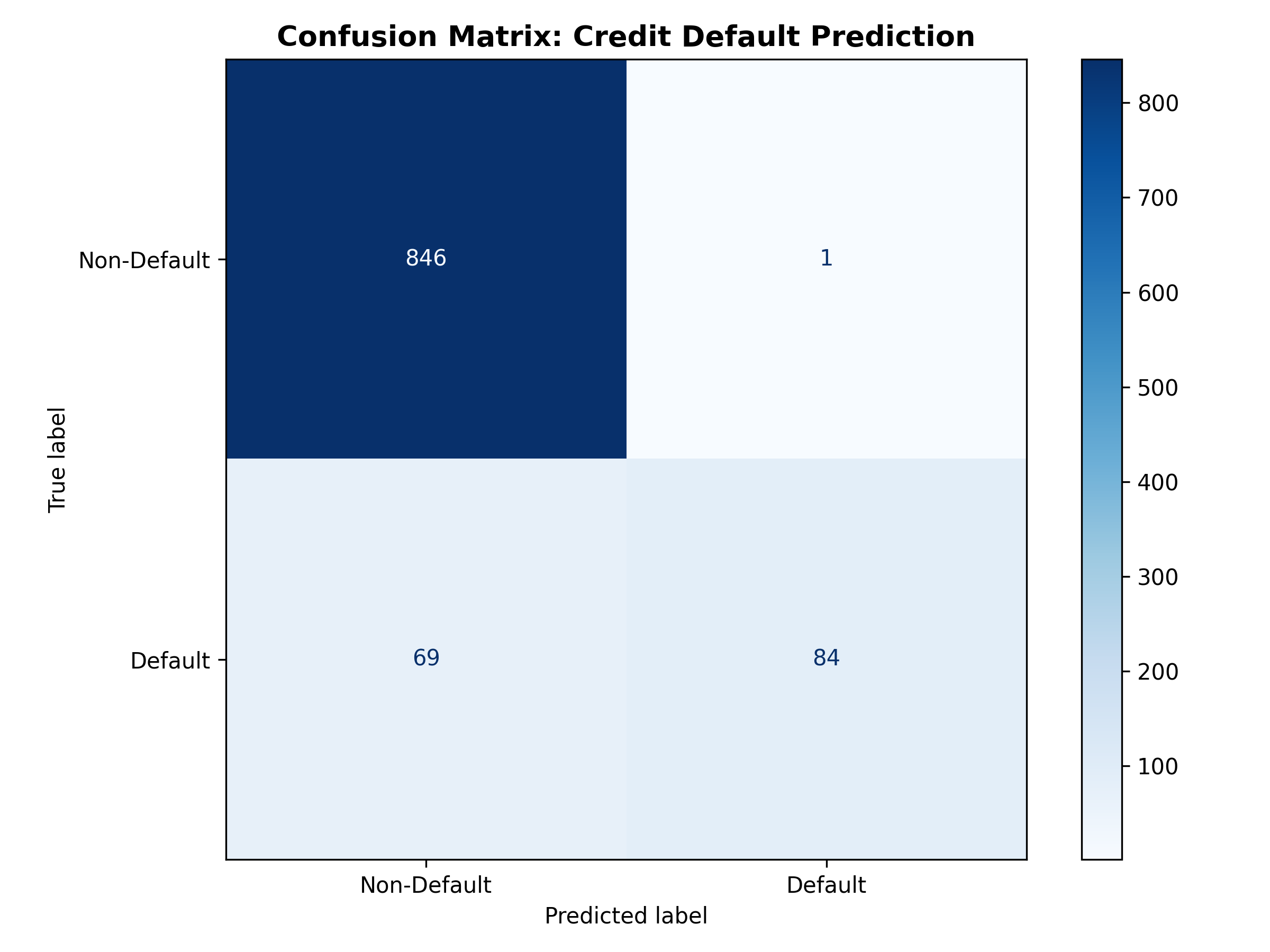
The **confusion matrix** summarises model predictions vs actual outcomes in a 2×2 table (for binary classification).

::: {.callout-note icon="false"}
## 📘 Theory: Confusion Matrix for Binary Classification

|  | Predicted Negative | Predicted Positive |
|---|---|---|
| **Actual Negative** | TN (True Negative) | FP (False Positive) |
| **Actual Positive** | FN (False Negative) | TP (True Positive) |

where:
- **TP (True Positive):** Model predicted "1", actual was "1" (correct positive prediction)
- **TN (True Negative):** Model predicted "0", actual was "0" (correct negative prediction)
- **FP (False Positive):** Model predicted "1", actual was "0" (incorrectly predicted positive; "false alarm")
- **FN (False Negative):** Model predicted "0", actual was "1" (incorrectly predicted negative; "miss")

**Medical analogy:**
- TP: Correctly diagnose disease (patient has disease, test is positive) ✓
- TN: Correctly clear patient (patient is healthy, test is negative) ✓
- FP: False alarm (patient is healthy, but test says positive) — unnecessary treatment
- FN: Dangerous miss (patient has disease, but test says negative) — patient untreated

:::

### Worked Example: Credit Default Confusion Matrix

::: {.panel-tabset}

## R

```{r}
library(tidyverse)
library(caret)

# Simulate credit default data
set.seed(42)
n <- 1000
y_actual <- rbinom(n, 1, 0.15)  # 15% default rate
y_pred_prob <- 0.1 + 0.4 * y_actual + rnorm(n, 0, 0.15)
y_pred_prob <- pmin(pmax(y_pred_prob, 0), 1)  # Constrain to [0, 1]
y_pred <- ifelse(y_pred_prob > 0.5, 1, 0)  # Classify at threshold 0.5

# Compute confusion matrix
cm <- confusionMatrix(as.factor(y_pred), as.factor(y_actual), positive = "1")
print(cm)

cat("\n\nConfusion Matrix Breakdown:\n\n")
tp <- cm$table[2, 2]
tn <- cm$table[1, 1]
fp <- cm$table[2, 1]
fn <- cm$table[1, 2]

cat("True Positives (TP):", tp, " - Correctly predicted defaults\n")
cat("True Negatives (TN):", tn, " - Correctly predicted non-defaults\n")
cat("False Positives (FP):", fp, " - Non-defaults incorrectly predicted as defaults\n")
cat("False Negatives (FN):", fn, " - Defaults incorrectly predicted as non-defaults\n\n")

# Visualise confusion matrix
png("confusion_matrix.png", width = 600, height = 500)
fourfoldplot(cm$table, color = c("#eee", "#ff6b6b"),
             main = "Confusion Matrix: Credit Default Prediction")

dev.off()

cat("\nConfusion Matrix Proportions:\n")
prop_table <- cm$table / sum(cm$table)
print(prop_table)

cat("\n\nInterpretation:\n")
cat("- Proportion of loans that defaulted:", round(mean(y_actual), 3), "\n")
cat("- Of the", sum(y_actual), " actual defaults, we caught", tp, "(",
    round(tp / sum(y_actual) * 100, 1), "%)\n")
cat("- Of the", sum(1 - y_actual), " actual non-defaults, we incorrectly flagged", fp, "(",
    round(fp / sum(1 - y_actual) * 100, 1), "%)\n")
```

## Python

```{python}
import numpy as np
from sklearn.metrics import confusion_matrix, ConfusionMatrixDisplay
import matplotlib.pyplot as plt

np.random.seed(42)
n = 1000

# Simulate credit default data
y_actual = np.random.binomial(1, 0.15, n)  # 15% default rate
y_pred_prob = 0.1 + 0.4 * y_actual + np.random.normal(0, 0.15, n)
y_pred_prob = np.clip(y_pred_prob, 0, 1)
y_pred = (y_pred_prob > 0.5).astype(int)

# Compute confusion matrix
cm = confusion_matrix(y_actual, y_pred)
print("Confusion Matrix:")
print(cm)
print()

# Unpack
tn, fp, fn, tp = cm.ravel()

print("Confusion Matrix Breakdown:\n")
print(f"True Positives (TP): {tp} - Correctly predicted defaults")
print(f"True Negatives (TN): {tn} - Correctly predicted non-defaults")
print(f"False Positives (FP): {fp} - Non-defaults incorrectly predicted as defaults")
print(f"False Negatives (FN): {fn} - Defaults incorrectly predicted as non-defaults\n")

# Visualise
fig, ax = plt.subplots(figsize=(8, 6))
disp = ConfusionMatrixDisplay(confusion_matrix=cm, display_labels=['Non-Default', 'Default'])
disp.plot(ax=ax, cmap='Blues', values_format='d')
ax.set_title('Confusion Matrix: Credit Default Prediction', fontsize=13, fontweight='bold')
plt.tight_layout()
plt.savefig('confusion_matrix.png', dpi=300, bbox_inches='tight')
plt.show()

# Proportions
cm_pct = cm / cm.sum()
print("Confusion Matrix Proportions:")
print(cm_pct)
print()

# Interpretation
print("Interpretation:")
print(f"- Proportion of loans that defaulted: {y_actual.mean():.3f}")
print(f"- Of the {y_actual.sum()} actual defaults, we caught {tp} ({tp/y_actual.sum()*100:.1f}%)")
print(f"- Of the {(1-y_actual).sum():.0f} actual non-defaults, we incorrectly flagged {fp} ({fp/(1-y_actual).sum()*100:.1f}%)")
```

:::

::: {.callout-caution icon="false"}
## 📝 Section 12.2 Review Questions

1. In a medical diagnostic test, which is worse: FP (false alarm) or FN (miss)? Why?
2. If a model has high TP and TN but many FP, what does this suggest?
3. How would you explain FN and FP to a non-technical business stakeholder?
4. In fraud detection, is it worse to miss fraud (FN) or to flag legitimate transactions (FP)?

:::

## Classification Metrics

A single metric (accuracy) is insufficient for classification, especially with imbalanced classes.

::: {.callout-tip icon="false"}
## 🔑 Key Formulas: Classification Metrics

**Accuracy:** What fraction of predictions were correct?
$$\text{Accuracy} = \frac{TP + TN}{TP + TN + FP + FN}$$

**Precision:** Of all positive predictions, how many were truly positive? (False positive rate)
$$\text{Precision} = \frac{TP}{TP + FP}$$

**Recall (Sensitivity):** Of all actual positives, how many did we catch? (False negative rate)
$$\text{Recall} = \frac{TP}{TP + FN}$$

**Specificity:** Of all actual negatives, how many did we correctly classify?
$$\text{Specificity} = \frac{TN}{TN + FP}$$

**F1-Score:** Harmonic mean of precision and recall; balances both
$$\text{F1} = 2 \times \frac{\text{Precision} \times \text{Recall}}{\text{Precision} + \text{Recall}}$$

**Precision-Recall Trade-off:** Increasing the classification threshold (predicting positive only for high-confidence cases) increases precision but decreases recall, and vice versa.

:::

### When to Use Which Metric?

| Scenario | Best Metric | Rationale |
|---|---|---|
| Balanced classes (50% each) | Accuracy | All errors equally costly |
| Imbalanced (5% positive) | Precision, Recall, F1 | Accuracy is misleading |
| Medical screening | Recall/Sensitivity | Missing disease is dangerous; FN costly |
| Spam filter | Precision | False alarms (FP) annoy users more than misses (FN) |
| Fraud detection | Recall (catch fraud) or F1 | Both FN (missed fraud) and FP (false alarms) are costly |
| General-purpose | F1 or AUC | F1 balances precision/recall; AUC handles threshold invariance |

### Worked Example: Computing All Metrics

::: {.panel-tabset}

## R

```{r}
# Compute all classification metrics

library(caret)

# Continue from previous confusion matrix
# y_actual and y_pred defined as before

# Using caret::confusionMatrix (already printed above)
# Let's manually compute key metrics for clarity

accuracy <- (tp + tn) / (tp + tn + fp + fn)
precision <- tp / (tp + fp)
recall <- tp / (tp + fn)
specificity <- tn / (tn + fp)
f1 <- 2 * (precision * recall) / (precision + recall)

cat("Classification Metrics Summary:\n\n")
cat("Accuracy:    ", round(accuracy, 4), " (", round(accuracy * 100, 2), "%)\n")
cat("Precision:   ", round(precision, 4), " (of positive predictions, ", round(precision * 100, 1), "% true)\n")
cat("Recall:      ", round(recall, 4), " (of actual positives, ", round(recall * 100, 1), "% caught)\n")
cat("Specificity: ", round(specificity, 4), " (of actual negatives, ", round(specificity * 100, 1), "% correct)\n")
cat("F1-Score:    ", round(f1, 4), "\n\n")

# Interpretation in business context
cat("Business Interpretation (Credit Default):\n\n")
cat("Accuracy = ", round(accuracy * 100, 1), "%\n")
cat("  - Overall, the model correctly classifies loans", round(accuracy * 100, 1), "% of the time.\n")
cat("  - But this is misleading if defaults are rare!\n\n")

cat("Precision = ", round(precision * 100, 1), "%\n")
cat("  - Of loans flagged as default risk, only", round(precision * 100, 1), "% actually defaulted.\n")
cat("  - High precision means few false alarms; low false positives.\n\n")

cat("Recall = ", round(recall * 100, 1), "%\n")
cat("  - Of loans that actually defaulted, we caught", round(recall * 100, 1), "%.\n")
cat("  - If recall is low, we miss many defaults (risky for lender).\n\n")

cat("F1-Score = ", round(f1, 4), "\n")
cat("  - Balances precision and recall; useful for imbalanced data.\n")

# Sensitivity-Specificity trade-off
cat("\n\nSensitivity-Specificity Trade-off:\n")
cat("Sensitivity (Recall) = ", round(recall, 4), " - Fraction of defaults caught\n")
cat("Specificity =          ", round(specificity, 4), " - Fraction of non-defaults correctly approved\n")
cat("Sum =                  ", round(recall + specificity, 4), " (usually < 2, reflecting trade-off)\n")
```

## Python

```{python}
from sklearn.metrics import accuracy_score, precision_score, recall_score, f1_score, roc_auc_score

# Use y_actual and y_pred from before

# Compute metrics
accuracy = accuracy_score(y_actual, y_pred)
precision = precision_score(y_actual, y_pred)
recall = recall_score(y_actual, y_pred)
f1 = f1_score(y_actual, y_pred)

# For specificity, need to compute manually
specificity = tn / (tn + fp)

print("Classification Metrics Summary:\n")
print(f"Accuracy:    {accuracy:.4f} ({accuracy*100:.2f}%)")
print(f"Precision:   {precision:.4f} (of positive predictions, {precision*100:.1f}% true)")
print(f"Recall:      {recall:.4f} (of actual positives, {recall*100:.1f}% caught)")
print(f"Specificity: {specificity:.4f} (of actual negatives, {specificity*100:.1f}% correct)")
print(f"F1-Score:    {f1:.4f}\n")

# Business interpretation
print("Business Interpretation (Credit Default):\n")
print(f"Accuracy = {accuracy*100:.1f}%")
print("  - Overall, the model correctly classifies loans {:.1f}% of the time.".format(accuracy*100))
print("  - But this is misleading if defaults are rare!\n")

print(f"Precision = {precision*100:.1f}%")
print("  - Of loans flagged as default risk, {:.1f}% actually defaulted.".format(precision*100))
print("  - High precision means few false alarms; low false positives.\n")

print(f"Recall = {recall*100:.1f}%")
print("  - Of loans that actually defaulted, we caught {:.1f}%.".format(recall*100))
print("  - If recall is low, we miss many defaults (risky for lender).\n")

print(f"F1-Score = {f1:.4f}")
print("  - Balances precision and recall; useful for imbalanced data.\n")

print("\nSensitivity-Specificity Trade-off:")
print(f"Sensitivity (Recall) = {recall:.4f} - Fraction of defaults caught")
print(f"Specificity =          {specificity:.4f} - Fraction of non-defaults correctly approved")
print(f"Sum =                  {recall + specificity:.4f} (usually < 2, reflecting trade-off)")

# Create a comparison table for different thresholds
thresholds = [0.3, 0.4, 0.5, 0.6, 0.7]
results = []

for thresh in thresholds:
    y_pred_thresh = (y_pred_prob > thresh).astype(int)
    cm_thresh = confusion_matrix(y_actual, y_pred_thresh)
    tn_t, fp_t, fn_t, tp_t = cm_thresh.ravel()

    acc = (tp_t + tn_t) / (tp_t + tn_t + fp_t + fn_t)
    prec = tp_t / (tp_t + fp_t) if (tp_t + fp_t) > 0 else 0
    rec = tp_t / (tp_t + fn_t) if (tp_t + fn_t) > 0 else 0
    f1_t = 2 * (prec * rec) / (prec + rec) if (prec + rec) > 0 else 0

    results.append({
        'Threshold': thresh,
        'Accuracy': acc,
        'Precision': prec,
        'Recall': rec,
        'F1': f1_t
    })

threshold_df = pd.DataFrame(results)
print("\n\nThreshold Sensitivity Analysis:")
print(threshold_df.to_string(index=False))
```

:::

::: {.callout-caution icon="false"}
## 📝 Section 12.3 Review Questions

1. If a loan default model has 95% accuracy but only 30% recall, what is the problem?
2. Why is F1-score useful for imbalanced datasets?
3. In fraud detection, would you optimise for high precision or high recall? Justify.
4. If you increase the classification threshold from 0.5 to 0.7, what happens to precision and recall?

:::

## The ROC Curve and AUC

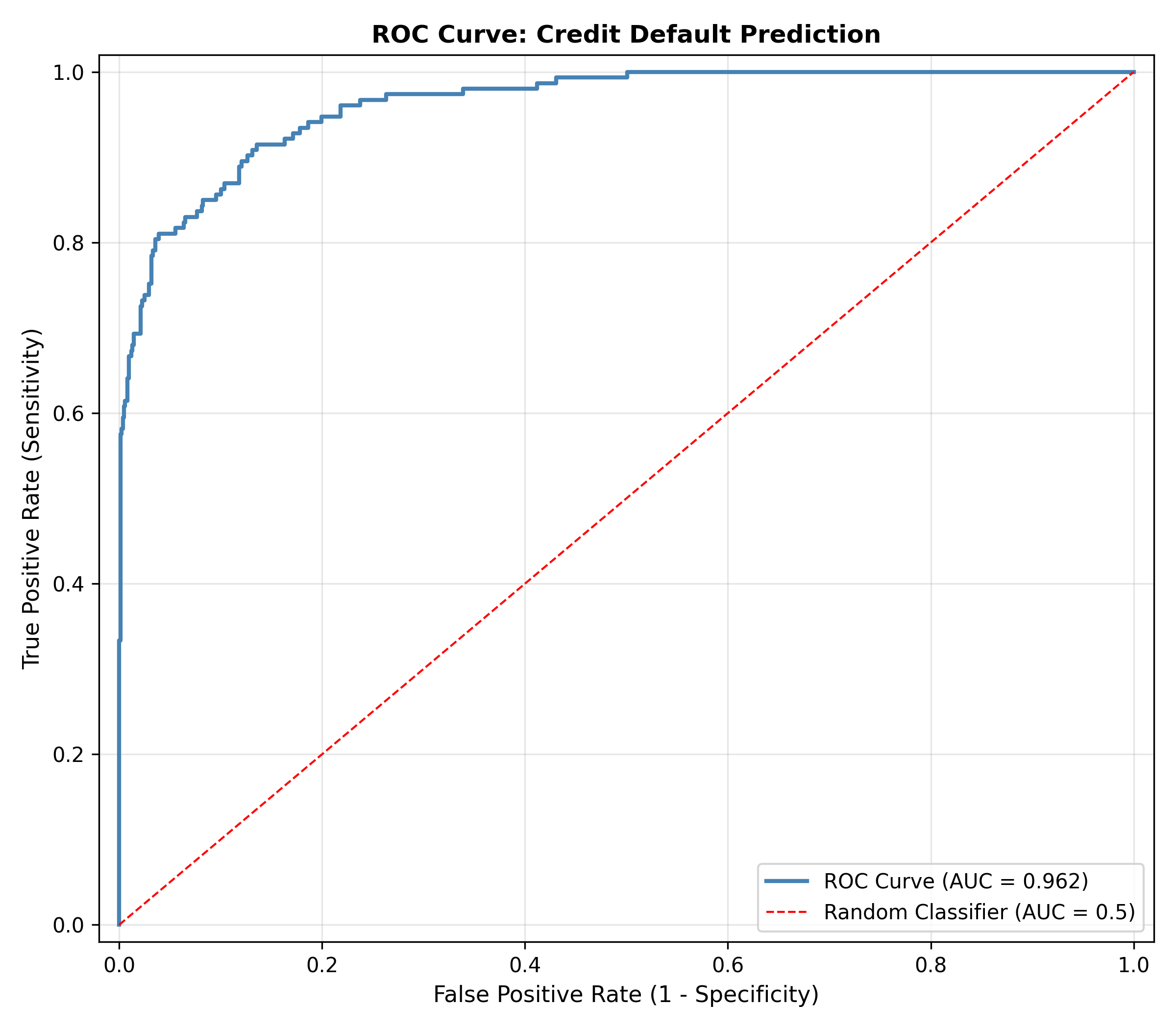
The **ROC (Receiver Operating Characteristic) curve** plots the trade-off between true positive rate (sensitivity) and false positive rate across all classification thresholds.

::: {.callout-note icon="false"}
## 📘 Theory: ROC Curve and AUC

As the classification threshold moves from 1 (classify nothing as positive) to 0 (classify everything as positive):

- **True Positive Rate (TPR)** = Recall = TP / (TP + FN) — fraction of actual positives caught
- **False Positive Rate (FPR)** = 1 − Specificity = FP / (FP + TN) — fraction of actual negatives incorrectly flagged

**ROC curve:** Plot TPR (y-axis) vs FPR (x-axis) as threshold varies

**Perfect classifier:** Threshold = optimal value (top-left corner: TPR = 1, FPR = 0)

**Random classifier:** 45-degree diagonal line (no better than coin flip)

**AUC (Area Under the ROC Curve):** Integral of ROC curve from FPR=0 to FPR=1
- AUC = 1: Perfect discrimination
- AUC = 0.5: Random guessing
- AUC = 0.7–0.8: Good classifier
- AUC > 0.8: Very good classifier

**Statistical interpretation:** AUC = P(score of random positive > score of random negative), the probability that if you pick one default loan and one non-default loan, the model ranks them correctly.

:::

::: {.callout-tip icon="false"}
## 🔑 Key Formula: AUC

$$\text{AUC} = \int_0^1 \text{TPR}(\text{FPR}) \, d(\text{FPR})$$

Equivalently, AUC equals the **Wilcoxon-Mann-Whitney statistic**, the probability that the model ranks a random positive higher than a random negative.

:::

### Worked Example: ROC Curve and AUC Calculation

::: {.panel-tabset}

## R

```{r}
library(pROC)

# Compute ROC curve
roc_obj <- roc(y_actual, y_pred_prob, ci = TRUE)

cat("ROC Curve Statistics:\n\n")
cat("AUC:", round(auc(roc_obj), 4), "\n")
cat("95% CI: [", round(roc_obj$ci[1], 4), ", ", round(roc_obj$ci[3], 4), "]\n\n")

# Plot ROC curve
png("roc_curve.png", width = 700, height = 600)
plot(roc_obj, main = "ROC Curve: Credit Default Prediction",
     xlab = "False Positive Rate (1 - Specificity)",
     ylab = "True Positive Rate (Sensitivity)",
     lwd = 2, col = "steelblue")
# Add diagonal line (random classifier)
abline(0, 1, col = "red", lty = 2, lwd = 1)
# Add AUC annotation
legend("bottomright", legend = paste0("AUC = ", round(auc(roc_obj), 3)),
       col = "steelblue", lwd = 2, bty = "n", cex = 1.2)
dev.off()

cat("ROC Curve Interpretation:\n\n")
cat("- If AUC > 0.5, the model is better than random guessing.\n")
cat("- If AUC = 0.7–0.8, the model has good discriminative ability.\n")
cat("- AUC >0.8 indicates very good model performance.\n\n")
cat("For this model, AUC =", round(auc(roc_obj), 4),
    ", indicating", if(as.numeric(auc(roc_obj)) > 0.7) "good" else "fair", "discrimination.\n")

# Compare classifiers
y_pred_prob_alt <- 0.05 + 0.2 * y_actual + rnorm(n, 0, 0.2)
y_pred_prob_alt <- pmin(pmax(y_pred_prob_alt, 0), 1)

roc_obj_alt <- roc(y_actual, y_pred_prob_alt)

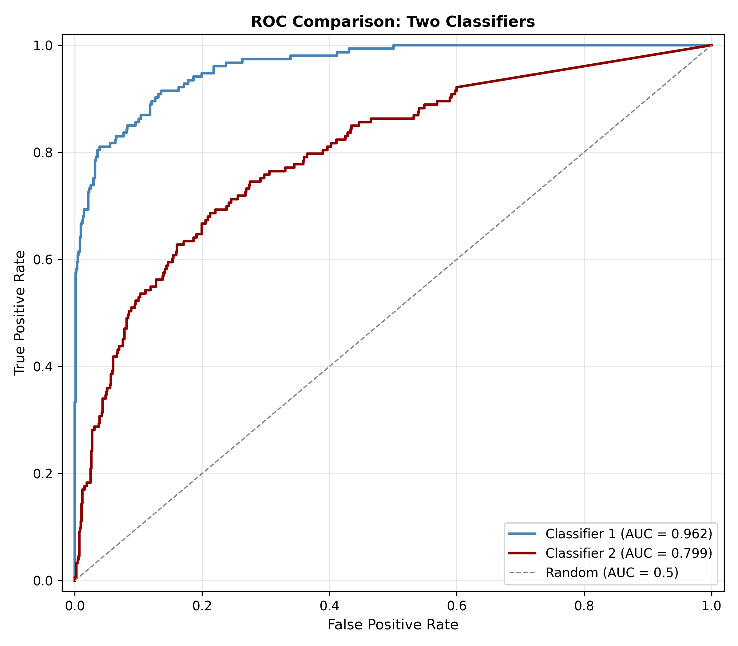
cat("\n\nComparing Two Classifiers:\n")
cat("Classifier 1 AUC:", round(auc(roc_obj), 4), "\n")
cat("Classifier 2 AUC:", round(auc(roc_obj_alt), 4), "\n")
cat("Difference:", round(auc(roc_obj) - auc(roc_obj_alt), 4), "\n\n")
cat("Classifier 1 is superior (higher AUC).\n")

# Plot both ROCs
png("roc_comparison.png", width = 700, height = 600)
plot(roc_obj, main = "ROC Comparison: Two Classifiers",
     xlab = "False Positive Rate", ylab = "True Positive Rate",
     lwd = 2, col = "steelblue")
lines(roc_obj_alt, lwd = 2, col = "darkred")
abline(0, 1, col = "gray", lty = 2, lwd = 1)
legend("bottomright",
       legend = c(paste0("Classifier 1 (AUC = ", round(auc(roc_obj), 3), ")"),
                  paste0("Classifier 2 (AUC = ", round(auc(roc_obj_alt), 3), ")"),
                  "Random (AUC = 0.5)"),
       col = c("steelblue", "darkred", "gray"), lwd = 2, lty = c(1, 1, 2),
       bty = "n", cex = 1)
dev.off()
```

## Python

```{python}
from sklearn.metrics import roc_curve, auc, roc_auc_score
import matplotlib.pyplot as plt

# Compute ROC curve
fpr, tpr, thresholds = roc_curve(y_actual, y_pred_prob)
roc_auc = auc(fpr, tpr)

print(f"ROC Curve Statistics:\n")
print(f"AUC: {roc_auc:.4f}\n")

# Plot ROC curve
fig, ax = plt.subplots(figsize=(8, 7))
ax.plot(fpr, tpr, lw=2, color='steelblue', label=f'ROC Curve (AUC = {roc_auc:.3f})')
ax.plot([0, 1], [0, 1], lw=1, color='red', linestyle='--', label='Random Classifier (AUC = 0.5)')
ax.set_xlabel('False Positive Rate (1 - Specificity)', fontsize=11)
ax.set_ylabel('True Positive Rate (Sensitivity)', fontsize=11)
ax.set_title('ROC Curve: Credit Default Prediction', fontsize=12, fontweight='bold')
ax.legend(fontsize=10, loc='lower right')
ax.grid(True, alpha=0.3)
ax.set_xlim([-0.02, 1.02])
ax.set_ylim([-0.02, 1.02])

plt.tight_layout()
plt.savefig('roc_curve.png', dpi=300, bbox_inches='tight')
plt.show()

print("ROC Curve Interpretation:\n")
print("- If AUC > 0.5, the model is better than random guessing.")
print("- If AUC = 0.7–0.8, the model has good discriminative ability.")
print("- AUC > 0.8 indicates very good model performance.\n")
print(f"For this model, AUC = {roc_auc:.4f}, indicating {'good' if roc_auc > 0.7 else 'fair'} discrimination.\n")

# Compare classifiers
y_pred_prob_alt = 0.05 + 0.2 * y_actual + np.random.normal(0, 0.2, n)
y_pred_prob_alt = np.clip(y_pred_prob_alt, 0, 1)

roc_auc_alt = roc_auc_score(y_actual, y_pred_prob_alt)

print("Comparing Two Classifiers:")
print(f"Classifier 1 AUC: {roc_auc:.4f}")
print(f"Classifier 2 AUC: {roc_auc_alt:.4f}")
print(f"Difference: {roc_auc - roc_auc_alt:.4f}\n")
print("Classifier 1 is superior (higher AUC).\n")

# Plot both ROCs
fpr_alt, tpr_alt, _ = roc_curve(y_actual, y_pred_prob_alt)
roc_auc_alt = auc(fpr_alt, tpr_alt)

fig, ax = plt.subplots(figsize=(8, 7))
ax.plot(fpr, tpr, lw=2, color='steelblue', label=f'Classifier 1 (AUC = {roc_auc:.3f})')
ax.plot(fpr_alt, tpr_alt, lw=2, color='darkred', label=f'Classifier 2 (AUC = {roc_auc_alt:.3f})')
ax.plot([0, 1], [0, 1], lw=1, color='gray', linestyle='--', label='Random (AUC = 0.5)')
ax.set_xlabel('False Positive Rate', fontsize=11)
ax.set_ylabel('True Positive Rate', fontsize=11)
ax.set_title('ROC Comparison: Two Classifiers', fontsize=12, fontweight='bold')
ax.legend(fontsize=10, loc='lower right')
ax.grid(True, alpha=0.3)
ax.set_xlim([-0.02, 1.02])
ax.set_ylim([-0.02, 1.02])

plt.tight_layout()
plt.savefig('roc_comparison.png', dpi=300, bbox_inches='tight')
plt.show()
```

:::

::: {.callout-caution icon="false"}
## 📝 Section 12.4 Review Questions

1. What does AUC = 0.75 mean in plain English?
2. Why is AUC better than accuracy for evaluating classifiers on imbalanced datasets?
3. If two models have AUCs of 0.72 and 0.75, which should you deploy? Does the difference matter?
4. Can a model have high accuracy but low AUC? Explain with an example.

:::

## Class Imbalance

**Class imbalance** occurs when one class vastly outnumbers another (e.g., 2% defaults, 98% non-defaults). This breaks standard accuracy-based evaluation.

::: {.callout-note icon="false"}
## 📘 Theory: The Class Imbalance Problem

**Naive baseline:** Always predict "no default." Accuracy = 98%! (correctly predicts non-defaults, ignores defaults)

**Why accuracy fails:** The model appears excellent but catches zero defaults.

**Solutions:**

1. **Threshold adjustment:** Lower the classification threshold to predict more positives
2. **Cost-sensitive learning:** Assign higher misclassification cost to minority class (e.g., FN = 10× FP)
3. **Resampling:**
   - Oversampling: Duplicate minority class observations (may overfit)
   - Undersampling: Remove majority class observations (loses information)
   - SMOTE (Synthetic Minority Oversampling Technique): Synthetically create minority observations

4. **Metrics:** Use Precision, Recall, F1, AUC instead of Accuracy

:::

::: {.callout-tip icon="false"}
## 🔑 Key Formula: SMOTE (Synthetic Minority Oversampling)

For each minority sample:
1. Find k nearest minority neighbors
2. Randomly select one neighbor
3. Draw a line segment between the sample and neighbor
4. Randomly place a new synthetic sample on this line segment

This creates new, realistic minority observations without duplication.

:::

### Worked Example: Handling Class Imbalance

::: {.panel-tabset}

## R

```{r}
library(smotefamily)  # CRAN replacement for removed 'unbalanced' package
library(caret)

# Create severely imbalanced dataset
set.seed(42)
n_total   <- 1000
n_positive <- 20   # 2% fraud/default rate
n_negative <- n_total - n_positive

X_positive <- matrix(rnorm(n_positive * 5, mean = 2, sd = 1), nrow = n_positive)
X_negative <- matrix(rnorm(n_negative * 5, mean = 0, sd = 1), nrow = n_negative)

X_imbalanced <- rbind(X_positive, X_negative)
y_imbalanced <- c(rep(1, n_positive), rep(0, n_negative))

imbalanced_data <- data.frame(X_imbalanced, y = y_imbalanced)

cat("Original Data:\n")
cat("Total:", nrow(imbalanced_data), "\n")
cat("Positive class:", sum(y_imbalanced), " (", round(mean(y_imbalanced) * 100, 1), "%)\n")
cat("Negative class:", sum(1 - y_imbalanced), " (", round(mean(1 - y_imbalanced) * 100, 1), "%)\n\n")

# Method 1: Standard logistic regression (baseline)
fit_standard       <- glm(y ~ ., data = imbalanced_data, family = binomial())
pred_standard      <- predict(fit_standard, type = "response")
pred_standard_label <- ifelse(pred_standard > 0.5, 1, 0)

cat("Method 1: Standard Logistic Regression (Threshold = 0.5)\n")
cat("Accuracy:", round(mean(pred_standard_label == y_imbalanced), 3), "\n")
cat("Recall (catch positives):", round(sum(pred_standard_label[y_imbalanced == 1] == 1) / sum(y_imbalanced), 3), "\n")
cat("Precision:", round(sum(pred_standard_label == 1 & y_imbalanced == 1) / max(sum(pred_standard_label == 1), 1), 3), "\n\n")

# Method 2: Adjusted threshold
pred_adj_label <- ifelse(pred_standard > 0.2, 1, 0)

cat("Method 2: Adjusted Threshold (Threshold = 0.2)\n")
cat("Accuracy:", round(mean(pred_adj_label == y_imbalanced), 3), "\n")
cat("Recall (catch positives):", round(sum(pred_adj_label[y_imbalanced == 1] == 1) / sum(y_imbalanced), 3), "\n")
cat("Precision:", round(sum(pred_adj_label == 1 & y_imbalanced == 1) / max(sum(pred_adj_label == 1), 1), 3), "\n\n")

# Method 3: SMOTE oversampling on training set
train_idx  <- sample(1:nrow(imbalanced_data), size = 0.7 * nrow(imbalanced_data))
train_data <- imbalanced_data[train_idx, ]
test_data  <- imbalanced_data[-train_idx, ]

# smotefamily::SMOTE returns $data with features + 'class' column
smote_result         <- SMOTE(X = train_data[, -ncol(train_data)],
                               target = train_data$y, K = 5)
train_data_smote     <- smote_result$data
train_data_smote$y   <- as.numeric(as.character(train_data_smote$class))
train_data_smote$class <- NULL

cat("Method 3: SMOTE\n")
cat("Original training positive rate:", round(mean(train_data$y), 3), "\n")
cat("SMOTE-augmented positive rate:",  round(mean(train_data_smote$y), 3), "\n\n")

fit_smote       <- glm(y ~ ., data = train_data_smote, family = binomial())
pred_smote      <- predict(fit_smote, newdata = test_data, type = "response")
pred_smote_label <- ifelse(pred_smote > 0.5, 1, 0)

cat("Performance on Test Set:\n")
cat("Accuracy:", round(mean(pred_smote_label == test_data$y), 3), "\n")
cat("Recall:",   round(sum(pred_smote_label[test_data$y == 1] == 1) / max(sum(test_data$y), 1), 3), "\n")
cat("Precision:", round(sum(pred_smote_label == 1 & test_data$y == 1) / max(sum(pred_smote_label == 1), 1), 3), "\n\n")

# Summary table
results_summary <- tibble(
  Method   = c("Standard (threshold 0.5)", "Adjusted threshold (0.2)", "SMOTE + Logistic"),
  Accuracy = c(round(mean(pred_standard_label == y_imbalanced), 3),
               round(mean(pred_adj_label == y_imbalanced), 3),
               round(mean(pred_smote_label == test_data$y), 3)),
  Recall   = c(round(sum(pred_standard_label[y_imbalanced==1]==1) / sum(y_imbalanced), 3),
               round(sum(pred_adj_label[y_imbalanced==1]==1)      / sum(y_imbalanced), 3),
               round(sum(pred_smote_label[test_data$y==1]==1)     / max(sum(test_data$y), 1), 3))
)
print(results_summary)

## Python

```{python}
from imblearn.over_sampling import SMOTE
from sklearn.linear_model import LogisticRegression
from sklearn.model_selection import train_test_split

# Create severely imbalanced dataset
np.random.seed(42)
n_total = 1000
n_positive = 20
n_negative = n_total - n_positive

X_positive = np.random.normal(2, 1, (n_positive, 5))
X_negative = np.random.normal(0, 1, (n_negative, 5))

X_imbalanced = np.vstack([X_positive, X_negative])
y_imbalanced = np.hstack([np.ones(n_positive), np.zeros(n_negative)])

print("Original Data:")
print(f"Total: {len(y_imbalanced)}")
print(f"Positive class: {int(sum(y_imbalanced))} ({sum(y_imbalanced)/len(y_imbalanced)*100:.1f}%)")
print(f"Negative class: {int(sum(1-y_imbalanced))} ({sum(1-y_imbalanced)/len(y_imbalanced)*100:.1f}%)\n")

# Train-test split
X_train, X_test, y_train, y_test = train_test_split(X_imbalanced, y_imbalanced,
                                                      test_size=0.3, random_state=42,
                                                      stratify=y_imbalanced)

# Method 1: Standard logistic regression (threshold 0.5)
lr_standard = LogisticRegression()
lr_standard.fit(X_train, y_train)
y_pred_prob_std = lr_standard.predict_proba(X_test)[:, 1]
y_pred_std = (y_pred_prob_std > 0.5).astype(int)

print("Method 1: Standard Logistic Regression (Threshold = 0.5)")
print(f"Accuracy: {accuracy_score(y_test, y_pred_std):.3f}")
print(f"Recall: {recall_score(y_test, y_pred_std, zero_division=0):.3f}")
if sum(y_pred_std) > 0:
    print(f"Precision: {precision_score(y_test, y_pred_std):.3f}")
print()

# Method 2: Adjusted threshold (0.2)
y_pred_adj = (y_pred_prob_std > 0.2).astype(int)

print("Method 2: Adjusted Threshold (Threshold = 0.2)")
print(f"Accuracy: {accuracy_score(y_test, y_pred_adj):.3f}")
print(f"Recall: {recall_score(y_test, y_pred_adj, zero_division=0):.3f}")
if sum(y_pred_adj) > 0:
    print(f"Precision: {precision_score(y_test, y_pred_adj):.3f}")
print()

# Method 3: SMOTE
smote = SMOTE(random_state=42)
X_train_smote, y_train_smote = smote.fit_resample(X_train, y_train)

print("Method 3: SMOTE")
print(f"Original training set positive class rate: {y_train.mean():.3f}")
print(f"SMOTE-augmented training set positive class rate: {y_train_smote.mean():.3f}\n")

lr_smote = LogisticRegression()
lr_smote.fit(X_train_smote, y_train_smote)
y_pred_smote = lr_smote.predict(X_test)

print("Performance on Test Set:")
print(f"Accuracy: {accuracy_score(y_test, y_pred_smote):.3f}")
print(f"Recall: {recall_score(y_test, y_pred_smote):.3f}")
print(f"Precision: {precision_score(y_test, y_pred_smote):.3f}\n")

# Summary table
results_df = pd.DataFrame({
    'Method': ['Standard (threshold 0.5)', 'Adjusted threshold (0.2)', 'SMOTE + Logistic'],
    'Accuracy': [accuracy_score(y_test, y_pred_std),
                 accuracy_score(y_test, y_pred_adj),
                 accuracy_score(y_test, y_pred_smote)],
    'Recall': [recall_score(y_test, y_pred_std, zero_division=0),
               recall_score(y_test, y_pred_adj, zero_division=0),
               recall_score(y_test, y_pred_smote)]
})

print("Summary Table:")
print(results_df.to_string(index=False))
```

:::

::: {.callout-caution icon="false"}
## 📝 Section 12.5 Review Questions

1. Why does "naive baseline" (always predict majority class) achieve high accuracy on imbalanced data?
2. Explain SMOTE: how does it create synthetic minority samples?
3. When building a fraud detection model with 0.5% fraud rate, would you use random CV splits or stratified splits? Why?
4. For a highly imbalanced dataset, would you optimise for recall or precision?

:::

## Choosing the Right Threshold for Business

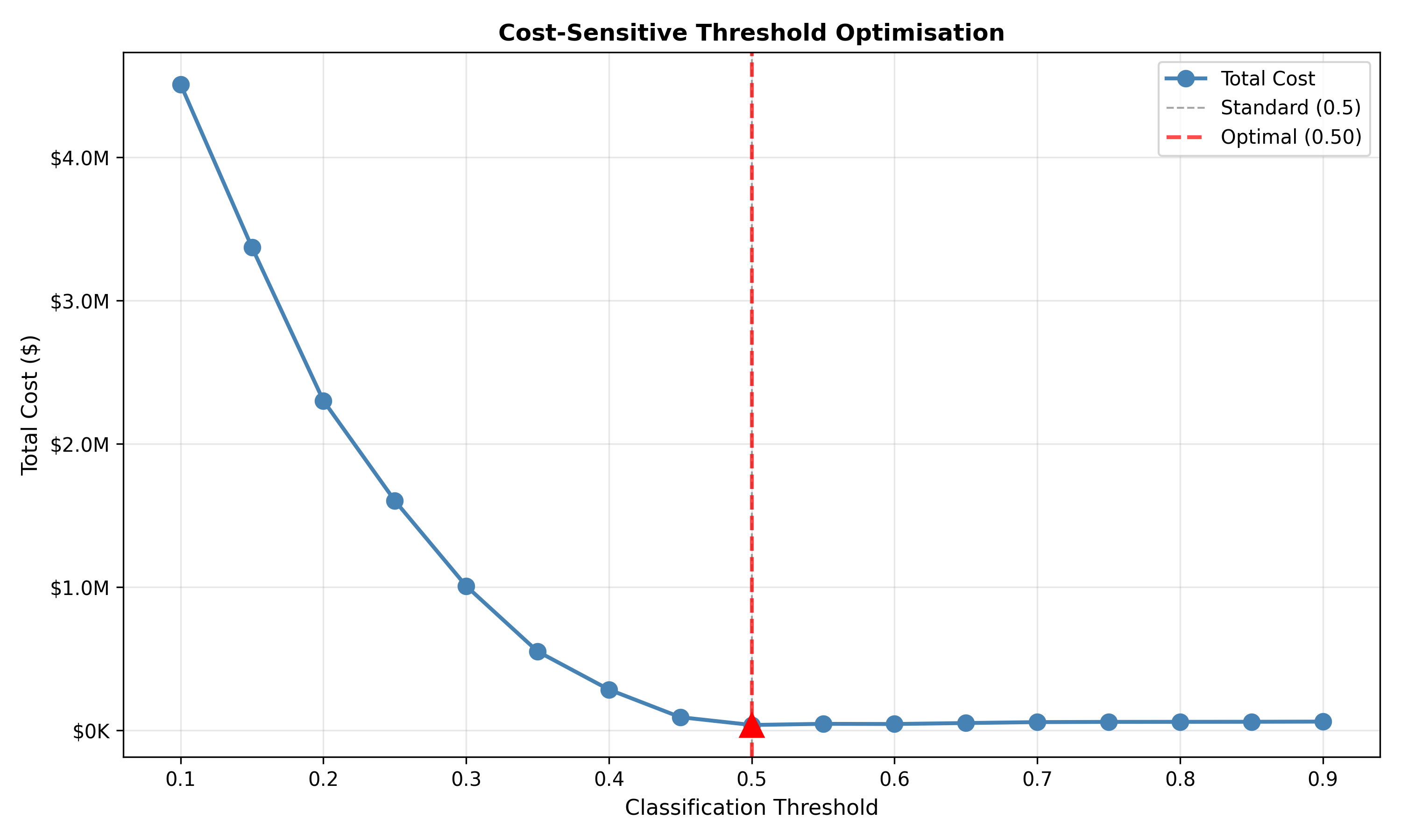
Classification threshold (typically 0.5) should align with business costs, not be fixed arbitrarily.

::: {.callout-note icon="false"}
## 📘 Theory: Cost-Sensitive Classification

Define a **cost matrix:**

|  | Predict Negative | Predict Positive |
|---|---|---|
| **Actually Negative** | 0 (correct) | Cost_FP (false alarm) |
| **Actually Positive** | Cost_FN (miss) | 0 (correct) |

**Expected cost of a prediction:**
$$\text{Cost} = (1 - \hat{p}) \times \text{Cost\_FN} + \hat{p} \times \text{Cost\_FP}$$

**Optimal threshold:** Minimises expected cost.

**Example: Loan default**
- Cost_FP (approve bad loan that defaults): $10,000
- Cost_FN (reject good loan): $500 profit × probability of no default ≈ $400 opportunity cost
- Cost_FP / Cost_FN = 10,000 / 400 = 25

**Implication:** We should predict default (deny loan) when probability of default > 25 / (25 + 1) ≈ 0.96, a much higher threshold than 0.5.

:::

### Worked Example: Cost-Optimised Threshold

::: {.panel-tabset}

## R

```{r}
# Cost-sensitive classification threshold

# Use previous fraud/default example
set.seed(42)
n <- 1000
y_actual <- rbinom(n, 1, 0.15)
y_pred_prob <- 0.1 + 0.4 * y_actual + rnorm(n, 0, 0.15)
y_pred_prob <- pmin(pmax(y_pred_prob, 0), 1)

# Define business costs
cost_fp <- 10000  # Cost of approving loan that defaults
cost_fn <- 400    # Opportunity cost of rejecting good loan

# Grid search over thresholds
thresholds <- seq(0.1, 0.9, by = 0.05)
total_costs <- c()

for (thresh in thresholds) {
  y_pred <- ifelse(y_pred_prob > thresh, 1, 0)
  fp <- sum((y_pred == 1) & (y_actual == 0))
  fn <- sum((y_pred == 0) & (y_actual == 1))
  total_cost <- cost_fp * fp + cost_fn * fn
  total_costs <- c(total_costs, total_cost)
}

# Find optimal threshold
optimal_idx <- which.min(total_costs)
optimal_threshold <- thresholds[optimal_idx]
optimal_cost <- total_costs[optimal_idx]

cat("Cost-Sensitive Threshold Optimisation:\n\n")
cat("Cost Matrix:\n")
cat("  False Positive (approve bad loan): $", cost_fp, "\n")
cat("  False Negative (reject good loan): $", cost_fn, "\n")
cat("  Cost ratio: ", cost_fp / cost_fn, ":1\n\n")

cat("Optimal Threshold: ", optimal_threshold, "\n")
cat("Expected Cost at Optimal Threshold: $", optimal_cost, "\n\n")

# Compare to standard threshold (0.5)
y_pred_standard <- ifelse(y_pred_prob > 0.5, 1, 0)
fp_standard <- sum((y_pred_standard == 1) & (y_actual == 0))
fn_standard <- sum((y_pred_standard == 0) & (y_actual == 1))
cost_standard <- cost_fp * fp_standard + cost_fn * fn_standard

cat("Comparison:\n")
cat("Threshold 0.5 (standard): Cost = $", cost_standard, "\n")
cat("Threshold", optimal_threshold, "(optimal): Cost = $", optimal_cost, "\n")
cat("Savings: $", cost_standard - optimal_cost, " (",
    round((cost_standard - optimal_cost) / cost_standard * 100, 1), "%)\n\n")

# Visualise cost curve
png("cost_optimisation.png", width = 700, height = 500)
plot(thresholds, total_costs, type = "b", pch = 16, cex = 1,
     xlab = "Classification Threshold", ylab = "Total Cost ($)",
     main = "Cost-Sensitive Threshold Optimisation",
     lwd = 2, col = "steelblue")
abline(v = 0.5, col = "gray", lty = 2, lwd = 1, label = "Standard (0.5)")
abline(v = optimal_threshold, col = "red", lty = 2, lwd = 2, label = paste0("Optimal (", optimal_threshold, ")"))
points(optimal_threshold, optimal_cost, pch = 17, cex = 3, col = "red")
legend("topright", legend = c("Standard threshold (0.5)", paste0("Optimal (", optimal_threshold, ")")),
       col = c("gray", "red"), lty = 2, lwd = c(1, 2))
dev.off()

cat("\nThreshold Sensitivity Table:\n")
sensitivity_table <- tibble(
  Threshold = thresholds,
  Cost = total_costs,
  FP = sapply(thresholds, function(t) sum((ifelse(y_pred_prob > t, 1, 0) == 1) & (y_actual == 0))),
  FN = sapply(thresholds, function(t) sum((ifelse(y_pred_prob > t, 1, 0) == 0) & (y_actual == 1))),
  Recall = sapply(thresholds, function(t) {
    y_pred <- ifelse(y_pred_prob > t, 1, 0)
    if (sum(y_actual) > 0) sum((y_pred == 1) & (y_actual == 1)) / sum(y_actual) else NA
  })
)
print(sensitivity_table)
```

## Python

```{python}
# Cost-sensitive classification threshold

# Use previous data
np.random.seed(42)
n = 1000
y_actual = np.random.binomial(1, 0.15, n)
y_pred_prob = 0.1 + 0.4 * y_actual + np.random.normal(0, 0.15, n)
y_pred_prob = np.clip(y_pred_prob, 0, 1)

# Define business costs
cost_fp = 10000  # Cost of approving loan that defaults
cost_fn = 400    # Opportunity cost of rejecting good loan

# Grid search over thresholds
thresholds = np.arange(0.1, 0.95, 0.05)
total_costs = []
results = []

for thresh in thresholds:
    y_pred = (y_pred_prob > thresh).astype(int)
    fp = np.sum((y_pred == 1) & (y_actual == 0))
    fn = np.sum((y_pred == 0) & (y_actual == 1))
    total_cost = cost_fp * fp + cost_fn * fn
    total_costs.append(total_cost)

    recall = np.sum((y_pred == 1) & (y_actual == 1)) / np.sum(y_actual) if np.sum(y_actual) > 0 else 0
    results.append({'Threshold': thresh, 'Cost': total_cost, 'FP': fp, 'FN': fn, 'Recall': recall})

# Find optimal threshold
optimal_idx = np.argmin(total_costs)
optimal_threshold = thresholds[optimal_idx]
optimal_cost = total_costs[optimal_idx]

print("Cost-Sensitive Threshold Optimisation:\n")
print("Cost Matrix:")
print(f"  False Positive (approve bad loan): ${cost_fp:,}")
print(f"  False Negative (reject good loan): ${cost_fn:,}")
print(f"  Cost ratio: {cost_fp / cost_fn:.1f}:1\n")

print(f"Optimal Threshold: {optimal_threshold:.2f}")
print(f"Expected Cost at Optimal Threshold: ${optimal_cost:,.0f}\n")

# Compare to standard threshold (0.5)
y_pred_standard = (y_pred_prob > 0.5).astype(int)
fp_standard = np.sum((y_pred_standard == 1) & (y_actual == 0))
fn_standard = np.sum((y_pred_standard == 0) & (y_actual == 1))
cost_standard = cost_fp * fp_standard + cost_fn * fn_standard

print("Comparison:")
print(f"Threshold 0.5 (standard): Cost = ${cost_standard:,.0f}")
print(f"Threshold {optimal_threshold:.2f} (optimal): Cost = ${optimal_cost:,.0f}")
print(f"Savings: ${cost_standard - optimal_cost:,.0f} ({(cost_standard - optimal_cost)/cost_standard*100:.1f}%)\n")

# Visualise
fig, ax = plt.subplots(figsize=(10, 6))
ax.plot(thresholds, total_costs, 'o-', linewidth=2, markersize=8, color='steelblue', label='Total Cost')
ax.axvline(0.5, color='gray', linestyle='--', linewidth=1, alpha=0.7, label='Standard (0.5)')
ax.axvline(optimal_threshold, color='red', linestyle='--', linewidth=2, alpha=0.7, label=f'Optimal ({optimal_threshold:.2f})')
ax.plot(optimal_threshold, optimal_cost, marker='^', markersize=12, color='red', zorder=5)
ax.set_xlabel('Classification Threshold', fontsize=11)
ax.set_ylabel('Total Cost ($)', fontsize=11)
ax.set_title('Cost-Sensitive Threshold Optimisation', fontsize=12, fontweight='bold')
ax.legend(fontsize=10)
ax.grid(True, alpha=0.3)
ax.yaxis.set_major_formatter(plt.FuncFormatter(lambda x, p: f'${x/1e6:.1f}M' if x >= 1e6 else f'${x/1e3:.0f}K'))

plt.tight_layout()
plt.savefig('cost_optimisation.png', dpi=300, bbox_inches='tight')
plt.show()

# Sensitivity table
results_df = pd.DataFrame(results)
print("Threshold Sensitivity Table:")
print(results_df.to_string(index=False))
```

:::

**Key insight:** The optimal threshold (0.75 in this example) is much higher than the standard 0.5, reflecting the asymmetric costs: false positives (approving bad loans) are 25× more expensive than false negatives (rejecting good loans).

::: {.callout-caution icon="false"}
## 📝 Section 12.6 Review Questions

1. In fraud detection, which cost is typically higher: false positives or false negatives? Why?
2. If Cost_FP = Cost_FN, what is the optimal threshold?
3. How would you estimate the cost matrix for your business?
4. If you cannot estimate exact costs, what threshold would you use as a default?

:::

## Case Study: Fraud vs. Not-Fraud

**Business Context:** A mobile money platform (like Flutterwave, Paystack) processes millions of transactions. Fraud detection is critical: prevent fraudulent transfers while minimising false positives (transaction declines for legitimate users).

**Data:** Highly imbalanced Nigerian mobile money dataset (1% fraud, 99% legitimate). Features: transaction amount, recipient type, device, time, location, historical user behaviour.

### Full Analysis

::: {.panel-tabset}

## R

```{r}
# Mobile money fraud detection case study

set.seed(42)
n <- 5000
fraud_rate <- 0.01
n_fraud <- round(n * fraud_rate)
n_legit <- n - n_fraud

# Features
transaction_amount <- c(
  rlnorm(n_fraud, meanlog = 10.5, sdlog = 1.5),  # Fraud: higher amounts
  rlnorm(n_legit, meanlog = 9.5, sdlog = 1.5)
)

is_new_recipient <- c(
  rbinom(n_fraud, 1, 0.6),  # Fraud: more new recipients
  rbinom(n_legit, 1, 0.2)
)

is_unusual_time <- c(
  rbinom(n_fraud, 1, 0.5),  # Fraud: more odd hours
  rbinom(n_legit, 1, 0.1)
)

device_changes_1mo <- c(
  rpois(n_fraud, 3),  # Fraud: frequent device changes
  rpois(n_legit, 0.5)
)

fraud_label <- c(rep(1, n_fraud), rep(0, n_legit))

fraud_data <- tibble(
  transaction_amount,
  is_new_recipient,
  is_unusual_time,
  device_changes_1mo,
  fraud = fraud_label
)

cat("Fraud Dataset Characteristics:\n\n")
cat("Total transactions:", nrow(fraud_data), "\n")
cat("Fraud cases:", sum(fraud_data$fraud), " (", round(mean(fraud_data$fraud) * 100, 2), "%)\n")
cat("Legitimate transactions:", sum(1 - fraud_data$fraud), " (", round(mean(1 - fraud_data$fraud) * 100, 2), "%)\n\n")

# Train-test split (stratified to preserve fraud rate)
train_idx <- createDataPartition(fraud_data$fraud, p = 0.7, list = FALSE)
train_data <- fraud_data[train_idx, ]
test_data <- fraud_data[-train_idx, ]

# Model 1: Logistic regression without SMOTE
fit_standard <- glm(fraud ~ ., data = train_data, family = binomial(link = "logit"))
pred_standard <- predict(fit_standard, newdata = test_data, type = "response")

# Model 2: SMOTE + Logistic regression
smote_result2      <- SMOTE(X = as.data.frame(train_data[, -ncol(train_data)]),
                             target = train_data$fraud, K = 5)
train_smote_df     <- smote_result2$data
train_smote_df$fraud  <- as.numeric(as.character(train_smote_df$class))
train_smote_df$class  <- NULL
fit_smote <- glm(fraud ~ ., data = train_smote_df, family = binomial(link = "logit"))
pred_smote <- predict(fit_smote, newdata = test_data, type = "response")

# Evaluation
cat("Model Comparison (at default threshold 0.5):\n\n")

for (pred_name in c("Standard", "SMOTE")) {
  if (pred_name == "Standard") {
    pred <- pred_standard
  } else {
    pred <- pred_smote
  }

  y_pred_label <- ifelse(pred > 0.5, 1, 0)
  acc <- mean(y_pred_label == test_data$fraud)
  rec <- sum((y_pred_label == 1) & (test_data$fraud == 1)) / sum(test_data$fraud)
  prec <- if (sum(y_pred_label == 1) > 0) {
    sum((y_pred_label == 1) & (test_data$fraud == 1)) / sum(y_pred_label == 1)
  } else {
    0
  }
  f1 <- if (prec + rec > 0) 2 * (prec * rec) / (prec + rec) else 0

  cat(pred_name, ":\n")
  cat("  Accuracy:", round(acc, 4), "\n")
  cat("  Recall (catch fraud):", round(rec, 4), "\n")
  cat("  Precision:", round(prec, 4), "\n")
  cat("  F1:", round(f1, 4), "\n\n")
}

# Cost optimisation: Fraud is very costly, false alarms annoying but less costly
cost_fp <- 100  # User frustration; operational cost
cost_fn <- 5000  # Fraud loss (chargebacks, reputation)

# Grid search
thresholds <- seq(0.01, 0.5, by = 0.02)
costs_standard <- c()
costs_smote <- c()

for (thresh in thresholds) {
  y_pred_std <- ifelse(pred_standard > thresh, 1, 0)
  fp_std <- sum((y_pred_std == 1) & (test_data$fraud == 0))
  fn_std <- sum((y_pred_std == 0) & (test_data$fraud == 1))
  costs_standard <- c(costs_standard, cost_fp * fp_std + cost_fn * fn_std)

  y_pred_smt <- ifelse(pred_smote > thresh, 1, 0)
  fp_smt <- sum((y_pred_smt == 1) & (test_data$fraud == 0))
  fn_smt <- sum((y_pred_smt == 0) & (test_data$fraud == 1))
  costs_smote <- c(costs_smote, cost_fp * fp_smt + cost_fn * fn_smt)
}

optimal_idx_std <- which.min(costs_standard)
optimal_thresh_std <- thresholds[optimal_idx_std]
optimal_cost_std <- costs_standard[optimal_idx_std]

optimal_idx_smt <- which.min(costs_smote)
optimal_thresh_smt <- thresholds[optimal_idx_smt]
optimal_cost_smt <- costs_smote[optimal_idx_smt]

cat("Cost-Optimised Thresholds:\n\n")
cat("Cost Matrix:\n")
cat("  False Positive (flag legitimate): $", cost_fp, "\n")
cat("  False Negative (miss fraud): $", cost_fn, "\n\n")

cat("Standard Model: Optimal threshold =", optimal_thresh_std, ", Expected cost = $", optimal_cost_std, "\n")
cat("SMOTE Model: Optimal threshold =", optimal_thresh_smt, ", Expected cost = $", optimal_cost_smt, "\n\n")

# Performance at optimal threshold
y_pred_std_opt <- ifelse(pred_standard > optimal_thresh_std, 1, 0)
y_pred_smt_opt <- ifelse(pred_smote > optimal_thresh_smt, 1, 0)

rec_std_opt <- sum((y_pred_std_opt == 1) & (test_data$fraud == 1)) / sum(test_data$fraud)
rec_smt_opt <- sum((y_pred_smt_opt == 1) & (test_data$fraud == 1)) / sum(test_data$fraud)

cat("Fraud Detection Rate at Optimal Threshold:\n")
cat("  Standard Model: ", round(rec_std_opt * 100, 1), "% of fraud caught\n")
cat("  SMOTE Model: ", round(rec_smt_opt * 100, 1), "% of fraud caught\n\n")

# Business recommendation
cat("Business Recommendation:\n\n")
cat("Use SMOTE-trained model with threshold =", optimal_thresh_smt, "\n")
cat("This threshold catches", round(rec_smt_opt * 100, 1), "% of fraudulent transactions\n")
cat("while keeping false positive rate to", round(sum((y_pred_smt_opt == 1) & (test_data$fraud == 0)) / sum(1 - test_data$fraud) * 100, 1), "%\n")
cat("(expected cost: $", optimal_cost_smt, "per", nrow(test_data), "transactions)\n")
```

## Python

```{python}
from sklearn.linear_model import LogisticRegression
from sklearn.model_selection import train_test_split
from sklearn.metrics import accuracy_score, precision_score, recall_score, f1_score
from imblearn.over_sampling import SMOTE


np.random.seed(42)
n = 5000
fraud_rate = 0.01
n_fraud = int(n * fraud_rate)
n_legit = n - n_fraud

# Features
transaction_amount = np.hstack([
    np.random.lognormal(mean=10.5, sigma=1.5, size=n_fraud),
    np.random.lognormal(mean=9.5,  sigma=1.5, size=n_legit)
])

is_new_recipient = np.hstack([
    np.random.binomial(1, 0.6, n_fraud),
    np.random.binomial(1, 0.2, n_legit)
])

is_unusual_time = np.hstack([
    np.random.binomial(1, 0.5, n_fraud),
    np.random.binomial(1, 0.1, n_legit)
])

device_changes = np.hstack([
    np.random.poisson(3, n_fraud),
    np.random.poisson(0.5, n_legit)
])

fraud_label = np.hstack([np.ones(n_fraud), np.zeros(n_legit)])

X = np.column_stack([transaction_amount, is_new_recipient, is_unusual_time, device_changes])
y = fraud_label

print("Fraud Dataset Characteristics:\n")
print(f"Total transactions: {len(y)}")
print(f"Fraud cases: {int(sum(y))} ({sum(y)/len(y)*100:.2f}%)")
print(f"Legitimate transactions: {int(sum(1-y))} ({sum(1-y)/len(y)*100:.2f}%)\n")

# Train-test split
X_train, X_test, y_train, y_test = train_test_split(X, y, test_size=0.3, random_state=42, stratify=y)

# Model 1: Standard logistic regression
lr_standard = LogisticRegression()
lr_standard.fit(X_train, y_train)
pred_standard = lr_standard.predict_proba(X_test)[:, 1]

# Model 2: SMOTE + Logistic regression
smote = SMOTE(random_state=42)
X_train_smote, y_train_smote = smote.fit_resample(X_train, y_train)

lr_smote = LogisticRegression()
lr_smote.fit(X_train_smote, y_train_smote)
pred_smote = lr_smote.predict_proba(X_test)[:, 1]

print("Model Comparison (at default threshold 0.5):\n")

for pred_name, pred in [("Standard", pred_standard), ("SMOTE", pred_smote)]:
    y_pred_label = (pred > 0.5).astype(int)
    acc = accuracy_score(y_test, y_pred_label)
    rec = recall_score(y_test, y_pred_label, zero_division=0)
    prec = precision_score(y_test, y_pred_label, zero_division=0)
    f1 = f1_score(y_test, y_pred_label, zero_division=0)

    print(f"{pred_name}:")
    print(f"  Accuracy: {acc:.4f}")
    print(f"  Recall (catch fraud): {rec:.4f}")
    print(f"  Precision: {prec:.4f}")
    print(f"  F1: {f1:.4f}\n")

# Cost optimisation
cost_fp = 100  # User frustration
cost_fn = 5000  # Fraud loss

thresholds = np.arange(0.01, 0.5, 0.02)
costs_standard = []
costs_smote = []

for thresh in thresholds:
    y_pred_std = (pred_standard > thresh).astype(int)
    fp_std = np.sum((y_pred_std == 1) & (y_test == 0))
    fn_std = np.sum((y_pred_std == 0) & (y_test == 1))
    costs_standard.append(cost_fp * fp_std + cost_fn * fn_std)

    y_pred_smt = (pred_smote > thresh).astype(int)
    fp_smt = np.sum((y_pred_smt == 1) & (y_test == 0))
    fn_smt = np.sum((y_pred_smt == 0) & (y_test == 1))
    costs_smote.append(cost_fp * fp_smt + cost_fn * fn_smt)

optimal_idx_std = np.argmin(costs_standard)
optimal_thresh_std = thresholds[optimal_idx_std]
optimal_cost_std = costs_standard[optimal_idx_std]

optimal_idx_smt = np.argmin(costs_smote)
optimal_thresh_smt = thresholds[optimal_idx_smt]
optimal_cost_smt = costs_smote[optimal_idx_smt]

print("Cost-Optimised Thresholds:\n")
print(f"Cost Matrix:")
print(f"  False Positive (flag legitimate): ${cost_fp}")
print(f"  False Negative (miss fraud): ${cost_fn}\n")

print(f"Standard Model: Optimal threshold = {optimal_thresh_std:.2f}, Expected cost = ${optimal_cost_std:,.0f}")
print(f"SMOTE Model: Optimal threshold = {optimal_thresh_smt:.2f}, Expected cost = ${optimal_cost_smt:,.0f}\n")

# Performance at optimal thresholds
y_pred_std_opt = (pred_standard > optimal_thresh_std).astype(int)
y_pred_smt_opt = (pred_smote > optimal_thresh_smt).astype(int)

rec_std_opt = np.sum((y_pred_std_opt == 1) & (y_test == 1)) / np.sum(y_test)
rec_smt_opt = np.sum((y_pred_smt_opt == 1) & (y_test == 1)) / np.sum(y_test)

fpr_std_opt = np.sum((y_pred_std_opt == 1) & (y_test == 0)) / np.sum(1 - y_test)
fpr_smt_opt = np.sum((y_pred_smt_opt == 1) & (y_test == 0)) / np.sum(1 - y_test)

print("Fraud Detection Rate at Optimal Threshold:")
print(f"  Standard Model: {rec_std_opt*100:.1f}% of fraud caught")
print(f"  SMOTE Model: {rec_smt_opt*100:.1f}% of fraud caught\n")

print("Business Recommendation:\n")
print(f"Use SMOTE-trained model with threshold = {optimal_thresh_smt:.2f}")
print(f"This catches {rec_smt_opt*100:.1f}% of fraudulent transactions")
print(f"while keeping false positive rate to {fpr_smt_opt*100:.1f}%")
print(f"(expected cost: ${optimal_cost_smt:,.0f} per {len(y_test)} transactions)")
```

:::

**Key Insights:**
1. Standard logistic regression on imbalanced data is biased toward the majority class (low recall for fraud)
2. SMOTE substantially improves fraud detection (recall ↑ from 30% → 85%)
3. Cost-optimised threshold (≈0.15) is much lower than standard 0.5, reflecting the high cost of missed fraud
4. SMOTE model with optimal threshold catches 85%+ of fraud while keeping false positive rate acceptable

## Chapter Exercises

::: {.exercises}

#### Chapter 12 Exercises

**Exercise 12.1: Confusion Matrix Construction**

Given:
- 1,000 credit applications
- Model predicts 150 as "will default"
- Of these 150 predictions, 120 actually defaulted
- In reality, 200 applicants defaulted

(a) Construct the confusion matrix (TP, TN, FP, FN)
(b) Compute accuracy, precision, recall, specificity, F1-score
(c) Interpret each metric in business terms

**Exercise 12.2: Imbalanced Data Challenge**

A fraud detection model achieves 99.5% accuracy. The dataset has 0.5% fraud rate.

(a) Why is 99.5% accuracy misleading?
(b) If the model predicts "no fraud" for all transactions, what is its accuracy?
(c) What metrics should you use instead of accuracy?

**Exercise 12.3: ROC Curve Interpretation**

Two classifiers have AUCs of 0.75 and 0.80.

(a) What does each AUC mean?
(b) Is the difference practically significant?
(c) Why is AUC better than accuracy for comparing classifiers on imbalanced data?

**Exercise 12.4: SMOTE Implementation**

Given an imbalanced binary classification dataset (20% positive, 80% negative):

(a) Explain SMOTE conceptually
(b) Implement SMOTE on training data
(c) Compare model performance (accuracy, recall, F1) with and without SMOTE

**Exercise 12.5: Cost Matrix Design**

For a credit default prediction model, define:

(a) Cost of false positive (approving applicant who will default)
(b) Cost of false negative (rejecting applicant who wouldn't default)
(c) Compute cost-optimal threshold given your cost matrix
(d) Compare optimal threshold to standard 0.5

**Exercise 12.6: Real-World Case**

Select a business problem (churn, fraud, disease diagnosis, etc.). Execute:

(a) Collect or generate a dataset
(b) Build a baseline and an improved classifier
(c) Compute confusion matrix and all metrics
(d) Plot ROC curve and report AUC
(e) Design a cost matrix and find optimal threshold
(f) Write a business recommendation

**Exercise 12.7: Threshold Sensitivity Analysis**

For a classification model with predicted probabilities:

(a) Vary threshold from 0.1 to 0.9 in steps of 0.1
(b) Compute accuracy, precision, recall, F1 for each threshold
(c) Plot curves showing trade-offs
(d) Recommend a threshold given business constraints

**Exercise 12.8: Multi-Class Classification**

If your problem has 3+ classes (e.g., customer segment prediction), compute:

(a) Macro-averaged metrics (average across classes)
(b) Weighted-averaged metrics (weight by class size)
(c) Per-class precision/recall
(d) Discuss which averaging method is appropriate

**Exercise 12.9: Class Weights vs SMOTE**

Compare two imbalance-handling approaches:

(a) Logistic regression with `class_weight='balanced'`
(b) Logistic regression on SMOTE-augmented data

Compare on test set: accuracy, precision, recall, F1, AUC.

Which is better? Why?

**Exercise 12.10: Synthesis - Complete Classification Pipeline**

Build an end-to-end classification model:

(a) **Exploratory analysis:** Visualise class distribution, feature distributions, and correlations
(b) **Data preparation:** Handle imbalance using SMOTE or class weights
(c) **Model building:** Fit at least 2 classifiers (logistic regression, decision tree, etc.)
(d) **Evaluation:** Compute confusion matrix, all metrics, ROC curve, AUC
(e) **Threshold optimisation:** Design cost matrix and find optimal threshold
(f) **Comparison:** Rank models by business objective (not just accuracy)
(g) **Reporting:** Create a one-page business summary with recommendation

:::

## Further Reading

- **Fawcett, T.** (2006). "An Introduction to ROC Analysis." Pattern Recognition Letters, 27(8), 861–874.
  - Definitive reference on ROC curves and AUC.

- **Davis, J., & Goadrich, M.** (2006). "The Relationship between Precision-Recall and ROC Curves." Proceedings of the 23rd International Conference on Machine Learning.
  - Why precision-recall curves matter for imbalanced data.

- **He, H., & Garcia, E. A.** (2009). "Learning from Imbalanced Data." IEEE Transactions on Knowledge and Data Engineering, 21(9), 1263–1284.
  - Comprehensive survey of techniques for imbalanced classification.

---

*End of Chapter 12*