---
title: "Lead Scoring"
---
```{python}
#| label: python-setup-17-lead-scoring
#| include: false
import numpy as np
import pandas as pd
import matplotlib.pyplot as plt
import seaborn as sns
from sklearn.preprocessing import StandardScaler
from datetime import datetime, timedelta
from sklearn.linear_model import LogisticRegression
from sklearn.model_selection import train_test_split
from sklearn.metrics import roc_auc_score, roc_curve, auc, brier_score_loss
from sklearn.calibration import calibration_curve
from sklearn.metrics import confusion_matrix
```
::: {.callout-note icon="false"}
## 📋 Learning Objectives
By the end of this chapter, you will be able to:
- Understand the business problem solved by lead scoring
- Distinguish demographic, firmographic, and behavioral signals
- Engineer features for lead scoring from raw CRM data
- Build calibrated probability models for conversion prediction
- Select optimal thresholds to maximize business value
- Create lead tiers aligned to sales team capacity
- Deploy scoring models and monitor drift with Population Stability Index
- Integrate scores with CRM and sales workflows
- Measure the ROI impact of lead scoring systems
:::
## What Is Lead Scoring and Why Does It Matter?
Imagine you run a sales team of eight people at a Nigerian technology company that sells enterprise software to businesses. Every week, your team receives 300 new "leads" — companies and individuals who have expressed some interest in your product: they filled in a contact form, downloaded a brochure, attended a webinar, or were referred by an existing customer.
Your eight salespeople can realistically have deep conversations with about 80 of those leads per week. So every Monday, someone has to decide: which 80 do we call? Most companies solve this problem with gut instinct and seniority. The most experienced salesperson calls the leads that "look right." The newest recruit gets the leftovers. Weeks pass. The team discovers that some of the leads they called first were never going to buy, while a few of the "low priority" ones turned out to be very interested but were never contacted in time. A competitor called them first.
**Lead scoring** replaces gut instinct with a statistical model. Instead of guessing which leads are worth pursuing, you train a machine learning model on historical data: leads from the past three years, their characteristics (company size, industry, which pages they visited on your website, whether they opened your emails), and what happened — did they buy, or not? The model learns which combinations of characteristics predict a purchase. For each new lead, it produces a probability score between 0 and 100. Score 89: this company is very likely to buy. Score 12: unlikely. Score 45: worth a follow-up, but not a priority.
The sales team is now prioritised by probability. The eight reps spend their limited hours on the 80 leads most likely to convert — not the 80 that look biggest on paper, or happened to come in first, or whose name a manager recognised. The result: close rates improve, sales cycles shorten, and revenue per rep increases. In competitive B2B markets — whether you are selling ERP software to Lagos manufacturers, banking solutions to Nigerian cooperatives, or agricultural inputs to commercial farms — this kind of systematic prioritisation can be the difference between hitting and missing revenue targets.
**Lead scoring** is a predictive model that ranks prospective customers by their probability of converting (purchasing, signing a contract, or taking any desired action). It is the application of the classification techniques from Chapters 13–16 to one of the most commercially valuable questions in business: "Which of our prospects is most worth pursuing right now?"
::: {.callout-note icon="false"}
## 📘 Theory: The Business Logic of Lead Scoring
**Why not just call everyone?** Sales resources are limited. A rep can make 20–30 meaningful calls per day. With 300 incoming leads per week, an 8-person team has time for only about 25% of them. Choosing which 25% requires a prioritisation framework.
**Why not use simple rules?** Traditional approaches score leads by adding points: "Company size > 500 employees = +10 points; Downloaded whitepaper = +5 points; Job title = Director = +15 points." These point systems are subjective, difficult to calibrate, and ignore interactions between signals. A Director at a 50-person company may be a better prospect than a junior analyst at a 5,000-person company in some industries but not others. Statistical models capture these nuanced relationships automatically.
**The lead scoring pipeline:**
1. Collect historical lead data with known outcomes (converted or not converted)
2. Engineer features from CRM data, website analytics, email engagement
3. Train a classification model (logistic regression, XGBoost, or Random Forest)
4. Produce a probability score (0–100) for each new lead
5. Rank all leads by score; sales team works top-down
6. Monitor model performance monthly; retrain quarterly or when market changes
**Expected business impact:**
- Close rate increases 20–30% (effort focuses on warm leads)
- Sales cycle shortens 15–25% (qualified leads are closer to a purchase decision)
- Revenue per rep increases 30–40%
- Customer acquisition cost falls (fewer wasted calls)
:::
::: {.callout-caution icon="false"}
## 📝 Section 17.1 Review Questions
1. Why can't a sales team pursue all leads equally?
2. What is the difference between B2B and B2C lead scoring?
3. How would you measure the ROI of a lead scoring system?
4. What signals predict B2B SaaS conversion?
:::
## Data for Lead Scoring: Demographics, Firmographics, Behaviors
::: {.callout-note icon="false"}
## 📘 Theory: Types of Lead Signals
**Demographic signals** (about the person):
- Job title, seniority level, department.
- Company location (region bias in purchasing).
- Years in role (proxy for influence).
**Firmographic signals** (about the company):
- Industry, sector, subsector.
- Company size (employees, revenue).
- Funding stage, growth rate.
- Location (geographic expansion target).
- Technologies used (fit for product).
**Behavioral signals** (what they've done):
- Website visits: pages, time spent, repeat visits.
- Content engagement: whitepaper downloads, blog views.
- Email opens/clicks on marketing campaigns.
- Webinar attendance.
- Demo requests.
- Trial signup and trial usage (page views, features used).
- Recency: how recent was their last activity?
- Frequency: how often do they engage?
**Signal decay and recency:**
Older signals decay. A demo request 6 months ago is weaker than one 2 weeks ago. Use **exponential decay**:
$$Signal_{recency} = Signal_{raw} \cdot \exp(-\lambda \cdot DaysSinceActivity)$$
Common λ values: 0.01 (long half-life) to 0.1 (short half-life). For SaaS, 0.05 is typical (half-life ≈ 14 days).
:::
::: {.callout-caution icon="false"}
## 📝 Section 17.2 Review Questions
1. List five firmographic signals valuable for B2B SaaS lead scoring.
2. Why should behavioral signals decay over time?
3. How would you obtain demographic data for leads (e.g., job title, seniority)?
4. If a lead fills out a demo request, which signal type is that?
:::
## Feature Engineering for Lead Scoring
::: {.panel-tabset}
## R
```{r}
library(tidyverse)
library(lubridate)
# Synthetic B2B SaaS lead dataset (Nigerian/Pan-African fintech context)
set.seed(2026)
n_leads <- 1000
leads_raw <- tibble(
lead_id = paste0("LEAD_", 1:n_leads),
company_name = sample(c("Company_A", "Company_B", "StartUp_X"), n_leads, replace = TRUE),
company_size = sample(c("1-10", "11-50", "51-200", "200+"), n_leads, replace = TRUE,
prob = c(0.3, 0.35, 0.25, 0.1)),
sector = sample(c("Fintech", "E-commerce", "Logistics", "Healthcare", "Agriculture"),
n_leads, replace = TRUE),
country = sample(c("Nigeria", "Kenya", "Ghana", "South Africa"), n_leads, replace = TRUE),
job_title = sample(c("CEO", "CFO", "Operations", "IT Manager", "Accountant"),
n_leads, replace = TRUE),
# Behavioral signals (raw)
website_visits_30d = rpois(n_leads, lambda = 5),
emails_opened = sample(0:10, n_leads, replace = TRUE),
demo_requested = sample(0:1, n_leads, replace = TRUE, prob = c(0.7, 0.3)),
trial_started = sample(0:1, n_leads, replace = TRUE, prob = c(0.8, 0.2)),
days_since_signup = sample(1:365, n_leads, replace = TRUE),
last_engagement_days_ago = sample(1:90, n_leads, replace = TRUE),
# Target
converted = sample(0:1, n_leads, replace = TRUE, prob = c(0.85, 0.15))
)
cat("Raw lead dataset (n =", nrow(leads_raw), ")\n")
print(head(leads_raw, 3))
# Feature engineering
leads_engineered <- leads_raw |>
mutate(
# 1. Categorical encoding
company_size_small = as.integer(company_size %in% c("1-10", "11-50")),
sector_fintech = as.integer(sector == "Fintech"),
country_nigeria = as.integer(country == "Nigeria"),
job_decision_maker = as.integer(job_title %in% c("CEO", "CFO")),
# 2. Engagement composite
total_engagements = website_visits_30d + emails_opened + demo_requested + trial_started,
# 3. Recency decay
signup_decay = exp(-0.05 * days_since_signup),
activity_decay = exp(-0.05 * last_engagement_days_ago),
# 4. Interaction features
demo_and_trial = demo_requested * trial_started,
high_visits_and_demo = as.integer((website_visits_30d > 10) & (demo_requested == 1)),
# 5. Scaled features (for interpretability)
visits_scaled = scale(website_visits_30d)[,1],
emails_scaled = scale(emails_opened)[,1]
) |>
select(-c(company_name, company_size, sector, country, job_title)) # Drop raw categoricals
cat("\nEngineered features (first 3 leads):\n")
print(leads_engineered |> select(1:15) |> head(3))
# Feature summary
feature_cols <- setdiff(names(leads_engineered), c("lead_id", "converted"))
cat("\n## Feature Summary ##\n")
summary_stats <- leads_engineered |>
select(all_of(feature_cols)) |>
summarise(across(everything(), list(mean = mean, sd = sd, min = min, max = max)))
cat("Mean values:\n")
print(leads_engineered |> select(all_of(feature_cols)) |> colMeans())
# Conversion rate by key segment
cat("\n## Conversion Rates by Segment ##\n")
by_demo <- leads_engineered |>
group_by(demo_requested) |>
summarise(conversion_rate = mean(converted), n = n())
cat("By Demo Request:\n")
print(by_demo)
by_trial <- leads_engineered |>
group_by(trial_started) |>
summarise(conversion_rate = mean(converted), n = n())
cat("By Trial Start:\n")
print(by_trial)
```
## Python
```{python}
import numpy as np
import pandas as pd
from sklearn.preprocessing import StandardScaler
from datetime import datetime, timedelta
# Synthetic B2B SaaS lead dataset
np.random.seed(2026)
n_leads = 1000
leads_raw = pd.DataFrame({
'lead_id': [f'LEAD_{i}' for i in range(1, n_leads + 1)],
'company_size': np.random.choice(['1-10', '11-50', '51-200', '200+'], n_leads, p=[0.3, 0.35, 0.25, 0.1]),
'sector': np.random.choice(['Fintech', 'E-commerce', 'Logistics', 'Healthcare', 'Agriculture'], n_leads),
'country': np.random.choice(['Nigeria', 'Kenya', 'Ghana', 'South Africa'], n_leads),
'job_title': np.random.choice(['CEO', 'CFO', 'Operations', 'IT Manager', 'Accountant'], n_leads),
'website_visits_30d': np.random.poisson(5, n_leads),
'emails_opened': np.random.choice(range(11), n_leads),
'demo_requested': np.random.choice([0, 1], n_leads, p=[0.7, 0.3]),
'trial_started': np.random.choice([0, 1], n_leads, p=[0.8, 0.2]),
'days_since_signup': np.random.randint(1, 366, n_leads),
'last_engagement_days_ago': np.random.randint(1, 91, n_leads),
'converted': np.random.choice([0, 1], n_leads, p=[0.85, 0.15])
})
print(f"Raw lead dataset (n = {len(leads_raw)})")
print(leads_raw.head(3))
# Feature engineering
leads_engineered = leads_raw.copy()
# 1. Categorical encoding
leads_engineered['company_size_small'] = (leads_raw['company_size'].isin(['1-10', '11-50'])).astype(int)
leads_engineered['sector_fintech'] = (leads_raw['sector'] == 'Fintech').astype(int)
leads_engineered['country_nigeria'] = (leads_raw['country'] == 'Nigeria').astype(int)
leads_engineered['job_decision_maker'] = (leads_raw['job_title'].isin(['CEO', 'CFO'])).astype(int)
# 2. Engagement composite
leads_engineered['total_engagements'] = (
leads_raw['website_visits_30d'] +
leads_raw['emails_opened'] +
leads_raw['demo_requested'] +
leads_raw['trial_started']
)
# 3. Recency decay
leads_engineered['signup_decay'] = np.exp(-0.05 * leads_raw['days_since_signup'])
leads_engineered['activity_decay'] = np.exp(-0.05 * leads_raw['last_engagement_days_ago'])
# 4. Interaction features
leads_engineered['demo_and_trial'] = leads_raw['demo_requested'] * leads_raw['trial_started']
leads_engineered['high_visits_and_demo'] = (
((leads_raw['website_visits_30d'] > 10) & (leads_raw['demo_requested'] == 1)).astype(int)
)
# 5. Scaled features
scaler = StandardScaler()
leads_engineered['visits_scaled'] = scaler.fit_transform(leads_raw[['website_visits_30d']])
leads_engineered['emails_scaled'] = scaler.fit_transform(leads_raw[['emails_opened']])
# Drop high-cardinality categorical
leads_engineered = leads_engineered.drop(['company_size', 'sector', 'country', 'job_title'], axis=1)
print("\nEngineered features (first 3 leads):")
print(leads_engineered.iloc[:3, :15])
# Feature statistics
feature_cols = [col for col in leads_engineered.columns if col not in ['lead_id', 'converted']]
print("\n## Feature Summary ##")
print(leads_engineered[feature_cols].describe())
# Conversion by segment
print("\n## Conversion Rates by Segment ##")
print("By Demo Request:")
print(leads_engineered.groupby('demo_requested')['converted'].agg(['mean', 'count']))
print("\nBy Trial Start:")
print(leads_engineered.groupby('trial_started')['converted'].agg(['mean', 'count']))
```
:::
::: {.callout-caution icon="false"}
## 📝 Section 17.3 Review Questions
1. Why encode company_size as a binary "small" feature instead of using the raw categories?
2. How would you handle missing values in engagement features (e.g., a lead never opened an email)?
3. In the decay formula exp(-λ × days), what is the interpretation of λ = 0.05?
4. Why create interaction features like "high_visits_and_demo"?
:::
## Building the Scoring Model: Logistic Regression with Calibration
Logistic regression is preferred for lead scoring (over black-box models) because:
- Coefficients are interpretable (sales team can understand decision drivers).
- Probabilities are naturally calibrated (range 0–1, can be trusted).
- Fast inference (real-time scoring).
::: {.panel-tabset}
## R
```{r}
library(caret)
library(pROC)
# Prepare training data
set.seed(2026)
X <- leads_engineered |>
select(-c(lead_id, converted))
y <- leads_engineered$converted
# Train-test split
train_idx <- createDataPartition(y, p = 0.7, list = FALSE)[, 1]
X_train <- X[train_idx, ]
y_train <- y[train_idx]
X_test <- X[-train_idx, ]
y_test <- y[-train_idx]
# Fit logistic regression
lr_model <- glm(
y_train ~ .,
data = cbind(y_train, X_train),
family = "binomial"
)
cat("Logistic Regression Summary:\n")
print(summary(lr_model))
# Predictions
pred_train <- predict(lr_model, cbind(y_train = 0, X_train), type = "response")
pred_test <- predict(lr_model, cbind(y_test = 0, X_test), type = "response")
# Evaluation
auc_train <- auc(y_train, pred_train)
auc_test <- auc(y_test, pred_test)
cat("\n## Model Performance ##\n")
cat("Train AUC:", round(as.numeric(auc_train), 4), "\n")
cat("Test AUC:", round(as.numeric(auc_test), 4), "\n")
# Calibration curve
cal_df <- data.frame(
pred = pred_test,
actual = y_test
) |>
mutate(
bin = cut(pred, breaks = seq(0, 1, 0.1), include.lowest = TRUE)
) |>
group_by(bin) |>
summarise(
mean_pred = mean(pred),
actual_rate = mean(actual),
n = n()
)
ggplot(cal_df, aes(x = mean_pred, y = actual_rate)) +
geom_point(aes(size = n), alpha = 0.6) +
geom_abline(slope = 1, intercept = 0, linetype = "dashed", color = "red") +
labs(title = "Calibration Curve",
x = "Predicted Probability", y = "Actual Conversion Rate",
size = "# Leads") +
xlim(0, 1) + ylim(0, 1) +
theme_minimal()
```
## Python
```{python}
from sklearn.linear_model import LogisticRegression
from sklearn.model_selection import train_test_split
from sklearn.metrics import roc_auc_score, roc_curve, auc, brier_score_loss

# Prepare data
feature_cols = [col for col in leads_engineered.columns if col not in ['lead_id', 'converted']]
X = leads_engineered[feature_cols]
y = leads_engineered['converted']

# Train-test split
X_train, X_test, y_train, y_test = train_test_split(X, y, test_size=0.3, random_state=2026)

# Fit logistic regression
lr_model = LogisticRegression(max_iter=1000, random_state=2026)
lr_model.fit(X_train, y_train)
# Predictions
pred_train = lr_model.predict_proba(X_train)[:, 1]
pred_test = lr_model.predict_proba(X_test)[:, 1]
# Evaluation
auc_train = roc_auc_score(y_train, pred_train)
auc_test = roc_auc_score(y_test, pred_test)
brier_test = brier_score_loss(y_test, pred_test)
print("## Logistic Regression Model ##")
print(f"Train AUC: {auc_train:.4f}")
print(f"Test AUC: {auc_test:.4f}")
print(f"Brier Score (Test): {brier_test:.4f}")
print()
# Feature importance (coefficients)
coef_df = pd.DataFrame({
'Feature': feature_cols,
'Coefficient': lr_model.coef_[0],
'Odds Ratio': np.exp(lr_model.coef_[0])
}).sort_values('Coefficient', key=abs, ascending=False)
print("Top Feature Coefficients:")
print(coef_df.head(10))
print()
# Calibration curve
from sklearn.calibration import calibration_curve
prob_true, prob_pred = calibration_curve(y_test, pred_test, n_bins=10)
fig, ax = plt.subplots(figsize=(10, 8))
ax.plot([0, 1], [0, 1], 'k--', label='Perfect Calibration')
ax.plot(prob_pred, prob_true, 'o-', linewidth=2, markersize=8, label='Logistic Regression')
ax.set_xlabel('Predicted Probability')
ax.set_ylabel('Actual Conversion Rate')
ax.set_title('Calibration Curve: Lead Scoring Model')
ax.legend()
ax.grid(alpha=0.3)
ax.set_xlim([0, 1])
ax.set_ylim([0, 1])
plt.tight_layout()
plt.savefig('calibration_curve.png', dpi=100, bbox_inches='tight')
plt.show()
```
:::
::: {.callout-caution icon="false"}
## 📝 Section 17.4 Review Questions
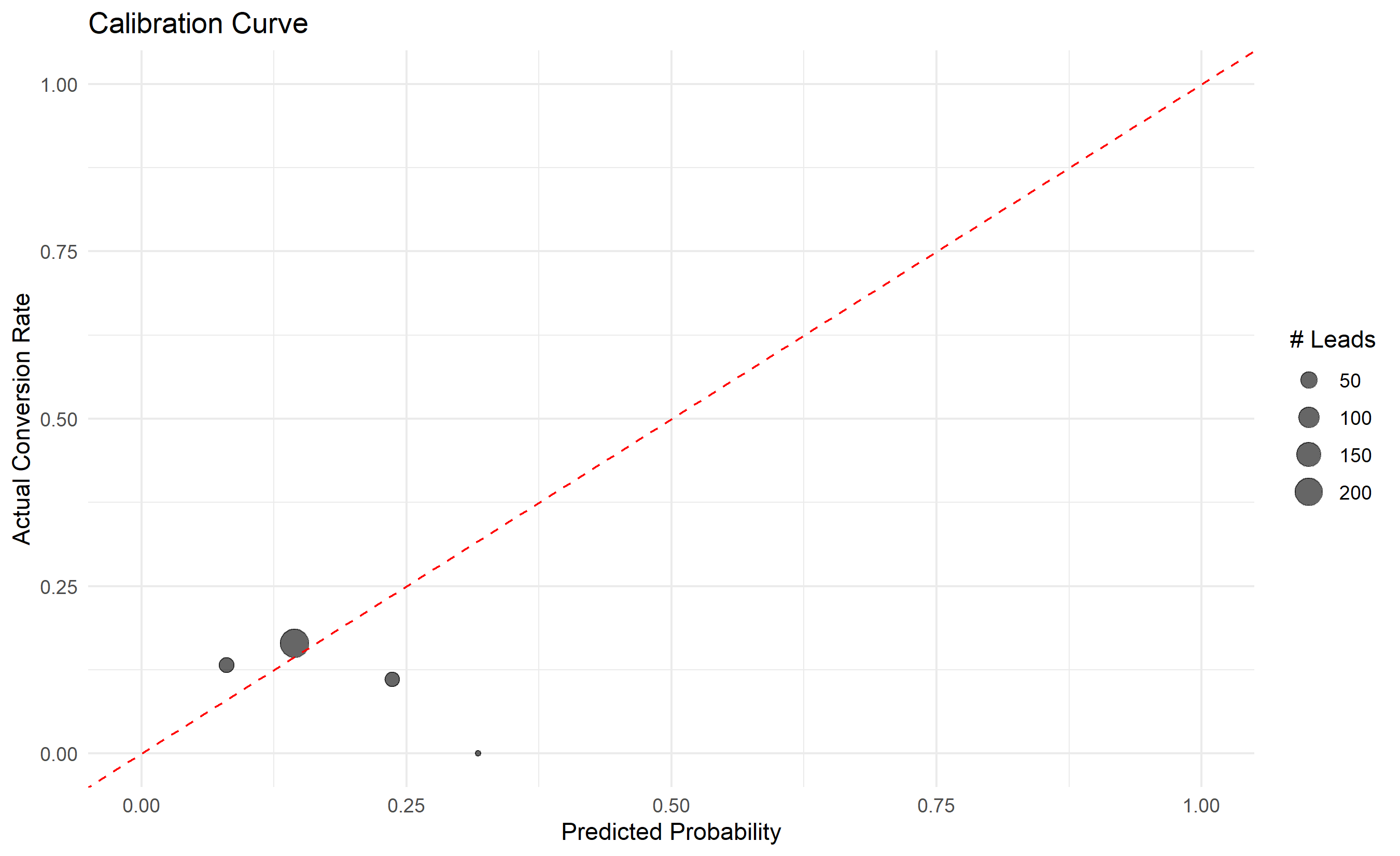
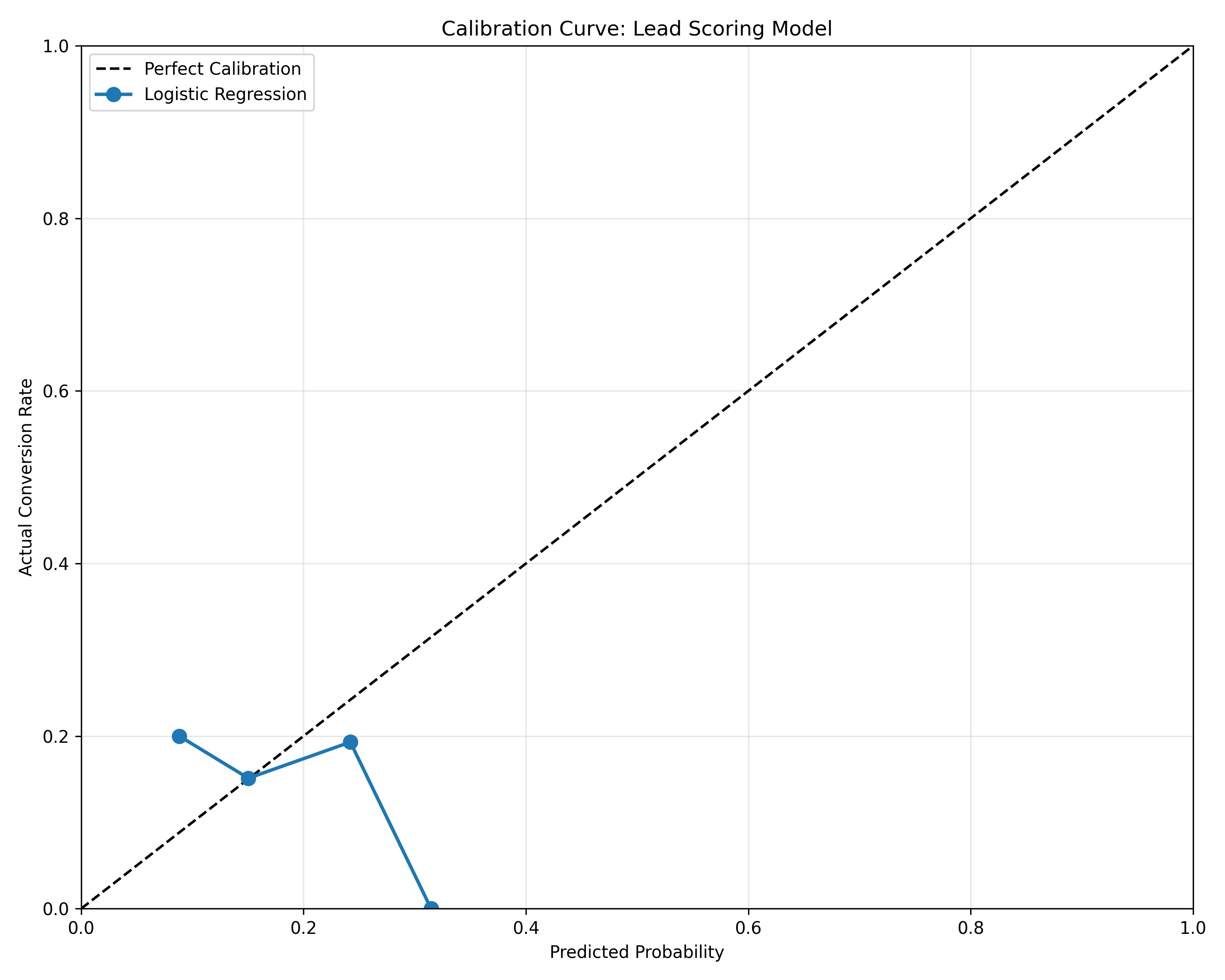
1. What does a calibration curve show? Why is it important?
2. If predicted probability is 0.4 but actual conversion rate is 0.6, what does this indicate?
3. How would you use feature coefficients to explain to a sales leader why a lead is prioritized?
4. Why is logistic regression preferred over XGBoost for lead scoring?
:::
## Threshold and Tier Selection: Converting Probability to Action
A predicted probability (0.3, 0.5, 0.7) is not directly actionable. We must convert it to a **tier** (Hot/Warm/Cold) with a corresponding **action** (sales call, nurture email, etc.).
::: {.callout-note icon="false"}
## 📘 Theory: Threshold Selection for Business Value
**Cost-benefit framework:**
- True Positive (Sales pursues, lead converts): +$X revenue.
- False Positive (Sales pursues, lead doesn't convert): -$Y cost (sales time).
- False Negative (Sales doesn't pursue, lead converts): -$Z opportunity cost.
- True Negative (Sales doesn't pursue, lead doesn't convert): $0 (no cost, no benefit).
**Expected value per prediction at threshold t:**
$$EV(t) = P(\text{TP}|t) \cdot X + P(\text{FP}|t) \cdot (-Y) + P(\text{FN}|t) \cdot (-Z)$$
Choose t to **maximize expected value**.
**In practice:**
1. **Estimate costs from business** (what's the cost of a sales call? typical deal value?).
2. **Compute expected value across thresholds** using confusion matrices.
3. **Select threshold** that maximizes EV.
4. **Define tiers** using evenly-spaced probabilities or cost-based thresholds.
**Precision-recall trade-off:**
- **High threshold:** Few leads flagged as Hot (high precision, low recall). Sales team doesn't get false alarms but misses opportunities.
- **Low threshold:** Many leads flagged as Hot (low precision, high recall). Sales pursues more but wastes time on unlikely converts.
:::
::: {.callout-tip icon="false"}
## 🔑 Key Formula: Expected Value Optimization
$$\text{Optimal Threshold} = \arg\max_t \left[ P(\text{TP}|t) \cdot Value - P(\text{FP}|t) \cdot Cost \right]$$
:::
### Threshold Selection and Tier Assignment
::: {.panel-tabset}
## R
```{r}
# Threshold selection based on ROI
# Assume costs/values
deal_value <- 100000 # ₦100,000 average deal
sales_cost_per_hour <- 500 # ₦500/hr
hours_per_lead <- 5 # 5 hours to qualify a lead
total_sales_cost <- sales_cost_per_hour * hours_per_lead # ₦2,500
# Compute expected value across thresholds
thresholds <- seq(0.1, 0.9, by = 0.05)
ev_results <- data.frame()
get_cm <- function(cm, row, col) {
if (row %in% rownames(cm) && col %in% colnames(cm)) cm[row, col] else 0L
}
for (t in thresholds) {
pred_class <- as.integer(pred_test >= t)
cm <- table(Actual = y_test, Predicted = pred_class)
tn <- get_cm(cm, "0", "0")
fp <- get_cm(cm, "0", "1")
fn <- get_cm(cm, "1", "0")
tp <- get_cm(cm, "1", "1")
# Expected value
ev <- (tp * deal_value) - (fp * total_sales_cost) - (fn * deal_value * 0.1) # 10% opportunity cost
ev_results <- rbind(ev_results, data.frame(
threshold = t,
tp = tp,
fp = fp,
fn = fn,
precision = tp / (tp + fp + 0.001),
recall = tp / (tp + fn + 0.001),
ev = ev
))
}
cat("Threshold Optimization Results:\n")
print(ev_results |> arrange(desc(ev)) |> head(5))
optimal_threshold <- ev_results$threshold[which.max(ev_results$ev)]
cat("\nOptimal threshold:", optimal_threshold, "\n")
# Define tiers based on threshold
leads_with_scores <- data.frame(
lead_id = leads_engineered$lead_id[-train_idx],
predicted_prob = pred_test,
actual = y_test
) |>
mutate(
tier = case_when(
predicted_prob >= optimal_threshold ~ "Hot",
predicted_prob >= optimal_threshold * 0.6 ~ "Warm",
TRUE ~ "Cold"
)
)
# Tier statistics
cat("\n## Lead Tier Distribution and Performance ##\n")
tier_stats <- leads_with_scores |>
group_by(tier) |>
summarise(
n_leads = n(),
pct_total = n() / nrow(leads_with_scores) * 100,
conversion_rate = mean(actual),
avg_score = mean(predicted_prob)
)
print(tier_stats)
# Expected revenue
cat("\n## Expected Revenue by Tier ##\n")
revenue_by_tier <- tier_stats |>
mutate(
expected_conversions = n_leads * conversion_rate,
expected_revenue = expected_conversions * deal_value,
investigation_cost = n_leads * total_sales_cost,
net_revenue = expected_revenue - investigation_cost
)
print(revenue_by_tier |> select(tier, expected_conversions, expected_revenue, investigation_cost, net_revenue))
```
## Python
```{python}
# Threshold selection based on cost-benefit
from sklearn.metrics import confusion_matrix
# Business parameters
deal_value = 100000 # ₦100,000
sales_cost_per_hour = 500
hours_per_lead = 5
total_sales_cost = sales_cost_per_hour * hours_per_lead # ₦2,500
# Compute EV across thresholds
thresholds = np.arange(0.1, 0.95, 0.05)
ev_results = []
for t in thresholds:
pred_class = (pred_test >= t).astype(int)
cm = confusion_matrix(y_test, pred_class, labels=[0, 1])
tn, fp, fn, tp = cm.ravel()
# Expected value
ev = (tp * deal_value) - (fp * total_sales_cost) - (fn * deal_value * 0.1)
precision = tp / (tp + fp + 0.001)
recall = tp / (tp + fn + 0.001)
ev_results.append({
'threshold': t,
'tp': tp,
'fp': fp,
'fn': fn,
'precision': precision,
'recall': recall,
'ev': ev
})
ev_df = pd.DataFrame(ev_results)
print("Threshold Optimization Results (Top 5):")
print(ev_df.nlargest(5, 'ev')[['threshold', 'tp', 'fp', 'ev']])
optimal_threshold = ev_df.loc[ev_df['ev'].idxmax(), 'threshold']
print(f"\nOptimal Threshold: {optimal_threshold:.2f}")
# Assign tiers
leads_with_scores = pd.DataFrame({
'lead_id': leads_engineered.iloc[-len(y_test):]['lead_id'].values,
'predicted_prob': pred_test,
'actual': y_test.values
})
leads_with_scores['tier'] = pd.cut(
leads_with_scores['predicted_prob'],
bins=[0, optimal_threshold * 0.6, optimal_threshold, 1.0],
labels=['Cold', 'Warm', 'Hot'],
include_lowest=True
)
print("\n## Lead Tier Distribution and Performance ##")
tier_stats = leads_with_scores.groupby('tier').agg({
'predicted_prob': 'count',
'actual': 'mean'
}).rename(columns={'predicted_prob': 'n_leads', 'actual': 'conversion_rate'})
tier_stats['pct_total'] = tier_stats['n_leads'] / len(leads_with_scores) * 100
tier_stats = tier_stats.reset_index()
print(tier_stats)
# Revenue impact
print("\n## Expected Revenue by Tier ##")
revenue_df = tier_stats.copy()
revenue_df['expected_conversions'] = revenue_df['n_leads'] * revenue_df['conversion_rate']
revenue_df['expected_revenue'] = revenue_df['expected_conversions'] * deal_value
revenue_df['investigation_cost'] = revenue_df['n_leads'] * total_sales_cost
revenue_df['net_revenue'] = revenue_df['expected_revenue'] - revenue_df['investigation_cost']
print(revenue_df[['tier', 'expected_conversions', 'expected_revenue', 'investigation_cost', 'net_revenue']])
```
:::
::: {.callout-caution icon="false"}
## 📝 Section 17.5 Review Questions
1. In the cost-benefit framework, what is "opportunity cost"? How would you estimate it?
2. If sales cost per lead is ₦2,500 but deal value is ₦100,000, why pursue any low-probability leads?
3. How would you adjust tier thresholds if the sales team's capacity doubles?
4. What is the "precision-recall trade-off" in lead scoring?
:::
## Deploying and Monitoring Lead Scores
Once in production, scores drift as market conditions change. **Population Stability Index (PSI)** detects drift.
::: {.callout-note icon="false"}
## 📘 Theory: Population Stability Index (PSI)
**Motivation:**
A model trained on 2026 leads may not predict 2027 leads if buyer behavior shifts. We monitor this with PSI.
**Definition:**
$$PSI = \sum_{i=1}^{n} (P_i^{actual} - P_i^{expected}) \log\left(\frac{P_i^{actual}}{P_i^{expected}}\right)$$
where:
- Divide predictions into n bins (e.g., deciles).
- $P_i^{expected}$ is the frequency of bin i in training data.
- $P_i^{actual}$ is the frequency of bin i in recent data (e.g., last month).
**Interpretation:**
- PSI < 0.1: No significant shift (all is well).
- PSI 0.1–0.25: Small shift (monitor).
- PSI > 0.25: Large shift (retrain model).
**Deployment workflow:**
1. Train model on historical data.
2. Score all new leads daily/weekly.
3. Compute PSI monthly.
4. If PSI > 0.25, flag for retraining.
5. Retrain on latest data (last 6–12 months).
:::
### Monitoring Script
::: {.panel-tabset}
## R
```{r}
# Population Stability Index
compute_psi <- function(expected, actual, bins = 10) {
# Binning
breaks <- quantile(expected, probs = seq(0, 1, 1/bins))
breaks[1] <- -Inf
breaks[length(breaks)] <- Inf
expected_bin <- cut(expected, breaks = breaks)
actual_bin <- cut(actual, breaks = breaks)
# Frequencies
expected_freq <- table(expected_bin) / length(expected)
actual_freq <- table(actual_bin) / length(actual)
# Ensure same bins
all_bins <- union(names(expected_freq), names(actual_freq))
expected_freq <- expected_freq[all_bins]
actual_freq <- actual_freq[all_bins]
expected_freq[is.na(expected_freq) | expected_freq == 0] <- 0.0001
actual_freq[is.na(actual_freq) | actual_freq == 0] <- 0.0001
# PSI
psi <- sum((actual_freq - expected_freq) * log(actual_freq / expected_freq))
return(psi)
}
# Simulate model drift: 2026 baseline vs. 2027 data
set.seed(2026)
baseline_scores <- pred_test # 2026 data
# Simulate 2027 data with drift (leads are easier/harder to convert)
drift_scores <- baseline_scores + rnorm(length(baseline_scores), mean = 0.1, sd = 0.05)
drift_scores <- pmax(0, pmin(1, drift_scores)) # Bound to [0, 1]
# Compute PSI
psi_value <- compute_psi(baseline_scores, drift_scores)
cat("=== MONITORING: POPULATION STABILITY INDEX ===\n\n")
cat("Baseline (2026) mean score:", round(mean(baseline_scores), 4), "\n")
cat("Recent (2027) mean score:", round(mean(drift_scores), 4), "\n")
cat("PSI:", round(psi_value, 4), "\n\n")
if (psi_value < 0.1) {
status <- "✓ No drift (PSI < 0.1)"
} else if (psi_value < 0.25) {
status <- "⚠ Minor drift (0.1 ≤ PSI < 0.25): Monitor"
} else {
status <- "✗ Major drift (PSI ≥ 0.25): Retrain recommended"
}
cat("Status:", status, "\n")
```
## Python
```{python}
def compute_psi(expected, actual, bins=10):
"""Compute Population Stability Index."""
# Binning
breaks = np.percentile(expected, np.linspace(0, 100, bins + 1))
breaks[0] = -np.inf
breaks[-1] = np.inf
expected_bin = np.digitize(expected, breaks)
actual_bin = np.digitize(actual, breaks)
# Frequencies
expected_freq = np.bincount(expected_bin) / len(expected)
actual_freq = np.bincount(actual_bin) / len(actual)
# Ensure same length
max_len = max(len(expected_freq), len(actual_freq))
expected_freq = np.pad(expected_freq, (0, max_len - len(expected_freq)), constant_values=0.0001)
actual_freq = np.pad(actual_freq, (0, max_len - len(actual_freq)), constant_values=0.0001)
# Replace zeros with small epsilon to avoid log(0)
expected_freq = np.where(expected_freq == 0, 0.0001, expected_freq)
actual_freq = np.where(actual_freq == 0, 0.0001, actual_freq)
# PSI
psi = np.sum((actual_freq - expected_freq) * np.log(actual_freq / expected_freq))
return psi
# Simulate drift
np.random.seed(2026)
baseline_scores = pred_test # 2026 baseline
# 2027 data with drift
drift_scores = baseline_scores + np.random.normal(0.1, 0.05, len(baseline_scores))
drift_scores = np.clip(drift_scores, 0, 1)
# Compute PSI
psi_value = compute_psi(baseline_scores, drift_scores)
print("=== MONITORING: POPULATION STABILITY INDEX ===\n")
print(f"Baseline (2026) mean score: {baseline_scores.mean():.4f}")
print(f"Recent (2027) mean score: {drift_scores.mean():.4f}")
print(f"PSI: {psi_value:.4f}\n")
if psi_value < 0.1:
status = "✓ No drift (PSI < 0.1)"
elif psi_value < 0.25:
status = "⚠ Minor drift (0.1 ≤ PSI < 0.25): Monitor"
else:
status = "✗ Major drift (PSI ≥ 0.25): Retrain recommended"
print(f"Status: {status}")
```
:::
::: {.callout-caution icon="false"}
## 📝 Section 17.6 Review Questions
1. What are typical causes of score drift in lead scoring?
2. If PSI = 0.15, what action would you take?
3. How frequently should you monitor PSI in production?
4. What data should you use to retrain after drift detection?
:::
## Case Study: B2B Lead Scoring for a Pan-African Fintech
Complete pipeline: data preprocessing → feature engineering → model training → threshold tuning → business recommendations.
::: {.panel-tabset}
## R
```{r}
cat("=== CASE STUDY: B2B LEAD SCORING FOR PAN-AFRICAN FINTECH ===\n\n")
cat("## Step 1: Data Summary ##\n")
cat("Total leads:", nrow(leads_engineered), "\n")
cat("Conversions:", sum(leads_engineered$converted), "\n")
cat("Base conversion rate:", round(mean(leads_engineered$converted), 4), "\n\n")
cat("## Step 2: Model Performance ##\n")
cat("Test AUC:", round(as.numeric(auc_test), 4), "\n")
cat("Brier Score:", round(mean((pred_test - y_test)^2), 4), "\n\n")
# Top features
lr_coefs <- coef(lr_model)[-1] # Exclude intercept
top_features <- names(sort(abs(lr_coefs), decreasing = TRUE)[1:5])
cat("## Step 3: Top 5 Most Predictive Features ##\n")
for (feat in top_features) {
cat(sprintf("%s: %+.4f (Odds Ratio: %.2f)\n",
feat,
lr_coefs[feat],
exp(lr_coefs[feat])))
}
cat("\n## Step 4: Lead Tier Analysis ##\n")
print(tier_stats)
cat("\n## Step 5: Business Recommendations ##\n")
# Top Hot leads for immediate pursuit
top_hot_leads <- leads_with_scores |>
filter(tier == "Hot") |>
arrange(desc(predicted_prob)) |>
head(10)
cat("\nTop 10 Hot leads (ready for sales outreach):\n")
print(top_hot_leads |> select(lead_id, predicted_prob, tier))
# Revenue opportunity
total_hot_revenue <- revenue_by_tier |>
filter(tier == "Hot") |>
pull(expected_revenue)
total_warm_revenue <- revenue_by_tier |>
filter(tier == "Warm") |>
pull(expected_revenue)
cat(sprintf("\nRevenue Opportunity:\n"))
cat(sprintf(" Hot tier (immediate pursuit): ₦%.0f\n", total_hot_revenue))
cat(sprintf(" Warm tier (nurture track): ₦%.0f\n", total_warm_revenue))
cat(sprintf(" Total potential: ₦%.0f\n\n", total_hot_revenue + total_warm_revenue))
# Sales allocation
hot_leads_count <- tier_stats |> filter(tier == "Hot") |> pull(n_leads)
cat(sprintf("Recommended Sales Allocation:\n"))
cat(sprintf(" Assign %d sales reps to %d Hot leads (%.1f leads/rep)\n",
ceiling(hot_leads_count / 20), hot_leads_count, hot_leads_count / ceiling(hot_leads_count / 20)))
cat("\n## Step 6: Deployment Checklist ##\n")
cat("[ ] Model integrated into CRM\n")
cat("[ ] Scores refresh daily\n")
cat("[ ] PSI monitoring active (threshold: 0.25)\n")
cat("[ ] Sales team trained on tier definitions\n")
cat("[ ] Feedback loop: track conversion vs. prediction\n")
cat("[ ] Retrain schedule: quarterly (or when PSI > 0.25)\n")
```
## Python
```{python}
print("=" * 70)
print("CASE STUDY: B2B LEAD SCORING FOR PAN-AFRICAN FINTECH")
print("=" * 70)
print()
print("## Step 1: Data Summary ##")
print(f"Total leads: {len(leads_engineered)}")
print(f"Conversions: {leads_engineered['converted'].sum()}")
print(f"Base conversion rate: {leads_engineered['converted'].mean():.4f}\n")
print("## Step 2: Model Performance ##")
print(f"Test AUC: {auc_test:.4f}")
print(f"Brier Score: {brier_test:.4f}\n")
print("## Step 3: Top 5 Most Predictive Features ##")
top_coef = coef_df.head(5)
for _, row in top_coef.iterrows():
print(f"{row['Feature']}: {row['Coefficient']:+.4f} (Odds Ratio: {row['Odds Ratio']:.2f})")
print("\n## Step 4: Lead Tier Analysis ##")
print(tier_stats.to_string(index=False))
print("\n## Step 5: Business Recommendations ##")
top_hot = leads_with_scores[leads_with_scores['tier'] == 'Hot'].nlargest(10, 'predicted_prob')
print("\nTop 10 Hot leads (ready for sales outreach):")
print(top_hot[['lead_id', 'predicted_prob', 'tier']].to_string(index=False))
hot_revenue = revenue_df[revenue_df['tier'] == 'Hot']['expected_revenue'].sum()
warm_revenue = revenue_df[revenue_df['tier'] == 'Warm']['expected_revenue'].sum()
print(f"\nRevenue Opportunity:")
print(f" Hot tier (immediate pursuit): ₦{hot_revenue:,.0f}")
print(f" Warm tier (nurture track): ₦{warm_revenue:,.0f}")
print(f" Total potential: ₦{hot_revenue + warm_revenue:,.0f}\n")
hot_count = (leads_with_scores['tier'] == 'Hot').sum()
reps_needed = max(1, hot_count // 20)
print(f"Recommended Sales Allocation:")
print(f" Assign {reps_needed} sales reps to {hot_count} Hot leads ({hot_count / reps_needed:.1f} leads/rep)")
print("\n## Step 6: Deployment Checklist ##")
print("[ ] Model integrated into CRM")
print("[ ] Scores refresh daily")
print("[ ] PSI monitoring active (threshold: 0.25)")
print("[ ] Sales team trained on tier definitions")
print("[ ] Feedback loop: track conversion vs. prediction")
print("[ ] Retrain schedule: quarterly (or when PSI > 0.25)")
```
:::
::: {.callout-caution icon="false"}
## 📝 Section 17.7 Review Questions
1. In the case study, what is the expected revenue impact of the lead scoring system?
2. How would you adjust tier thresholds if sales team feedback suggests too many false positives?
3. What would you do if 6 months later, PSI = 0.28?
:::
## Chapter 17 Exercises
::: {.exercises}
1. **Feature engineering:** Create 10 new features for lead scoring from raw CRM data.
2. **Threshold optimization:** Calculate optimal threshold using precision-recall trade-off (F1 score).
3. **Tiering strategy:** Define 4 tiers (Platinum, Gold, Silver, Bronze) with different nurture actions.
4. **ROI calculation:** Estimate the revenue lift from lead scoring (conversion rate improvement × deal volume).
5. **Calibration analysis:** Plot calibration curves for different feature sets; which is best calibrated?
6. **Segment analysis:** Build separate models for different sectors (fintech vs. e-commerce). Do they differ?
7. **Champion-challenger test:** A/B test the new lead scoring model against the old approach for 1 month.
8. **CRM integration:** Design an API contract for scoring leads in real-time.
9. **Fairness audit:** Check if score distributions are similar across geographies (bias check).
10. **Long-term tracking:** Score leads now, follow up in 6 months to measure conversion rate vs. prediction.
:::
## Further Reading
1. **Blattberg, R. C., Kim, B. D., & Neslin, S. A.** (2008). *Database Marketing: Analyzing and Managing Customers*. Springer. — Classic reference on customer lifetime value and scoring.
2. **James, G., Witten, D., Hastie, T., & Tibshirani, R.** (2013). *An Introduction to Statistical Learning*. Springer. — Chapter on logistic regression and classification.
3. **Naeem Siddiqi.** (2006). *Credit Risk Scorecards: Developing and Implementing Intelligent Credit Scoring*. John Wiley & Sons. — Detailed guide to scorecard building.
4. **Verbeke, W., Martens, D., & Baesens, B.** (2011). "Social network analysis for customer churn prediction." *Journal of the Operational Research Society*, 62(1), 28–46. — Network effects in churn prediction.
5. **Kaggle Lead Scoring Competitions.** [https://www.kaggle.com] — Real-world lead scoring datasets and solutions.
## Chapter 17 Appendix
### A. Platt Scaling for Probability Calibration
If a model's predicted probabilities are poorly calibrated (e.g., always too high), we can apply **Platt scaling**: fit a logistic regression on the model's outputs.
**Before calibration:**
$$\hat{p} = f_{model}(x)$$
**Platt scaling:**
$$\hat{p}_{calibrated} = \frac{1}{1 + e^{-(a \cdot \hat{p} + b)}}$$
Estimate a, b on a hold-out validation set by fitting logistic regression with $\hat{p}$ as input and true y as output.
**Advantages:**
- Simple, interpretable.
- Preserves AUC (only shifts probabilities).
**Disadvantage:**
- Requires additional hold-out data.
### B. Isotonic Regression for Calibration
For non-monotonic miscalibration, **isotonic regression** is more flexible:
$$y_{cal} = f_{iso}(\hat{p})$$
where $f_{iso}$ is a monotonically increasing function fit to minimize residuals. This requires more data but is less restrictive than Platt scaling.
### C. Population Stability Index: Alternative Interpretation
PSI can be decomposed into two components:
$$PSI = \underbrace{\sum (P_i^{actual} - P_i^{expected}) \log(P_i^{actual})}_{\text{Distribution shift}} + \underbrace{\sum (P_i^{expected} - P_i^{actual}) \log(P_i^{expected})}_{\text{Reference shift}}$$
This separates changes in the distribution from changes in the reference baseline, helping diagnose whether drift is due to new lead characteristics or model miscalibration.
---
*End of Chapter 17*