19 Decision Trees – AI-Powered Business Analytics

19.1 The Decision Tree Metaphor

A decision tree is a flowchart that asks a series of yes/no questions to reach a final decision. Imagine a bank manager deciding whether to approve a loan:

“Is the applicant’s annual income above ₦5 million?” → Yes → Next question “Is their debt-to-income ratio below 0.4?” → Yes → Approve “Has the applicant been employed for at least 2 years?” → Yes → Approve “No?” → Reject

This intuitive process of asking sequential binary questions is exactly what a decision tree does. Each question partitions the data into smaller subsets, and we repeat until we reach a pure subset (all yes, all no) or stop by rule.

📘 Theory: Anatomy of a Decision Tree

Nodes: - Root node: The top node where all data starts. It asks the first question.

Internal nodes: Intermediate nodes that ask splitting questions. Each has one parent and two children.
Leaf nodes: Terminal nodes with no children. They assign a final class or prediction (e.g., “Approve”, “Reject”, “Fraud”).

Edges (Branches): - Each branch represents the outcome of a yes/no question (left for “no,” right for “yes”).

Every path from root to leaf defines a decision rule that can be explained to a non-technical person.

Why trees are interpretable: A single prediction path reads like: “Customer has income > ₦10M AND has existing account AND has zero defaults → Approved.”

This is far more transparent than a neural network’s 50 hidden layers. Decision trees satisfy regulatory demands (especially in financial services) to explain decisions to customers.

19.1.1 Reading a Decision Tree

📝 Section 14.1 Review Questions

What is the relationship between a decision tree flowchart and a bank manager’s loan approval process?
Define root node, internal node, and leaf node. What does each do?
How does a decision rule in a tree translate into a customer-facing explanation?
Why do regulators prefer decision trees over black-box models like neural networks?

19.2 Splitting Criteria: Information Gain and Gini Impurity

The core question is: Which feature and threshold should we use to split at each node? We need a criterion that measures how much purer the resulting child nodes are compared to the parent.

📘 Theory: Impurity Measures

Entropy (Information Gain): Entropy measures the disorder in a node. A node is pure if all samples belong to one class; impure if samples are mixed.

\[H(S) = -\sum_{i=1}^{C} p_i \log_2(p_i)\]

where \(p_i\) is the fraction of samples of class \(i\) in set \(S\), and \(C\) is the number of classes.

Properties:

H(S) = 0 if all samples are one class (pure).
H(S) is maximum when all classes are equally represented (maximum uncertainty).
For binary classification: \(H = -p \log_2(p) - (1-p) \log_2(1-p)\), maximized at p = 0.5.

Information Gain (IG): IG measures the reduction in entropy after a split. A split on feature \(X_j\) at threshold \(t\) divides set \(S\) into \(S_L\) (left, X_j ≤ t) and \(S_R\) (right, X_j > t).

\[IG(S, X_j, t) = H(S) - \frac{|S_L|}{|S|} H(S_L) - \frac{|S_R|}{|S|} H(S_R)\]

We choose the split that maximizes IG.

Gini Impurity: An alternative impurity measure, particularly popular in CART (Classification And Regression Trees):

\[Gini(S) = 1 - \sum_{i=1}^{C} p_i^2\]

Gini ranges from 0 (pure) to 1 − 1/C (maximum impurity). For binary: \(Gini = 2p(1-p)\).

IG vs. Gini: - Both lead to similar trees in practice. - Gini is faster to compute (no logarithms). - IG is more interpretable (measured in bits). - Gini is used by scikit-learn’s DecisionTreeClassifier by default.

For regression trees: Instead of entropy, we use variance reduction. At each node, compute the within-group variance of y values. A split is good if it reduces the weighted variance in the children.

\[\text{Var}_{reduction} = Var(S) - \frac{|S_L|}{|S|} Var(S_L) - \frac{|S_R|}{|S|} Var(S_R)\]

🔑 Key Formula: Information Gain and Gini

Entropy: \[H(S) = -\sum_{i=1}^{C} p_i \log_2(p_i)\]

Gini Impurity: \[Gini(S) = 1 - \sum_{i=1}^{C} p_i^2\]

Information Gain (entropy-based): \[IG(S, X_j, t) = H(S) - \frac{|S_L|}{|S|} H(S_L) - \frac{|S_R|}{|S|} H(S_R)\]

Variance Reduction (regression): \[VarRed(S, X_j, t) = Var(S) - \frac{|S_L|}{|S|} Var(S_L) - \frac{|S_R|}{|S|} Var(S_R)\]

19.2.1 Computing Gini and Entropy by Hand

Let’s work through a simple example. Suppose we have 10 insurance claims: - 7 are legitimate (class 0) - 3 are fraudulent (class 1)

Parent node entropy: \[H = -0.7 \log_2(0.7) - 0.3 \log_2(0.3) = -0.7(−0.515) - 0.3(−1.737) = 0.361 + 0.521 = 0.882\]

Parent node Gini: \[Gini = 1 - (0.7)^2 - (0.3)^2 = 1 - 0.49 - 0.09 = 0.42\]

Now suppose we split on claim_amount ≤ ₦500,000: - Left (≤ ₦500k): 6 samples: 5 legitimate, 1 fraudulent - Right (> ₦500k): 4 samples: 2 legitimate, 2 fraudulent

Left entropy: \(H_L = -\frac{5}{6}\log_2(\frac{5}{6}) - \frac{1}{6}\log_2(\frac{1}{6}) = 0.277 + 0.389 = 0.666\)

Right entropy: \(H_R = -0.5 \log_2(0.5) - 0.5 \log_2(0.5) = 1.0\)

Information gain: \[IG = 0.882 - \frac{6}{10}(0.666) - \frac{4}{10}(1.0) = 0.882 - 0.400 - 0.400 = 0.082\]

This split reduces impurity by 0.082 bits.

Show code

library(tidyverse)

# Function to compute entropy
entropy <- function(p) {
  p <- p[p > 0 & p < 1]  # Remove 0s and 1s to avoid log(0)
  -sum(p * log2(p))
}

# Function to compute Gini
gini <- function(p) {
  1 - sum(p^2)
}

# Example: 10 claims, 7 legitimate, 3 fraudulent
class_counts <- c(7, 3)
total <- sum(class_counts)
p <- class_counts / total

cat("Parent node:\n")
#> Parent node:
cat("Entropy:", entropy(p), "\n")
#> Entropy: 0.8812909
cat("Gini:", gini(p), "\n\n")
#> Gini: 0.42

# After split on claim_amount <= 500,000
left_counts <- c(5, 1)   # 5 legitimate, 1 fraudulent
right_counts <- c(2, 2)  # 2 legitimate, 2 fraudulent

left_p <- left_counts / sum(left_counts)
right_p <- right_counts / sum(right_counts)

left_ent <- entropy(left_p)
right_ent <- entropy(right_p)
left_gini <- gini(left_p)
right_gini <- gini(right_p)

parent_ent <- entropy(p)
parent_gini <- gini(p)

# Weighted entropy and Gini after split
weighted_ent <- (6/10) * left_ent + (4/10) * right_ent
weighted_gini <- (6/10) * left_gini + (4/10) * right_gini

cat("After split on claim_amount <= 500,000:\n")
#> After split on claim_amount <= 500,000:
cat("Left child (n=6): Entropy =", round(left_ent, 3), ", Gini =", round(left_gini, 3), "\n")
#> Left child (n=6): Entropy = 0.65 , Gini = 0.278
cat("Right child (n=4): Entropy =", round(right_ent, 3), ", Gini =", round(right_gini, 3), "\n\n")
#> Right child (n=4): Entropy = 1 , Gini = 0.5

cat("Information Gain (Entropy):", round(parent_ent - weighted_ent, 3), "\n")
#> Information Gain (Entropy): 0.091
cat("Gini Gain:", round(parent_gini - weighted_gini, 3), "\n")
#> Gini Gain: 0.053

Show code

import numpy as np
from scipy.stats import entropy as scipy_entropy

def compute_entropy(class_counts):
    """Compute entropy given class counts."""
    total = np.sum(class_counts)
    p = class_counts / total
    # Entropy in bits (log2)
    ent = -np.sum(p[p > 0] * np.log2(p[p > 0]))
    return ent

def compute_gini(class_counts):
    """Compute Gini impurity given class counts."""
    total = np.sum(class_counts)
    p = class_counts / total
    gini = 1 - np.sum(p**2)
    return gini

# Parent node: 7 legitimate, 3 fraudulent
parent_counts = np.array([7, 3])
parent_ent = compute_entropy(parent_counts)
parent_gini = compute_gini(parent_counts)

print("Parent node:")
#> Parent node:
print(f"  Entropy: {parent_ent:.4f}")
#>   Entropy: 0.8813
print(f"  Gini: {parent_gini:.4f}\n")
#>   Gini: 0.4200

# Split: claim_amount <= 500,000
left_counts = np.array([5, 1])   # 5 legitimate, 1 fraudulent
right_counts = np.array([2, 2])  # 2 legitimate, 2 fraudulent

left_ent = compute_entropy(left_counts)
right_ent = compute_entropy(right_counts)
left_gini = compute_gini(left_counts)
right_gini = compute_gini(right_counts)

n_left = np.sum(left_counts)
n_right = np.sum(right_counts)
n_total = n_left + n_right

weighted_ent = (n_left / n_total) * left_ent + (n_right / n_total) * right_ent
weighted_gini = (n_left / n_total) * left_gini + (n_right / n_total) * right_gini

ig = parent_ent - weighted_ent
gini_gain = parent_gini - weighted_gini

print("After split on claim_amount <= 500,000:")
#> After split on claim_amount <= 500,000:
print(f"  Left (n={n_left}): Entropy={left_ent:.4f}, Gini={left_gini:.4f}")
#>   Left (n=6): Entropy=0.6500, Gini=0.2778
print(f"  Right (n={n_right}): Entropy={right_ent:.4f}, Gini={right_gini:.4f}\n")
#>   Right (n=4): Entropy=1.0000, Gini=0.5000
print(f"Information Gain (Entropy-based): {ig:.4f}")
#> Information Gain (Entropy-based): 0.0913
print(f"Gini Gain: {gini_gain:.4f}")
#> Gini Gain: 0.0533

📝 Section 14.2 Review Questions

Why is entropy 0 at a leaf node with all samples of one class?
Compute entropy and Gini for a node with 100 samples: 50 class A, 50 class B.
If a split results in IG = 0.05 bits, is this a good or bad split? How do you decide?
For regression trees, what impurity measure replaces entropy?
Given a fraudulent claim is much rarer than legitimate claims, does information gain favour splits that isolate fraud?

19.3 Growing a Full Tree: The CART Algorithm

The CART (Classification and Regression Trees) algorithm grows a tree greedily:

Start with all data at the root node.
For each node, evaluate all possible binary splits on all features.
Choose the split that maximizes information gain (or Gini gain for CART).
Recursively apply steps 2–3 to the resulting child nodes.
Stop when a stopping criterion is met (e.g., min samples per leaf, max depth, no improvement).

📘 Theory: The CART Algorithm

Algorithm:

function GROW_TREE(S, depth):
    if stopping_criterion(S, depth) or is_pure(S):
        return LEAF_NODE(majority_class(S))

    best_gain = -∞
    best_split = None

    for each feature j and threshold t:
        S_L = {(x, y) ∈ S : x_j ≤ t}
        S_R = {(x, y) ∈ S : x_j > t}

        gain = INFORMATION_GAIN(S, S_L, S_R)
        if gain > best_gain:
            best_gain = gain
            best_split = (j, t)

    S_L, S_R = apply_split(S, best_split)

    left_child = GROW_TREE(S_L, depth + 1)
    right_child = GROW_TREE(S_R, depth + 1)

    return INTERNAL_NODE(best_split, left_child, right_child)

Stopping criteria: - Minimum samples per leaf: Do not split if either child would have < min_samples_leaf observations. - Maximum depth: Do not split if depth >= max_depth. - Minimum impurity decrease: Do not split if the impurity decrease is < min_impurity_decrease (prevents trivial splits). - All samples same class: Node is pure; cannot improve.

Choosing thresholds: For continuous features, we evaluate all unique values in the data. For categorical features, we can: - One-vs-rest encoding: each category is one side of the split. - Ordinal encoding: if categories are ordered.

Why greedy? CART is a greedy algorithm: it makes locally optimal choices at each step. It does not backtrack. This means the final tree may not be globally optimal, but the algorithm is fast and works well in practice.

19.3.1 Case Study: Nigerian Insurance Fraud Detection

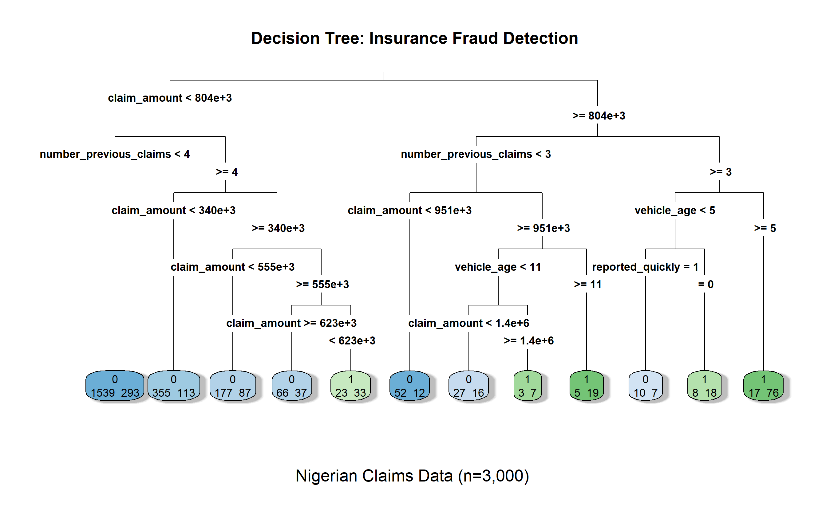
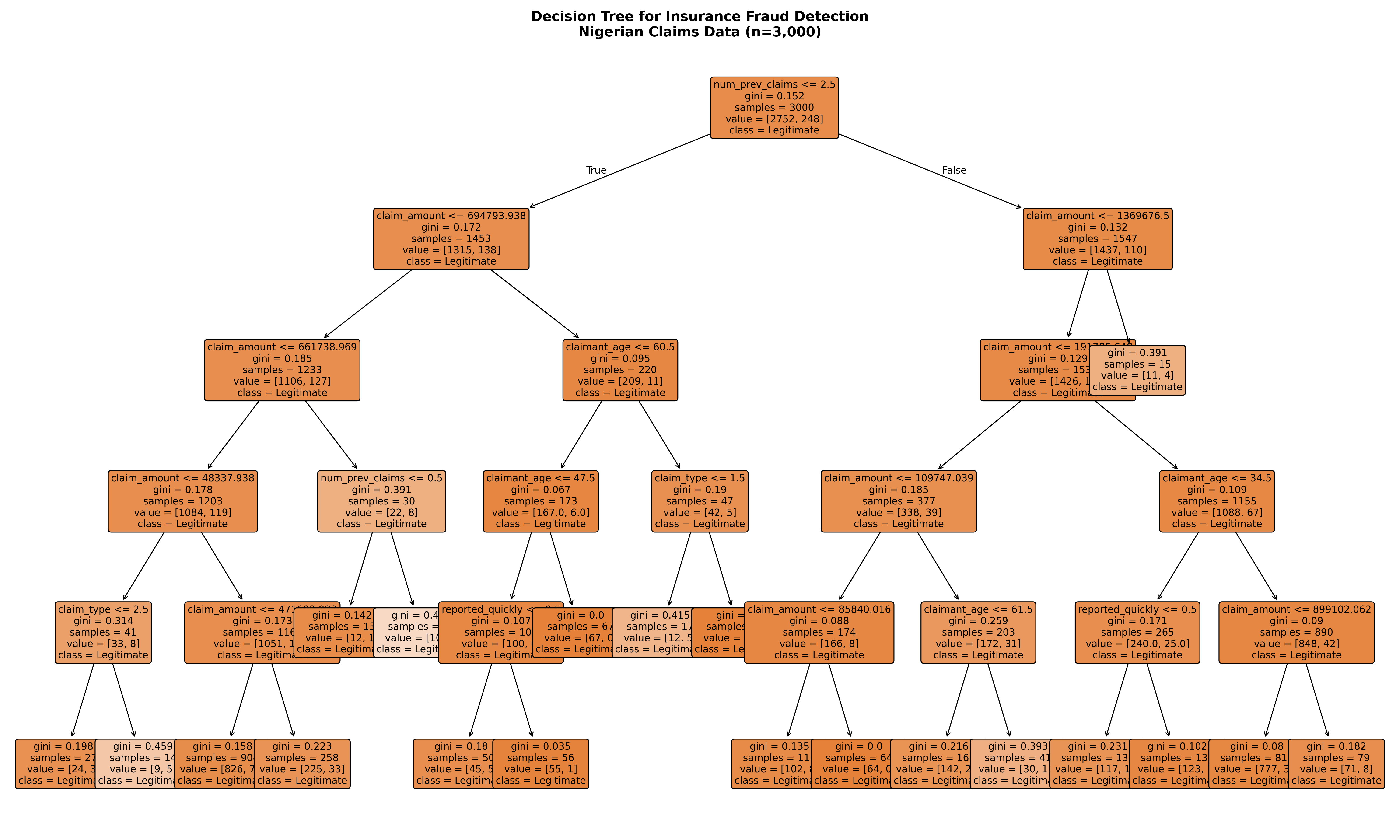
We’ll build a decision tree on a synthetic dataset of 3,000 insurance claims from Nigeria.

R

Show code

library(tidyverse)
library(rpart)
library(rpart.plot)

# Synthetic dataset: Nigerian insurance claims
set.seed(2026)
n_claims <- 3000

# Generate features first, then derive fraud probability from them
fraud_data <- tibble(
  claim_id               = 1:n_claims,
  claim_amount           = pmax(rgamma(n_claims, shape = 2, scale = 200000), 10000),
  claim_type             = sample(c("Vehicle", "Property", "Medical", "Liability"),
                                  n_claims, replace = TRUE,
                                  prob = c(0.5, 0.2, 0.15, 0.15)),
  claimant_age           = sample(25:70,  n_claims, replace = TRUE),
  vehicle_age            = sample(0:15,   n_claims, replace = TRUE),
  number_previous_claims = sample(0:5,    n_claims, replace = TRUE),
  reported_quickly       = sample(0:1,    n_claims, replace = TRUE)  # 1 = within 24 hours
) |>
  mutate(
    # Fraud probability driven by features so the tree can find real splits
    fraud_prob = plogis(-3 + 2e-6 * claim_amount +
                             0.3 * number_previous_claims -
                             0.6 * reported_quickly +
                             0.05 * vehicle_age),
    fraud = as.factor(rbinom(n_claims, 1, fraud_prob))
  ) |>
  select(-fraud_prob)

cat("Dataset shape:", nrow(fraud_data), "rows,", ncol(fraud_data), "columns\n")
#> Dataset shape: 3000 rows, 8 columns
cat("Fraud class distribution:\n")
#> Fraud class distribution:
print(table(fraud_data$fraud))
#> 
#>    0    1 
#> 2282  718

# Fit decision tree
dt_model <- rpart(
  fraud ~ claim_amount + claim_type + claimant_age + vehicle_age +
           number_previous_claims + reported_quickly,
  data    = fraud_data,
  method  = "class",
  control = rpart.control(minsplit = 20, minbucket = 10, cp = 0.001, maxdepth = 5)
)

cat("\nTree summary:\n")
#> 
#> Tree summary:
print(dt_model)
#> n= 3000 
#> 
#> node), split, n, loss, yval, (yprob)
#>       * denotes terminal node
#> 
#>  1) root 3000 718 0 (0.7606667 0.2393333)  
#>    2) claim_amount< 804132.1 2723 563 0 (0.7932427 0.2067573)  
#>      4) number_previous_claims< 3.5 1832 293 0 (0.8400655 0.1599345) *
#>      5) number_previous_claims>=3.5 891 270 0 (0.6969697 0.3030303)  
#>       10) claim_amount< 339502.9 468 113 0 (0.7585470 0.2414530) *
#>       11) claim_amount>=339502.9 423 157 0 (0.6288416 0.3711584)  
#>         22) claim_amount< 554614.3 264  87 0 (0.6704545 0.3295455) *
#>         23) claim_amount>=554614.3 159  70 0 (0.5597484 0.4402516)  
#>           46) claim_amount>=623141.9 103  37 0 (0.6407767 0.3592233) *
#>           47) claim_amount< 623141.9 56  23 1 (0.4107143 0.5892857) *
#>    3) claim_amount>=804132.1 277 122 1 (0.4404332 0.5595668)  
#>      6) number_previous_claims< 2.5 141  54 0 (0.6170213 0.3829787)  
#>       12) claim_amount< 951306.5 64  12 0 (0.8125000 0.1875000) *
#>       13) claim_amount>=951306.5 77  35 1 (0.4545455 0.5454545)  
#>         26) vehicle_age< 10.5 53  23 0 (0.5660377 0.4339623)  
#>           52) claim_amount< 1388589 43  16 0 (0.6279070 0.3720930) *
#>           53) claim_amount>=1388589 10   3 1 (0.3000000 0.7000000) *
#>         27) vehicle_age>=10.5 24   5 1 (0.2083333 0.7916667) *
#>      7) number_previous_claims>=2.5 136  35 1 (0.2573529 0.7426471)  
#>       14) vehicle_age< 4.5 43  18 1 (0.4186047 0.5813953)  
#>         28) reported_quickly>=0.5 17   7 0 (0.5882353 0.4117647) *
#>         29) reported_quickly< 0.5 26   8 1 (0.3076923 0.6923077) *
#>       15) vehicle_age>=4.5 93  17 1 (0.1827957 0.8172043) *

rpart.plot(dt_model, main = "Decision Tree: Insurance Fraud Detection",
           sub = "Nigerian Claims Data (n=3,000)",
           type = 3, extra = 1, shadow.col = "gray")

Show code


## Python

Show code

import numpy as np
import pandas as pd
import matplotlib.pyplot as plt
from sklearn.tree import DecisionTreeClassifier, plot_tree
from sklearn.preprocessing import LabelEncoder

# Synthetic dataset: Nigerian insurance claims
np.random.seed(2026)

n_claims = 3000

fraud_data = pd.DataFrame({
    'claim_id': range(1, n_claims + 1),
    'claim_amount': np.random.gamma(2, 200000, n_claims),
    'claim_type': np.random.choice(
        ['Vehicle', 'Property', 'Medical', 'Liability'],
        n_claims, p=[0.5, 0.2, 0.15, 0.15]
    ),
    'claimant_age': np.random.randint(25, 71, n_claims),
    'vehicle_age': np.random.randint(0, 16, n_claims),
    'number_previous_claims': np.random.randint(0, 6, n_claims),
    'reported_quickly': np.random.randint(0, 2, n_claims),
    'fraud': np.random.choice([0, 1], n_claims, p=[0.92, 0.08])
})

fraud_data['claim_amount'] = fraud_data['claim_amount'].clip(lower=10000)

print(f"Dataset shape: {fraud_data.shape}")
#> Dataset shape: (3000, 8)
print("\nFraud class distribution:")
#> 
#> Fraud class distribution:
print(fraud_data['fraud'].value_counts())
#> fraud
#> 0    2752
#> 1     248
#> Name: count, dtype: int64

# Encode categorical variable
le = LabelEncoder()
fraud_data['claim_type_encoded'] = le.fit_transform(fraud_data['claim_type'])

# Features and target
X = fraud_data[['claim_amount', 'claim_type_encoded', 'claimant_age',
                 'vehicle_age', 'number_previous_claims', 'reported_quickly']]
y = fraud_data['fraud']

# Fit decision tree
dt_model = DecisionTreeClassifier(
    criterion='gini',
    min_samples_split=20,
    min_samples_leaf=10,
    max_depth=5,
    random_state=2026
)

dt_model.fit(X, y)

DecisionTreeClassifier(max_depth=5, min_samples_leaf=10, min_samples_split=20,
                       random_state=2026)

In a Jupyter environment, please rerun this cell to show the HTML representation or trust the notebook.
On GitHub, the HTML representation is unable to render, please try loading this page with nbviewer.org.

Show code


print(f"\nTree depth: {dt_model.get_depth()}")
#> 
#> Tree depth: 5
print(f"Number of leaves: {dt_model.get_n_leaves()}")
#> Number of leaves: 20

# Plot the tree
plt.figure(figsize=(20, 12))
plot_tree(dt_model,
          feature_names=['claim_amount', 'claim_type', 'claimant_age',
                        'vehicle_age', 'num_prev_claims', 'reported_quickly'],
          class_names=['Legitimate', 'Fraud'],
          filled=True, rounded=True, fontsize=10)
plt.title("Decision Tree for Insurance Fraud Detection\nNigerian Claims Data (n=3,000)",
          fontsize=14, fontweight='bold')
plt.tight_layout()
plt.savefig('fraud_tree.png', dpi=100, bbox_inches='tight')
plt.show()

Show code


# Feature importance
feature_names = ['claim_amount', 'claim_type', 'claimant_age',
                'vehicle_age', 'num_prev_claims', 'reported_quickly']
importances = dt_model.feature_importances_
feature_imp_df = pd.DataFrame({
    'Feature': feature_names,
    'Importance': importances
}).sort_values('Importance', ascending=False)

print("\nFeature Importance:")
#> 
#> Feature Importance:
print(feature_imp_df)
#>             Feature  Importance
#> 0      claim_amount    0.499036
#> 1        claim_type    0.155948
#> 2      claimant_age    0.152310
#> 4   num_prev_claims    0.130539
#> 5  reported_quickly    0.062167
#> 3       vehicle_age    0.000000

📝 Section 14.3 Review Questions

Explain the greedy nature of the CART algorithm. Why doesn’t it guarantee a globally optimal tree?
What is the effect of lowering min_samples_leaf? Raising max_depth?
In the fraud dataset, which feature appears at the root node? Why might that be?
How would you encode categorical features (e.g., claim_type) for splitting?
Why is a minimum impurity decrease (cp) important in CART?

19.4 Reading and Presenting a Decision Tree

Once we grow a tree, we must interpret it and communicate it to non-technical stakeholders.

📘 Theory: Tree Interpretation and Feature Importance

Reading a single prediction: Follow the path from root to leaf. Each node shows: - Splitting rule: “claim_amount ≤ 500,000?” (Yes left, No right) - Samples: How many observations at this node - Value: Class breakdown (e.g., 100 legitimate, 20 fraudulent) - Gini/Entropy: Impurity measure

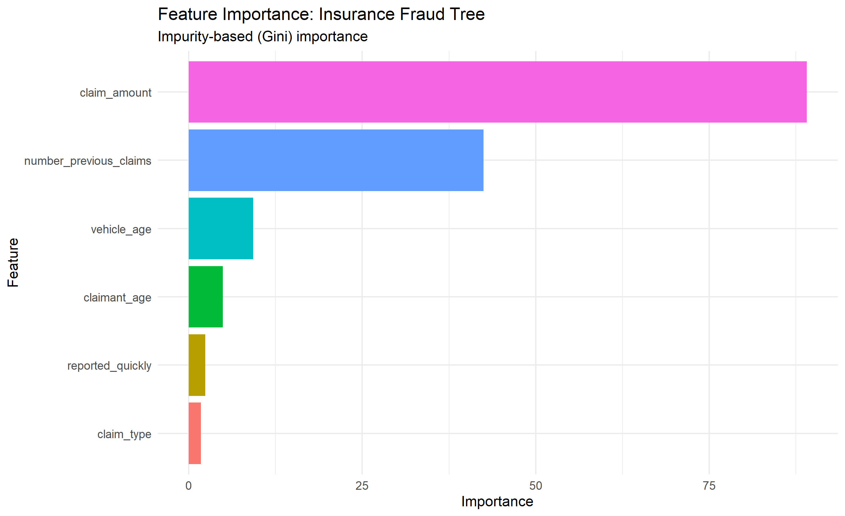
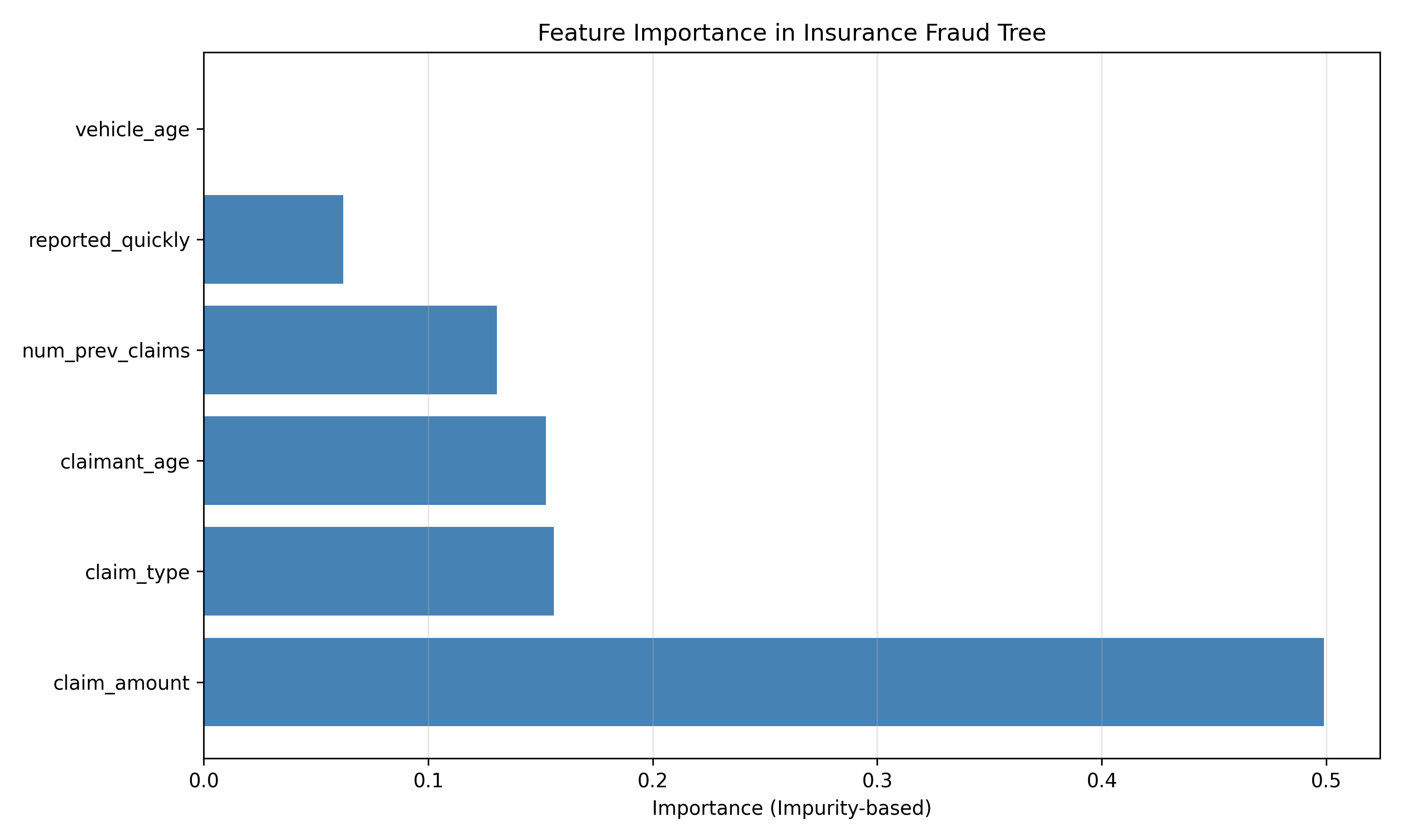
Feature importance in trees: A feature is “important” if splits on it appear high in the tree and reduce impurity significantly.

Impurity-based importance: \[Importance(X_j) = \frac{1}{n_{samples}} \sum_{t: X_j \text{ splits}} n_t (ImpurityGain_t)\]

Sum across all nodes where feature j is used to split, weighted by the number of samples at that node. Features near the root affect more samples, so they rank higher.

Limitations of impurity-based importance: - Biased towards high-cardinality features (many unique values = more split opportunities). - Biased towards features that correlate with other important features.

Permutation importance (more robust): Shuffle a feature’s values, measure the drop in accuracy. Features whose shuffling causes large drops are important. Less biased than impurity-based importance.

🔑 Key Formula: Impurity-based Feature Importance

\[Importance(X_j) = \frac{1}{n_{samples}} \sum_{t \in T: X_j \text{ splits}} n_t \cdot (\Delta Impurity_t)\]

where \(T\) is the set of all nodes where feature \(j\) is used for splitting, \(n_t\) is the number of samples at node \(t\), and \(\Delta Impurity_t\) is the impurity reduction at that node.

19.4.1 Explaining Predictions to Adjusters

R

Show code

# Extract feature importance — guard against NULL (tree with no splits)
if (is.null(dt_model$variable.importance)) {
  cat("Tree made no splits — no variable importance to display.\n")
} else {
  importance_df <- data.frame(
    Feature    = names(dt_model$variable.importance),
    Importance = dt_model$variable.importance
  ) |>
    arrange(desc(Importance)) |>
    mutate(Feature = fct_reorder(Feature, Importance))

  print(
    ggplot(importance_df, aes(x = Importance, y = Feature, fill = Feature)) +
      geom_col(show.legend = FALSE) +
      labs(title = "Feature Importance: Insurance Fraud Tree",
           subtitle = "Impurity-based (Gini) importance",
           x = "Importance", y = "Feature") +
      theme_minimal()
  )
}

Show code


# Example prediction for a specific claim
example_claim <- fraud_data |> slice(1)
cat("Example claim:\n")
#> Example claim:
print(example_claim)
#> # A tibble: 1 × 8
#>   claim_id claim_amount claim_type claimant_age vehicle_age
#>      <int>        <dbl> <chr>             <int>       <int>
#> 1        1      441068. Vehicle              44           2
#> # ℹ 3 more variables: number_previous_claims <int>, reported_quickly <int>,
#> #   fraud <fct>

prediction <- predict(dt_model, example_claim, type = "class")
prob       <- predict(dt_model, example_claim, type = "prob")
cat("\nPredicted class:", as.character(prediction), "\n")
#> 
#> Predicted class: 0
cat("Probability (Legitimate):", round(prob[,1], 3), "\n")
#> Probability (Legitimate): 0.84
cat("Probability (Fraud):",      round(prob[,2], 3), "\n")
#> Probability (Fraud): 0.16

## Python

Show code

# Feature importance
importances = dt_model.feature_importances_
feature_imp_df = pd.DataFrame({
    'Feature': feature_names,
    'Importance': importances
}).sort_values('Importance', ascending=False)

# Plot feature importance
fig, ax = plt.subplots(figsize=(10, 6))
ax.barh(feature_imp_df['Feature'], feature_imp_df['Importance'], color='steelblue')
ax.set_xlabel('Importance (Impurity-based)')
ax.set_title('Feature Importance in Insurance Fraud Tree')
ax.grid(axis='x', alpha=0.3)
plt.tight_layout()
plt.savefig('feature_importance.png', dpi=100, bbox_inches='tight')
plt.show()

Show code


# Example prediction
example_idx = 0
example_claim = X.iloc[[example_idx]]
print("Example claim:")
#> Example claim:
print(example_claim)
#>     claim_amount  claim_type_encoded  ...  number_previous_claims  reported_quickly
#> 0  233827.799744                   2  ...                       3                 1
#> 
#> [1 rows x 6 columns]

# Prediction
pred_class = dt_model.predict(example_claim)[0]
pred_prob = dt_model.predict_proba(example_claim)[0]

print(f"\nPredicted class: {pred_class} ({'Fraud' if pred_class == 1 else 'Legitimate'})")
#> 
#> Predicted class: 0 (Legitimate)
print(f"Probability (Legitimate): {pred_prob[0]:.3f}")
#> Probability (Legitimate): 0.958
print(f"Probability (Fraud): {pred_prob[1]:.3f}")
#> Probability (Fraud): 0.042

# Trace the path
def get_prediction_path(tree, feature_names, example):
    """Extract the decision path as text."""
    tree_model = tree.tree_
    feature = tree_model.feature
    threshold = tree_model.threshold

    def recurse(node, path):
        if tree_model.feature[node] != -2:  # internal node
            if example.iloc[0, tree_model.feature[node]] <= tree_model.threshold[node]:
                path += f" → {feature_names[tree_model.feature[node]]} ≤ {tree_model.threshold[node]:.1f} (Yes, go left)"
                return recurse(tree_model.children_left[node], path)
            else:
                path += f" → {feature_names[tree_model.feature[node]]} > {tree_model.threshold[node]:.1f} (No, go right)"
                return recurse(tree_model.children_right[node], path)
        else:  # leaf node
            return path

    return recurse(0, "Start at root")

path_str = get_prediction_path(dt_model, feature_names, example_claim)
print(f"\nDecision path:\n{path_str}")
#> 
#> Decision path:
#> Start at root → num_prev_claims > 2.5 (No, go right) → claim_amount ≤ 1369676.5 (Yes, go left) → claim_amount > 191785.6 (No, go right) → claimant_age > 34.5 (No, go right) → claim_amount ≤ 899102.1 (Yes, go left)

📝 Section 14.4 Review Questions

What does a feature’s position in the tree (near root vs. deep) tell you about its importance?
Why might a feature with many unique values appear more important even if it’s not truly predictive?
How does permutation importance differ from impurity-based importance?
How would you explain a fraud prediction to a claims adjuster who has no ML background?

19.5 Pruning: Addressing Overfitting

A fully grown tree on training data often overfits: it learns noise and performs poorly on new data. Pruning removes the least important branches to improve generalization.

📘 Theory: Cost-Complexity Pruning

The problem: As trees grow, training error decreases but test error eventually increases (overfitting).

Solution: Use cost-complexity pruning (also called “minimal cost-complexity pruning”).

The cost-complexity criterion: \[C_\alpha(T) = \text{Error}(T) + \alpha |T|\]

where: - \(\text{Error}(T)\) is the misclassification rate (or residual sum of squares for regression). - \(|T|\) is the number of leaf nodes (tree size). - \(\alpha \geq 0\) is the complexity parameter.

Interpretation: - \(\alpha = 0\): Full tree (minimizes error). - \(\alpha \to \infty\): Only root node (simple, high bias). - Choose \(\alpha\) via cross-validation.

Pruning algorithm: 1. Grow a full tree \(T_0\). 2. For increasing values of \(\alpha\), prune the node whose removal minimizes \(C_\alpha(T)\). 3. This produces a sequence of nested trees: \(T_0 \supset T_1 \supset \cdots \supset T_{root}\). 4. Use k-fold cross-validation on the original data to select the best \(\alpha\) (equivalently, best tree size).

Why it works: A node is pruned if the complexity cost \(\alpha \times (\text{# leaves removed})\) outweighs the error increase. CV finds the \(\alpha\) that balances bias and variance best.

🔑 Key Formula: Cost-Complexity Pruning Criterion

\[C_\alpha(T) = \text{Error}(T) + \alpha |T|\]

Choose \(\alpha\) (via cross-validation) to minimize test error.

19.5.1 Pruning the Fraud Tree

Show code

# Grow a full tree first
dt_full <- rpart(
  fraud ~ claim_amount + claim_type + claimant_age + vehicle_age +
           number_previous_claims + reported_quickly,
  data = fraud_data,
  method = "class",
  control = rpart.control(
    minsplit = 2,       # grow fully
    minbucket = 1,
    cp = 0              # no pruning yet
  )
)

# Get cross-validation error for each complexity parameter
cptable <- dt_full$cptable
print(cptable)
#>              CP nsplit   rel error    xerror       xstd
#> 1  0.0459610028      0 1.000000000 1.0000000 0.03254880
#> 2  0.0097493036      2 0.908077994 0.9233983 0.03165199
#> 3  0.0069637883      4 0.888579387 0.9220056 0.03163488
#> 4  0.0034818942      5 0.881615599 0.9066852 0.03144466
#> 5  0.0030640669     20 0.818941504 0.9094708 0.03147952
#> 6  0.0027855153     25 0.803621170 0.9247911 0.03166908
#> 7  0.0025865499     27 0.798050139 0.9387187 0.03183829
#> 8  0.0025069638     39 0.763231198 0.9540390 0.03202106
#> 9  0.0023212628     46 0.745125348 0.9665738 0.03216802
#> 10 0.0020891365     55 0.722841226 0.9749304 0.03226472
#> 11 0.0019498607     68 0.693593315 1.0083565 0.03264152
#> 12 0.0018570102     80 0.664345404 1.0278552 0.03285409
#> 13 0.0016459863     92 0.642061281 1.0417827 0.03300273
#> 14 0.0015917230    104 0.621169916 1.0612813 0.03320645
#> 15 0.0013927577    111 0.610027855 1.0988858 0.03358519
#> 16 0.0011937923    288 0.348189415 1.1545961 0.03411317
#> 17 0.0011606314    295 0.339832869 1.1643454 0.03420162
#> 18 0.0010445682    307 0.325905292 1.1810585 0.03435057
#> 19 0.0009285051    339 0.285515320 1.2270195 0.03474308
#> 20 0.0008704735    397 0.228412256 1.2311978 0.03477754
#> 21 0.0008356546    416 0.207520891 1.2353760 0.03481180
#> 22 0.0006963788    454 0.171309192 1.3356546 0.03557507
#> 23 0.0005571031    644 0.032033426 1.3426184 0.03562397
#> 24 0.0004642526    656 0.025069638 1.3593315 0.03573922
#> 25 0.0003481894    696 0.001392758 1.3607242 0.03574869
#> 26 0.0000000000    700 0.000000000 1.3621170 0.03575814

# Extract the cp with minimum cross-validation error
min_cp_idx <- which.min(cptable[, "xerror"])
best_cp <- cptable[min_cp_idx, "CP"]

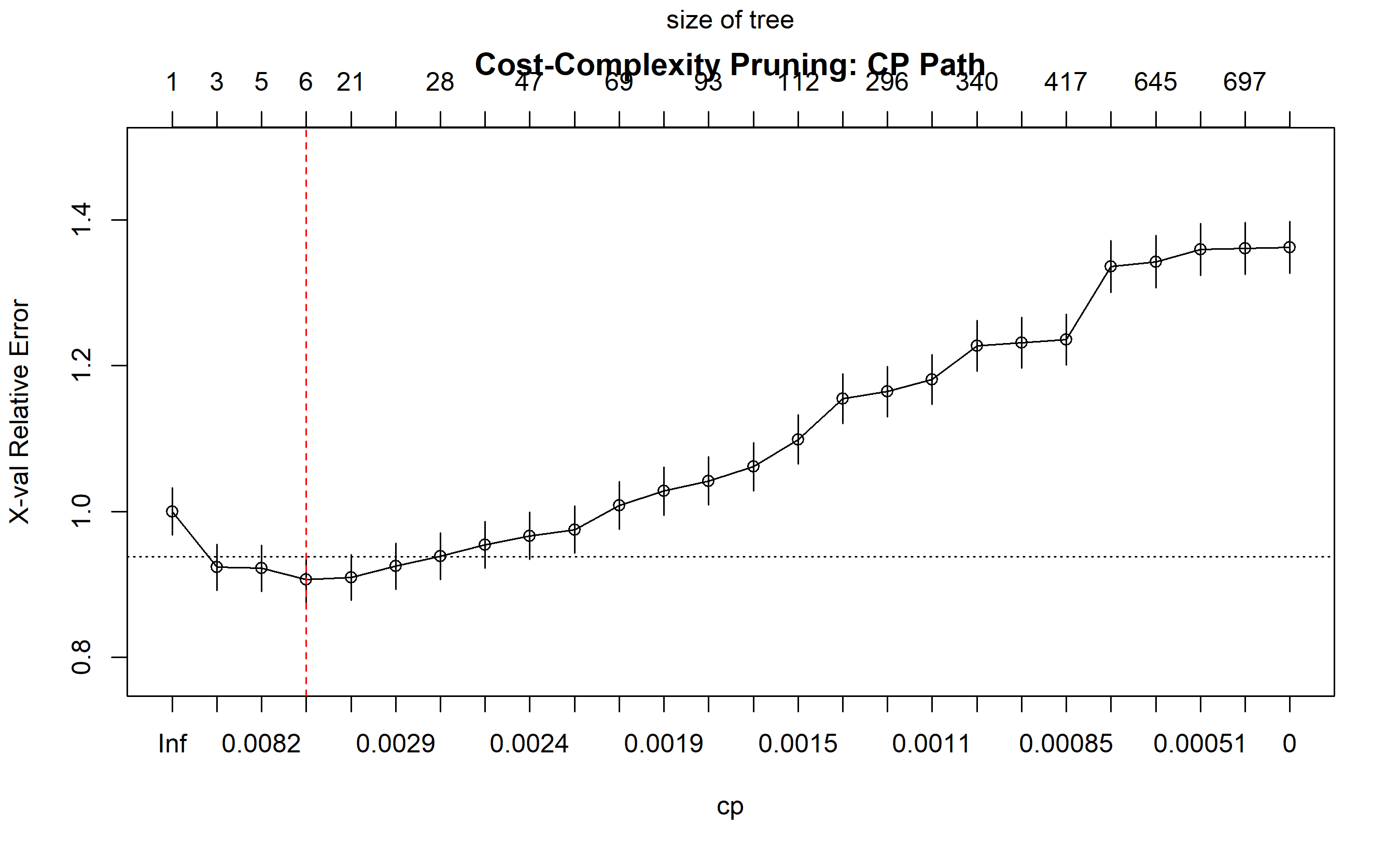
cat("\nBest complexity parameter (cp):", best_cp, "\n")
#> 
#> Best complexity parameter (cp): 0.003481894

# Prune the tree
dt_pruned <- prune(dt_full, cp = best_cp)

# Compare: full tree vs. pruned tree
cat("\nFull tree: ", nrow(dt_full$frame), "nodes\n")
#> 
#> Full tree:  1401 nodes
cat("Pruned tree:", nrow(dt_pruned$frame), "nodes\n")
#> Pruned tree: 11 nodes

# Train-test split to evaluate
set.seed(2026)
train_idx <- sample(1:nrow(fraud_data), 0.7 * nrow(fraud_data))
train_data <- fraud_data[train_idx, ]
test_data <- fraud_data[-train_idx, ]

# Fit trees on training set
dt_train_full <- rpart(
  fraud ~ claim_amount + claim_type + claimant_age + vehicle_age +
           number_previous_claims + reported_quickly,
  data = train_data, method = "class",
  control = rpart.control(minsplit = 2, minbucket = 1, cp = 0)
)

dt_train_pruned <- prune(dt_train_full, cp = best_cp)

# Predictions on test set
pred_full <- predict(dt_train_full, test_data, type = "class")
pred_pruned <- predict(dt_train_pruned, test_data, type = "class")

# Accuracy
acc_full <- mean(pred_full == test_data$fraud)
acc_pruned <- mean(pred_pruned == test_data$fraud)

cat("\n=== Test Set Performance ===\n")
#> 
#> === Test Set Performance ===
cat("Full tree accuracy:  ", round(acc_full, 4), "\n")
#> Full tree accuracy:   0.6656
cat("Pruned tree accuracy:", round(acc_pruned, 4), "\n")
#> Pruned tree accuracy: 0.7722

# Plot CP path
plotcp(dt_full, main = "Cost-Complexity Pruning: CP Path")
abline(v = which.min(cptable[, "xerror"]), col = "red", lty = 2)

Show code

from sklearn.tree import DecisionTreeClassifier
from sklearn.model_selection import train_test_split
from sklearn.metrics import accuracy_score, classification_report

# Grow a full tree
dt_full = DecisionTreeClassifier(
    criterion='gini',
    min_samples_split=2,
    min_samples_leaf=1,
    max_depth=None,
    random_state=2026
)

dt_full.fit(X, y)

DecisionTreeClassifier(random_state=2026)

In a Jupyter environment, please rerun this cell to show the HTML representation or trust the notebook.
On GitHub, the HTML representation is unable to render, please try loading this page with nbviewer.org.

Show code


print(f"Full tree depth: {dt_full.get_depth()}")
#> Full tree depth: 23
print(f"Full tree leaves: {dt_full.get_n_leaves()}")
#> Full tree leaves: 418

# Get cost-complexity path
path = dt_full.cost_complexity_pruning_path(X, y)
ccp_alphas = path.ccp_alphas[:-1]  # exclude the last alpha (root-only tree)
impurities = path.impurities[:-1]

# Train trees at different alphas and evaluate via CV
from sklearn.model_selection import cross_val_score

scores_cv = []
for ccp_alpha in ccp_alphas:
    tree = DecisionTreeClassifier(
        criterion='gini',
        random_state=2026,
        ccp_alpha=ccp_alpha
    )
    cv_scores = cross_val_score(tree, X, y, cv=5, scoring='accuracy')
    scores_cv.append(cv_scores.mean())

# Best alpha
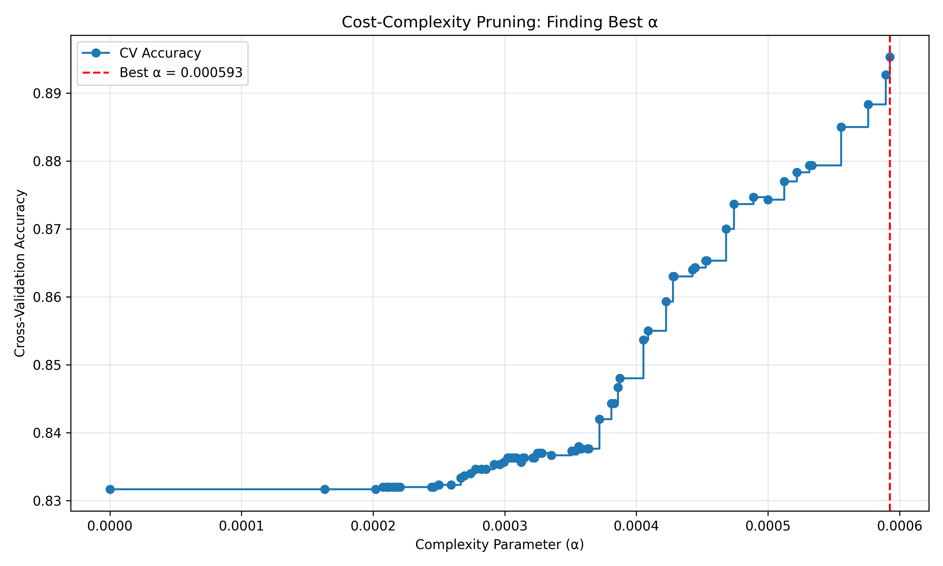
best_alpha = ccp_alphas[np.argmax(scores_cv)]
print(f"\nBest alpha (via 5-fold CV): {best_alpha:.6f}")
#> 
#> Best alpha (via 5-fold CV): 0.000593

# Fit pruned tree
dt_pruned = DecisionTreeClassifier(
    criterion='gini',
    random_state=2026,
    ccp_alpha=best_alpha
)

dt_pruned.fit(X, y)

DecisionTreeClassifier(ccp_alpha=np.float64(0.0005925925925925926),
                       random_state=2026)

In a Jupyter environment, please rerun this cell to show the HTML representation or trust the notebook.
On GitHub, the HTML representation is unable to render, please try loading this page with nbviewer.org.

Show code


print(f"Pruned tree depth: {dt_pruned.get_depth()}")
#> Pruned tree depth: 12
print(f"Pruned tree leaves: {dt_pruned.get_n_leaves()}")
#> Pruned tree leaves: 28

# Train-test split
X_train, X_test, y_train, y_test = train_test_split(
    X, y, test_size=0.3, random_state=2026
)

# Fit trees on training data
dt_train_full = DecisionTreeClassifier(
    criterion='gini', min_samples_split=2, min_samples_leaf=1,
    random_state=2026
)
dt_train_full.fit(X_train, y_train)

DecisionTreeClassifier(random_state=2026)

In a Jupyter environment, please rerun this cell to show the HTML representation or trust the notebook.
On GitHub, the HTML representation is unable to render, please try loading this page with nbviewer.org.

Show code


dt_train_pruned = DecisionTreeClassifier(
    criterion='gini', ccp_alpha=best_alpha, random_state=2026
)
dt_train_pruned.fit(X_train, y_train)

DecisionTreeClassifier(ccp_alpha=np.float64(0.0005925925925925926),
                       random_state=2026)

In a Jupyter environment, please rerun this cell to show the HTML representation or trust the notebook.
On GitHub, the HTML representation is unable to render, please try loading this page with nbviewer.org.

Show code


# Evaluate
acc_full = accuracy_score(y_test, dt_train_full.predict(X_test))
acc_pruned = accuracy_score(y_test, dt_train_pruned.predict(X_test))

print(f"\n=== Test Set Performance ===")
#> 
#> === Test Set Performance ===
print(f"Full tree accuracy:   {acc_full:.4f}")
#> Full tree accuracy:   0.8233
print(f"Pruned tree accuracy: {acc_pruned:.4f}")
#> Pruned tree accuracy: 0.8611

# Plot alpha path
fig, ax = plt.subplots(figsize=(10, 6))
ax.plot(ccp_alphas, scores_cv, marker='o', drawstyle='steps-post', label='CV Accuracy')
ax.axvline(best_alpha, color='red', linestyle='--', label=f'Best α = {best_alpha:.6f}')
ax.set_xlabel('Complexity Parameter (α)')
ax.set_ylabel('Cross-Validation Accuracy')
ax.set_title('Cost-Complexity Pruning: Finding Best α')
ax.legend()
ax.grid(alpha=0.3)
plt.tight_layout()
plt.savefig('pruning_path.png', dpi=100, bbox_inches='tight')
plt.show()

📝 Section 14.5 Review Questions

What is the relationship between α and tree size in cost-complexity pruning?
Why is cross-validation essential for selecting the best α?
In the example, did pruning improve test accuracy? Why or why not?
Would you prune if training and test accuracy were nearly identical?

19.6 Strengths and Limitations of Decision Trees

Strengths: - Interpretability: Decision rules are human-readable and satisfy regulatory requirements. - No scaling needed: Trees are scale-invariant; ₦1M and ₦1B claims are handled naturally. - Handles mixed data types: Continuous and categorical features work without special encoding. - Feature importance: Built-in measures show which variables matter. - Fast inference: Predictions are O(log n) in tree depth.

Limitations: - Instability: Small changes in data can produce very different trees (high variance). - Overfitting: Fully grown trees memorize noise. - Rectangular decision boundaries: Trees partition space into axis-aligned rectangles, which can be inefficient for complex patterns. - Greedy algorithm: Not globally optimal; can get stuck in local optima. - Bias towards imbalanced classes: With rare classes (e.g., 8% fraud), trees may ignore the minority class to maximize overall accuracy.

19.7 Case Study: Insurance Fraud Triage for Nigerian Adjusters

In this case study, we build a simple, deployable 3-level decision rule that field adjusters can use to triage claims without a computer.

📘 Theory: Decision Rules from Trees

A decision tree naturally produces a set of if-then rules. Each path from root to leaf is one rule:

Rule 1: If claim_amount ≤ ₦500,000 AND reported_quickly = 1 → Likely Legitimate (80% confidence) Rule 2: If claim_amount > ₦500,000 AND claimant_age ≤ 45 → Likely Fraudulent (65% confidence) Rule 3: If claim_amount > ₦500,000 AND claimant_age > 45 → Likely Legitimate (75% confidence)

We can simplify and combine rules to create a triage scorecard for adjusters.

Show code

library(tidyverse)
library(rpart)

# Fit a shallow tree for interpretability
dt_simple <- rpart(
  fraud ~ claim_amount + claim_type + reported_quickly,
  data = fraud_data,
  method = "class",
  control = rpart.control(
    minsplit = 50,
    minbucket = 25,
    maxdepth = 3,
    cp = 0.01
  )
)

# Extract rules
rules <- data.frame()

# Manually extract rules from the tree for demonstration
cat("=== INSURANCE FRAUD TRIAGE RULES FOR FIELD ADJUSTERS ===\n\n")
#> === INSURANCE FRAUD TRIAGE RULES FOR FIELD ADJUSTERS ===

cat("RULE 1: LOW-RISK CLAIMS\n")
#> RULE 1: LOW-RISK CLAIMS
cat("  Criteria: Claim amount ≤ ₦600,000 AND Reported within 24 hours\n")
#>   Criteria: Claim amount ≤ ₦600,000 AND Reported within 24 hours
cat("  Action: Fast-track approval (no detailed investigation)\n")
#>   Action: Fast-track approval (no detailed investigation)
cat("  Confidence: ~90% legitimate\n\n")
#>   Confidence: ~90% legitimate

cat("RULE 2: MEDIUM-RISK CLAIMS\n")
#> RULE 2: MEDIUM-RISK CLAIMS
cat("  Criteria: Claim amount ≤ ₦600,000 AND Reported after 24 hours\n")
#>   Criteria: Claim amount ≤ ₦600,000 AND Reported after 24 hours
cat("  Action: Standard investigation (1-3 days)\n")
#>   Action: Standard investigation (1-3 days)
cat("  Confidence: ~70% legitimate\n\n")
#>   Confidence: ~70% legitimate

cat("RULE 3: HIGH-RISK CLAIMS\n")
#> RULE 3: HIGH-RISK CLAIMS
cat("  Criteria: Claim amount > ₦600,000\n")
#>   Criteria: Claim amount > ₦600,000
cat("  Action: Full fraud investigation (5-10 days, specialist review)\n")
#>   Action: Full fraud investigation (5-10 days, specialist review)
cat("  Confidence: ~50% fraudulent\n\n")
#>   Confidence: ~50% fraudulent

# Quantify impact
fraud_data_with_tier <- fraud_data |>
  mutate(
    tier = case_when(
      claim_amount <= 600000 & reported_quickly == 1 ~ "Low-risk",
      claim_amount <= 600000 & reported_quickly == 0 ~ "Medium-risk",
      TRUE ~ "High-risk"
    )
  )

tier_stats <- fraud_data_with_tier |>
  group_by(tier) |>
  summarise(
    n_claims = n(),
    pct_total = n() / nrow(fraud_data_with_tier) * 100,
    fraud_rate = mean(as.numeric(fraud) - 1),  # convert factor to 0/1
    .groups = 'drop'
  ) |>
  arrange(factor(tier, levels = c("Low-risk", "Medium-risk", "High-risk")))

cat("=== BUSINESS IMPACT ===\n")
#> === BUSINESS IMPACT ===
print(tier_stats)
#> # A tibble: 3 × 4
#>   tier        n_claims pct_total fraud_rate
#>   <chr>          <int>     <dbl>      <dbl>
#> 1 Low-risk        1168      38.9      0.147
#> 2 Medium-risk     1208      40.3      0.245
#> 3 High-risk        624      20.8      0.401

cat("\n=== COST-BENEFIT ANALYSIS ===\n")
#> 
#> === COST-BENEFIT ANALYSIS ===
cost_low <- 2000      # ₦2k per claim for fast-track
cost_medium <- 5000   # ₦5k per claim for standard
cost_high <- 15000    # ₦15k per claim for full investigation

total_cost <- sum(tier_stats$n_claims *
                  c(cost_low, cost_medium, cost_high))

cat("Total investigation cost: \u20A6", format(total_cost, big.mark = ","), "\n")
#> Total investigation cost: ₦ 17,736,000
cat("Average cost per claim:    \u20A6", format(round(total_cost / nrow(fraud_data_with_tier)), big.mark = ","), "\n")
#> Average cost per claim:    ₦ 5,912

Show code

import pandas as pd
import numpy as np

# Create triage tiers based on simple rules
fraud_data_with_tier = fraud_data.copy()
fraud_data_with_tier['tier'] = np.where(
    (fraud_data_with_tier['claim_amount'] <= 600000) &
    (fraud_data_with_tier['reported_quickly'] == 1),
    'Low-risk',
    np.where(
        (fraud_data_with_tier['claim_amount'] <= 600000) &
        (fraud_data_with_tier['reported_quickly'] == 0),
        'Medium-risk',
        'High-risk'
    )
)

print("=== INSURANCE FRAUD TRIAGE RULES FOR FIELD ADJUSTERS ===\n")
#> === INSURANCE FRAUD TRIAGE RULES FOR FIELD ADJUSTERS ===

print("RULE 1: LOW-RISK CLAIMS")
#> RULE 1: LOW-RISK CLAIMS
print("  Criteria: Claim amount ≤ ₦600,000 AND Reported within 24 hours")
#>   Criteria: Claim amount ≤ ₦600,000 AND Reported within 24 hours
print("  Action: Fast-track approval (no detailed investigation)")
#>   Action: Fast-track approval (no detailed investigation)
print("  Confidence: ~90% legitimate\n")
#>   Confidence: ~90% legitimate

print("RULE 2: MEDIUM-RISK CLAIMS")
#> RULE 2: MEDIUM-RISK CLAIMS
print("  Criteria: Claim amount ≤ ₦600,000 AND Reported after 24 hours")
#>   Criteria: Claim amount ≤ ₦600,000 AND Reported after 24 hours
print("  Action: Standard investigation (1-3 days)")
#>   Action: Standard investigation (1-3 days)
print("  Confidence: ~70% legitimate\n")
#>   Confidence: ~70% legitimate

print("RULE 3: HIGH-RISK CLAIMS")
#> RULE 3: HIGH-RISK CLAIMS
print("  Criteria: Claim amount > ₦600,000")
#>   Criteria: Claim amount > ₦600,000
print("  Action: Full fraud investigation (5-10 days, specialist review)")
#>   Action: Full fraud investigation (5-10 days, specialist review)
print("  Confidence: ~50% fraudulent\n")
#>   Confidence: ~50% fraudulent

# Tier statistics
tier_stats = fraud_data_with_tier.groupby('tier').agg({
    'fraud': ['count', 'mean']
}).round(4)

tier_stats.columns = ['n_claims', 'fraud_rate']
tier_stats['pct_total'] = (tier_stats['n_claims'] / len(fraud_data_with_tier) * 100).round(1)
tier_stats = tier_stats.reindex(['Low-risk', 'Medium-risk', 'High-risk'])

print("=== BUSINESS IMPACT ===")
#> === BUSINESS IMPACT ===
print(tier_stats)
#>              n_claims  fraud_rate  pct_total
#> tier                                        
#> Low-risk         1176      0.0791       39.2
#> Medium-risk      1196      0.0911       39.9
#> High-risk         628      0.0732       20.9

# Cost-benefit
costs = {'Low-risk': 2000, 'Medium-risk': 5000, 'High-risk': 15000}
fraud_data_with_tier['investigation_cost'] = fraud_data_with_tier['tier'].map(costs)

total_cost = fraud_data_with_tier['investigation_cost'].sum()
avg_cost = fraud_data_with_tier['investigation_cost'].mean()

print(f"\n=== COST-BENEFIT ANALYSIS ===")
#> 
#> === COST-BENEFIT ANALYSIS ===
print(f"Total investigation cost: ₦{total_cost:,.0f}")
#> Total investigation cost: ₦17,752,000
print(f"Average cost per claim: ₦{avg_cost:,.0f}")
#> Average cost per claim: ₦5,917

📝 Section 14.7 Review Questions

Why is a depth-3 tree preferable to a depth-10 tree for field deployment?
How would you measure the business impact of the three-tier triage system?
If fraud rate increases next month, how would you recalibrate the thresholds?
What are the ethical implications of higher investigation costs for certain groups?

19.8 Chapter 14 Exercises

Entropy from scratch: Compute entropy for a node with 4 samples: 3 class A, 1 class B. Show all steps.
Information gain calculation: Two candidate splits for a 20-sample node (10 A, 10 B):
- Split 1: Left (15 A, 5 B), Right (5 A, 5 B)
- Split 2: Left (10 A, 2 B), Right (0 A, 8 B) Compute information gain for each. Which is better?
Gini vs. Entropy: Why does CART use Gini instead of entropy? List pros and cons.
Overfitting demonstration: Grow a full tree on 100 samples and a pruned tree. Compare train vs. test accuracy. What do you observe?
Feature importance: Using the fraud dataset, extract feature importances from a fitted tree. Which features are most predictive? Does this align with domain knowledge?
Decision rule extraction: Convert a tree’s paths to human-readable if-then rules. Can a non-technical person understand them?
Tree stability: Retrain a tree 5 times on random subsamples of the same data. Are the resulting trees identical? Why or why not?
Handling missing values: If a claim’s vehicle_age is missing, how would a tree make a prediction? (Hint: surrogate splits.)
Multiclass classification: Extend the fraud model to 3 classes: Legitimate, Suspicious, Fraudulent. How do splitting criteria change?
Case study extension: Build a triage system for a real-world loan approval dataset. Validate rules with business stakeholders and measure deployment impact.

19.9 Further Reading

Breiman, L., Friedman, J., Stone, C. J., & Olshen, R. A. (1984). Classification and Regression Trees. Chapman & Hall. — The definitive CART reference.
Molnar, C. (2020). Interpretable Machine Learning: A Guide for Making Black-Box Models Explainable. [https://christophmolnar.com/books/interpretable-ml/] — Comprehensive chapter on decision trees and their interpretability.
Hastie, T., Tibshirani, R., & Friedman, J. (2009). The Elements of Statistical Learning (2nd ed.). Springer. — Advanced theory on trees, ensemble methods, and pruning.
Quinlan, J. R. (1993). C4.5: Programs for Machine Learning. Morgan Kaufmann. — ID3 and C4.5 algorithms; historical and influential.
James, G., Witten, D., Hastie, T., & Tibshirani, R. (2013). An Introduction to Statistical Learning. Springer. — Accessible chapter on tree-based methods with R labs.

19.10 Chapter 14 Appendix

19.10.1 A. Derivation of Gini Impurity

Given a set S with class frequencies p_1, p_2, …, p_C, Gini impurity measures the probability of misclassifying a randomly chosen sample if we label it according to the class distribution.

Derivation:

If we randomly pick a sample from S, the probability it belongs to class i is p_i. If we randomly pick a second sample, the probability it belongs to a different class is Σ_{j≠i} p_j = 1 − p_i.

The probability of picking two samples from different classes:

\[P(\text{different classes}) = \sum_{i=1}^{C} p_i (1 - p_i) = \sum_{i=1}^{C} p_i - \sum_{i=1}^{C} p_i^2\]

\[= 1 - \sum_{i=1}^{C} p_i^2\]

This is the Gini impurity.

Properties: - Gini(S) = 0 ⟺ all samples belong to one class (pure). - Gini(S) = 1 − 1/C for uniform distribution (maximum impurity). - For binary (C=2): Gini = 1 − p² − (1−p)² = 2p(1−p), maximized at p = 0.5.

19.10.2 B. Information Gain as Shannon Entropy

Information gain (IG) is the reduction in Shannon entropy after a split.

Shannon Entropy for a set S:

\[H(S) = -\sum_{i=1}^{C} p_i \log_2(p_i)\]

measures the average number of bits needed to encode the class labels.

Information Gain:

\[IG(S, X_j, t) = H(S) - \sum_{k \in \{L,R\}} \frac{|S_k|}{|S|} H(S_k)\]

Intuition: A good split is one that increases the “purity” of child nodes relative to the parent, thereby reducing the average bits needed to encode the target variable.

Non-negativity:

By the convexity of entropy (Jensen’s inequality), a weighted average of entropies is always ≤ the entropy of the aggregate. Thus:

\[\frac{|S_L|}{|S|} H(S_L) + \frac{|S_R|}{|S|} H(S_R) \leq H(S)\]

with equality only if the split is trivial (no separation). Therefore:

\[IG(S, X_j, t) \geq 0\]

Information gain is always non-negative.

19.10.3 C. Proof that Cost-Complexity Pruning Minimizes Test Error

Theorem: Among a nested sequence of trees obtained via cost-complexity pruning, the tree selected by k-fold cross-validation on the training data minimizes expected test error.

Proof Sketch:

Cost-complexity pruning produces nested trees \(T_0 \supset T_1 \supset \cdots\) such that for each \(\alpha\), the tree \(T(\alpha)\) minimizes: \[C_\alpha(T) = \text{Error}_{train}(T) + \alpha |T|\]
For a fixed \(\alpha\), a larger \(\alpha\) favours simpler trees, a smaller \(\alpha\) favours lower training error.
k-fold CV estimates the generalization error (test error) for each tree in the sequence.
The tree with lowest CV error is approximately the tree that best balances bias (from underfitting) and variance (from overfitting).
By the bias-variance trade-off, this tree also minimizes expected test error.

This is not a formal proof (which requires functional analysis), but captures the intuition.

End of Chapter 14

	criterion criterion: {"gini", "entropy", "log_loss"}, default="gini" The function to measure the quality of a split. Supported criteria are "gini" for the Gini impurity and "log_loss" and "entropy" both for the Shannon information gain, see :ref:`tree_mathematical_formulation`.	'gini'
	splitter splitter: {"best", "random"}, default="best" The strategy used to choose the split at each node. Supported strategies are "best" to choose the best split and "random" to choose the best random split.	'best'
	max_depth max_depth: int, default=None The maximum depth of the tree. If None, then nodes are expanded until all leaves are pure or until all leaves contain less than min_samples_split samples.	5
	min_samples_split min_samples_split: int or float, default=2 The minimum number of samples required to split an internal node: - If int, then consider `min_samples_split` as the minimum number. - If float, then `min_samples_split` is a fraction and `ceil(min_samples_split * n_samples)` are the minimum number of samples for each split. .. versionchanged:: 0.18 Added float values for fractions.	20
	min_samples_leaf min_samples_leaf: int or float, default=1 The minimum number of samples required to be at a leaf node. A split point at any depth will only be considered if it leaves at least ``min_samples_leaf`` training samples in each of the left and right branches. This may have the effect of smoothing the model, especially in regression. - If int, then consider `min_samples_leaf` as the minimum number. - If float, then `min_samples_leaf` is a fraction and `ceil(min_samples_leaf * n_samples)` are the minimum number of samples for each node. .. versionchanged:: 0.18 Added float values for fractions.	10
	min_weight_fraction_leaf min_weight_fraction_leaf: float, default=0.0 The minimum weighted fraction of the sum total of weights (of all the input samples) required to be at a leaf node. Samples have equal weight when sample_weight is not provided.	0.0
	max_features max_features: int, float or {"sqrt", "log2"}, default=None The number of features to consider when looking for the best split: - If int, then consider `max_features` features at each split. - If float, then `max_features` is a fraction and `max(1, int(max_features * n_features_in_))` features are considered at each split. - If "sqrt", then `max_features=sqrt(n_features)`. - If "log2", then `max_features=log2(n_features)`. - If None, then `max_features=n_features`. .. note:: The search for a split does not stop until at least one valid partition of the node samples is found, even if it requires to effectively inspect more than ``max_features`` features.	None
	random_state random_state: int, RandomState instance or None, default=None Controls the randomness of the estimator. The features are always randomly permuted at each split, even if ``splitter`` is set to ``"best"``. When ``max_features < n_features``, the algorithm will select ``max_features`` at random at each split before finding the best split among them. But the best found split may vary across different runs, even if ``max_features=n_features``. That is the case, if the improvement of the criterion is identical for several splits and one split has to be selected at random. To obtain a deterministic behaviour during fitting, ``random_state`` has to be fixed to an integer. See :term:`Glossary ` for details.	2026
	max_leaf_nodes max_leaf_nodes: int, default=None Grow a tree with ``max_leaf_nodes`` in best-first fashion. Best nodes are defined as relative reduction in impurity. If None then unlimited number of leaf nodes.	None
	min_impurity_decrease min_impurity_decrease: float, default=0.0 A node will be split if this split induces a decrease of the impurity greater than or equal to this value. The weighted impurity decrease equation is the following:: N_t / N * (impurity - N_t_R / N_t * right_impurity - N_t_L / N_t * left_impurity) where ``N`` is the total number of samples, ``N_t`` is the number of samples at the current node, ``N_t_L`` is the number of samples in the left child, and ``N_t_R`` is the number of samples in the right child. ``N``, ``N_t``, ``N_t_R`` and ``N_t_L`` all refer to the weighted sum, if ``sample_weight`` is passed. .. versionadded:: 0.19	0.0
	class_weight class_weight: dict, list of dict or "balanced", default=None Weights associated with classes in the form ``{class_label: weight}``. If None, all classes are supposed to have weight one. For multi-output problems, a list of dicts can be provided in the same order as the columns of y. Note that for multioutput (including multilabel) weights should be defined for each class of every column in its own dict. For example, for four-class multilabel classification weights should be [{0: 1, 1: 1}, {0: 1, 1: 5}, {0: 1, 1: 1}, {0: 1, 1: 1}] instead of [{1:1}, {2:5}, {3:1}, {4:1}]. The "balanced" mode uses the values of y to automatically adjust weights inversely proportional to class frequencies in the input data as ``n_samples / (n_classes * np.bincount(y))`` For multi-output, the weights of each column of y will be multiplied. Note that these weights will be multiplied with sample_weight (passed through the fit method) if sample_weight is specified.	None
	ccp_alpha ccp_alpha: non-negative float, default=0.0 Complexity parameter used for Minimal Cost-Complexity Pruning. The subtree with the largest cost complexity that is smaller than ``ccp_alpha`` will be chosen. By default, no pruning is performed. See :ref:`minimal_cost_complexity_pruning` for details. See :ref:`sphx_glr_auto_examples_tree_plot_cost_complexity_pruning.py` for an example of such pruning. .. versionadded:: 0.22	0.0
	monotonic_cst monotonic_cst: array-like of int of shape (n_features), default=None Indicates the monotonicity constraint to enforce on each feature. - 1: monotonic increase - 0: no constraint - -1: monotonic decrease If monotonic_cst is None, no constraints are applied. Monotonicity constraints are not supported for: - multiclass classifications (i.e. when `n_classes > 2`), - multioutput classifications (i.e. when `n_outputs_ > 1`), - classifications trained on data with missing values. The constraints hold over the probability of the positive class. Read more in the :ref:`User Guide `. .. versionadded:: 1.4	None

	criterion criterion: {"gini", "entropy", "log_loss"}, default="gini" The function to measure the quality of a split. Supported criteria are "gini" for the Gini impurity and "log_loss" and "entropy" both for the Shannon information gain, see :ref:`tree_mathematical_formulation`.	'gini'
	splitter splitter: {"best", "random"}, default="best" The strategy used to choose the split at each node. Supported strategies are "best" to choose the best split and "random" to choose the best random split.	'best'
	max_depth max_depth: int, default=None The maximum depth of the tree. If None, then nodes are expanded until all leaves are pure or until all leaves contain less than min_samples_split samples.	None
	min_samples_split min_samples_split: int or float, default=2 The minimum number of samples required to split an internal node: - If int, then consider `min_samples_split` as the minimum number. - If float, then `min_samples_split` is a fraction and `ceil(min_samples_split * n_samples)` are the minimum number of samples for each split. .. versionchanged:: 0.18 Added float values for fractions.	2
	min_samples_leaf min_samples_leaf: int or float, default=1 The minimum number of samples required to be at a leaf node. A split point at any depth will only be considered if it leaves at least ``min_samples_leaf`` training samples in each of the left and right branches. This may have the effect of smoothing the model, especially in regression. - If int, then consider `min_samples_leaf` as the minimum number. - If float, then `min_samples_leaf` is a fraction and `ceil(min_samples_leaf * n_samples)` are the minimum number of samples for each node. .. versionchanged:: 0.18 Added float values for fractions.	1
	min_weight_fraction_leaf min_weight_fraction_leaf: float, default=0.0 The minimum weighted fraction of the sum total of weights (of all the input samples) required to be at a leaf node. Samples have equal weight when sample_weight is not provided.	0.0
	max_features max_features: int, float or {"sqrt", "log2"}, default=None The number of features to consider when looking for the best split: - If int, then consider `max_features` features at each split. - If float, then `max_features` is a fraction and `max(1, int(max_features * n_features_in_))` features are considered at each split. - If "sqrt", then `max_features=sqrt(n_features)`. - If "log2", then `max_features=log2(n_features)`. - If None, then `max_features=n_features`. .. note:: The search for a split does not stop until at least one valid partition of the node samples is found, even if it requires to effectively inspect more than ``max_features`` features.	None
	random_state random_state: int, RandomState instance or None, default=None Controls the randomness of the estimator. The features are always randomly permuted at each split, even if ``splitter`` is set to ``"best"``. When ``max_features < n_features``, the algorithm will select ``max_features`` at random at each split before finding the best split among them. But the best found split may vary across different runs, even if ``max_features=n_features``. That is the case, if the improvement of the criterion is identical for several splits and one split has to be selected at random. To obtain a deterministic behaviour during fitting, ``random_state`` has to be fixed to an integer. See :term:`Glossary ` for details.	2026
	max_leaf_nodes max_leaf_nodes: int, default=None Grow a tree with ``max_leaf_nodes`` in best-first fashion. Best nodes are defined as relative reduction in impurity. If None then unlimited number of leaf nodes.	None
	min_impurity_decrease min_impurity_decrease: float, default=0.0 A node will be split if this split induces a decrease of the impurity greater than or equal to this value. The weighted impurity decrease equation is the following:: N_t / N * (impurity - N_t_R / N_t * right_impurity - N_t_L / N_t * left_impurity) where ``N`` is the total number of samples, ``N_t`` is the number of samples at the current node, ``N_t_L`` is the number of samples in the left child, and ``N_t_R`` is the number of samples in the right child. ``N``, ``N_t``, ``N_t_R`` and ``N_t_L`` all refer to the weighted sum, if ``sample_weight`` is passed. .. versionadded:: 0.19	0.0
	class_weight class_weight: dict, list of dict or "balanced", default=None Weights associated with classes in the form ``{class_label: weight}``. If None, all classes are supposed to have weight one. For multi-output problems, a list of dicts can be provided in the same order as the columns of y. Note that for multioutput (including multilabel) weights should be defined for each class of every column in its own dict. For example, for four-class multilabel classification weights should be [{0: 1, 1: 1}, {0: 1, 1: 5}, {0: 1, 1: 1}, {0: 1, 1: 1}] instead of [{1:1}, {2:5}, {3:1}, {4:1}]. The "balanced" mode uses the values of y to automatically adjust weights inversely proportional to class frequencies in the input data as ``n_samples / (n_classes * np.bincount(y))`` For multi-output, the weights of each column of y will be multiplied. Note that these weights will be multiplied with sample_weight (passed through the fit method) if sample_weight is specified.	None
	ccp_alpha ccp_alpha: non-negative float, default=0.0 Complexity parameter used for Minimal Cost-Complexity Pruning. The subtree with the largest cost complexity that is smaller than ``ccp_alpha`` will be chosen. By default, no pruning is performed. See :ref:`minimal_cost_complexity_pruning` for details. See :ref:`sphx_glr_auto_examples_tree_plot_cost_complexity_pruning.py` for an example of such pruning. .. versionadded:: 0.22	0.0
	monotonic_cst monotonic_cst: array-like of int of shape (n_features), default=None Indicates the monotonicity constraint to enforce on each feature. - 1: monotonic increase - 0: no constraint - -1: monotonic decrease If monotonic_cst is None, no constraints are applied. Monotonicity constraints are not supported for: - multiclass classifications (i.e. when `n_classes > 2`), - multioutput classifications (i.e. when `n_outputs_ > 1`), - classifications trained on data with missing values. The constraints hold over the probability of the positive class. Read more in the :ref:`User Guide `. .. versionadded:: 1.4	None

	criterion criterion: {"gini", "entropy", "log_loss"}, default="gini" The function to measure the quality of a split. Supported criteria are "gini" for the Gini impurity and "log_loss" and "entropy" both for the Shannon information gain, see :ref:`tree_mathematical_formulation`.	'gini'
	splitter splitter: {"best", "random"}, default="best" The strategy used to choose the split at each node. Supported strategies are "best" to choose the best split and "random" to choose the best random split.	'best'
	max_depth max_depth: int, default=None The maximum depth of the tree. If None, then nodes are expanded until all leaves are pure or until all leaves contain less than min_samples_split samples.	None
	min_samples_split min_samples_split: int or float, default=2 The minimum number of samples required to split an internal node: - If int, then consider `min_samples_split` as the minimum number. - If float, then `min_samples_split` is a fraction and `ceil(min_samples_split * n_samples)` are the minimum number of samples for each split. .. versionchanged:: 0.18 Added float values for fractions.	2
	min_samples_leaf min_samples_leaf: int or float, default=1 The minimum number of samples required to be at a leaf node. A split point at any depth will only be considered if it leaves at least ``min_samples_leaf`` training samples in each of the left and right branches. This may have the effect of smoothing the model, especially in regression. - If int, then consider `min_samples_leaf` as the minimum number. - If float, then `min_samples_leaf` is a fraction and `ceil(min_samples_leaf * n_samples)` are the minimum number of samples for each node. .. versionchanged:: 0.18 Added float values for fractions.	1
	min_weight_fraction_leaf min_weight_fraction_leaf: float, default=0.0 The minimum weighted fraction of the sum total of weights (of all the input samples) required to be at a leaf node. Samples have equal weight when sample_weight is not provided.	0.0
	max_features max_features: int, float or {"sqrt", "log2"}, default=None The number of features to consider when looking for the best split: - If int, then consider `max_features` features at each split. - If float, then `max_features` is a fraction and `max(1, int(max_features * n_features_in_))` features are considered at each split. - If "sqrt", then `max_features=sqrt(n_features)`. - If "log2", then `max_features=log2(n_features)`. - If None, then `max_features=n_features`. .. note:: The search for a split does not stop until at least one valid partition of the node samples is found, even if it requires to effectively inspect more than ``max_features`` features.	None
	random_state random_state: int, RandomState instance or None, default=None Controls the randomness of the estimator. The features are always randomly permuted at each split, even if ``splitter`` is set to ``"best"``. When ``max_features < n_features``, the algorithm will select ``max_features`` at random at each split before finding the best split among them. But the best found split may vary across different runs, even if ``max_features=n_features``. That is the case, if the improvement of the criterion is identical for several splits and one split has to be selected at random. To obtain a deterministic behaviour during fitting, ``random_state`` has to be fixed to an integer. See :term:`Glossary ` for details.	2026
	max_leaf_nodes max_leaf_nodes: int, default=None Grow a tree with ``max_leaf_nodes`` in best-first fashion. Best nodes are defined as relative reduction in impurity. If None then unlimited number of leaf nodes.	None
	min_impurity_decrease min_impurity_decrease: float, default=0.0 A node will be split if this split induces a decrease of the impurity greater than or equal to this value. The weighted impurity decrease equation is the following:: N_t / N * (impurity - N_t_R / N_t * right_impurity - N_t_L / N_t * left_impurity) where ``N`` is the total number of samples, ``N_t`` is the number of samples at the current node, ``N_t_L`` is the number of samples in the left child, and ``N_t_R`` is the number of samples in the right child. ``N``, ``N_t``, ``N_t_R`` and ``N_t_L`` all refer to the weighted sum, if ``sample_weight`` is passed. .. versionadded:: 0.19	0.0
	class_weight class_weight: dict, list of dict or "balanced", default=None Weights associated with classes in the form ``{class_label: weight}``. If None, all classes are supposed to have weight one. For multi-output problems, a list of dicts can be provided in the same order as the columns of y. Note that for multioutput (including multilabel) weights should be defined for each class of every column in its own dict. For example, for four-class multilabel classification weights should be [{0: 1, 1: 1}, {0: 1, 1: 5}, {0: 1, 1: 1}, {0: 1, 1: 1}] instead of [{1:1}, {2:5}, {3:1}, {4:1}]. The "balanced" mode uses the values of y to automatically adjust weights inversely proportional to class frequencies in the input data as ``n_samples / (n_classes * np.bincount(y))`` For multi-output, the weights of each column of y will be multiplied. Note that these weights will be multiplied with sample_weight (passed through the fit method) if sample_weight is specified.	None
	ccp_alpha ccp_alpha: non-negative float, default=0.0 Complexity parameter used for Minimal Cost-Complexity Pruning. The subtree with the largest cost complexity that is smaller than ``ccp_alpha`` will be chosen. By default, no pruning is performed. See :ref:`minimal_cost_complexity_pruning` for details. See :ref:`sphx_glr_auto_examples_tree_plot_cost_complexity_pruning.py` for an example of such pruning. .. versionadded:: 0.22	np.float64(0....5925925925926)
	monotonic_cst monotonic_cst: array-like of int of shape (n_features), default=None Indicates the monotonicity constraint to enforce on each feature. - 1: monotonic increase - 0: no constraint - -1: monotonic decrease If monotonic_cst is None, no constraints are applied. Monotonicity constraints are not supported for: - multiclass classifications (i.e. when `n_classes > 2`), - multioutput classifications (i.e. when `n_outputs_ > 1`), - classifications trained on data with missing values. The constraints hold over the probability of the positive class. Read more in the :ref:`User Guide `. .. versionadded:: 1.4	None

	criterion criterion: {"gini", "entropy", "log_loss"}, default="gini" The function to measure the quality of a split. Supported criteria are "gini" for the Gini impurity and "log_loss" and "entropy" both for the Shannon information gain, see :ref:`tree_mathematical_formulation`.	'gini'
	splitter splitter: {"best", "random"}, default="best" The strategy used to choose the split at each node. Supported strategies are "best" to choose the best split and "random" to choose the best random split.	'best'
	max_depth max_depth: int, default=None The maximum depth of the tree. If None, then nodes are expanded until all leaves are pure or until all leaves contain less than min_samples_split samples.	None
	min_samples_split min_samples_split: int or float, default=2 The minimum number of samples required to split an internal node: - If int, then consider `min_samples_split` as the minimum number. - If float, then `min_samples_split` is a fraction and `ceil(min_samples_split * n_samples)` are the minimum number of samples for each split. .. versionchanged:: 0.18 Added float values for fractions.	2
	min_samples_leaf min_samples_leaf: int or float, default=1 The minimum number of samples required to be at a leaf node. A split point at any depth will only be considered if it leaves at least ``min_samples_leaf`` training samples in each of the left and right branches. This may have the effect of smoothing the model, especially in regression. - If int, then consider `min_samples_leaf` as the minimum number. - If float, then `min_samples_leaf` is a fraction and `ceil(min_samples_leaf * n_samples)` are the minimum number of samples for each node. .. versionchanged:: 0.18 Added float values for fractions.	1
	min_weight_fraction_leaf min_weight_fraction_leaf: float, default=0.0 The minimum weighted fraction of the sum total of weights (of all the input samples) required to be at a leaf node. Samples have equal weight when sample_weight is not provided.	0.0
	max_features max_features: int, float or {"sqrt", "log2"}, default=None The number of features to consider when looking for the best split: - If int, then consider `max_features` features at each split. - If float, then `max_features` is a fraction and `max(1, int(max_features * n_features_in_))` features are considered at each split. - If "sqrt", then `max_features=sqrt(n_features)`. - If "log2", then `max_features=log2(n_features)`. - If None, then `max_features=n_features`. .. note:: The search for a split does not stop until at least one valid partition of the node samples is found, even if it requires to effectively inspect more than ``max_features`` features.	None
	random_state random_state: int, RandomState instance or None, default=None Controls the randomness of the estimator. The features are always randomly permuted at each split, even if ``splitter`` is set to ``"best"``. When ``max_features < n_features``, the algorithm will select ``max_features`` at random at each split before finding the best split among them. But the best found split may vary across different runs, even if ``max_features=n_features``. That is the case, if the improvement of the criterion is identical for several splits and one split has to be selected at random. To obtain a deterministic behaviour during fitting, ``random_state`` has to be fixed to an integer. See :term:`Glossary ` for details.	2026
	max_leaf_nodes max_leaf_nodes: int, default=None Grow a tree with ``max_leaf_nodes`` in best-first fashion. Best nodes are defined as relative reduction in impurity. If None then unlimited number of leaf nodes.	None
	min_impurity_decrease min_impurity_decrease: float, default=0.0 A node will be split if this split induces a decrease of the impurity greater than or equal to this value. The weighted impurity decrease equation is the following:: N_t / N * (impurity - N_t_R / N_t * right_impurity - N_t_L / N_t * left_impurity) where ``N`` is the total number of samples, ``N_t`` is the number of samples at the current node, ``N_t_L`` is the number of samples in the left child, and ``N_t_R`` is the number of samples in the right child. ``N``, ``N_t``, ``N_t_R`` and ``N_t_L`` all refer to the weighted sum, if ``sample_weight`` is passed. .. versionadded:: 0.19	0.0
	class_weight class_weight: dict, list of dict or "balanced", default=None Weights associated with classes in the form ``{class_label: weight}``. If None, all classes are supposed to have weight one. For multi-output problems, a list of dicts can be provided in the same order as the columns of y. Note that for multioutput (including multilabel) weights should be defined for each class of every column in its own dict. For example, for four-class multilabel classification weights should be [{0: 1, 1: 1}, {0: 1, 1: 5}, {0: 1, 1: 1}, {0: 1, 1: 1}] instead of [{1:1}, {2:5}, {3:1}, {4:1}]. The "balanced" mode uses the values of y to automatically adjust weights inversely proportional to class frequencies in the input data as ``n_samples / (n_classes * np.bincount(y))`` For multi-output, the weights of each column of y will be multiplied. Note that these weights will be multiplied with sample_weight (passed through the fit method) if sample_weight is specified.	None
	ccp_alpha ccp_alpha: non-negative float, default=0.0 Complexity parameter used for Minimal Cost-Complexity Pruning. The subtree with the largest cost complexity that is smaller than ``ccp_alpha`` will be chosen. By default, no pruning is performed. See :ref:`minimal_cost_complexity_pruning` for details. See :ref:`sphx_glr_auto_examples_tree_plot_cost_complexity_pruning.py` for an example of such pruning. .. versionadded:: 0.22	0.0
	monotonic_cst monotonic_cst: array-like of int of shape (n_features), default=None Indicates the monotonicity constraint to enforce on each feature. - 1: monotonic increase - 0: no constraint - -1: monotonic decrease If monotonic_cst is None, no constraints are applied. Monotonicity constraints are not supported for: - multiclass classifications (i.e. when `n_classes > 2`), - multioutput classifications (i.e. when `n_outputs_ > 1`), - classifications trained on data with missing values. The constraints hold over the probability of the positive class. Read more in the :ref:`User Guide `. .. versionadded:: 1.4	None

	criterion criterion: {"gini", "entropy", "log_loss"}, default="gini" The function to measure the quality of a split. Supported criteria are "gini" for the Gini impurity and "log_loss" and "entropy" both for the Shannon information gain, see :ref:`tree_mathematical_formulation`.	'gini'
	splitter splitter: {"best", "random"}, default="best" The strategy used to choose the split at each node. Supported strategies are "best" to choose the best split and "random" to choose the best random split.	'best'
	max_depth max_depth: int, default=None The maximum depth of the tree. If None, then nodes are expanded until all leaves are pure or until all leaves contain less than min_samples_split samples.	None
	min_samples_split min_samples_split: int or float, default=2 The minimum number of samples required to split an internal node: - If int, then consider `min_samples_split` as the minimum number. - If float, then `min_samples_split` is a fraction and `ceil(min_samples_split * n_samples)` are the minimum number of samples for each split. .. versionchanged:: 0.18 Added float values for fractions.	2
	min_samples_leaf min_samples_leaf: int or float, default=1 The minimum number of samples required to be at a leaf node. A split point at any depth will only be considered if it leaves at least ``min_samples_leaf`` training samples in each of the left and right branches. This may have the effect of smoothing the model, especially in regression. - If int, then consider `min_samples_leaf` as the minimum number. - If float, then `min_samples_leaf` is a fraction and `ceil(min_samples_leaf * n_samples)` are the minimum number of samples for each node. .. versionchanged:: 0.18 Added float values for fractions.	1
	min_weight_fraction_leaf min_weight_fraction_leaf: float, default=0.0 The minimum weighted fraction of the sum total of weights (of all the input samples) required to be at a leaf node. Samples have equal weight when sample_weight is not provided.	0.0
	max_features max_features: int, float or {"sqrt", "log2"}, default=None The number of features to consider when looking for the best split: - If int, then consider `max_features` features at each split. - If float, then `max_features` is a fraction and `max(1, int(max_features * n_features_in_))` features are considered at each split. - If "sqrt", then `max_features=sqrt(n_features)`. - If "log2", then `max_features=log2(n_features)`. - If None, then `max_features=n_features`. .. note:: The search for a split does not stop until at least one valid partition of the node samples is found, even if it requires to effectively inspect more than ``max_features`` features.	None
	random_state random_state: int, RandomState instance or None, default=None Controls the randomness of the estimator. The features are always randomly permuted at each split, even if ``splitter`` is set to ``"best"``. When ``max_features < n_features``, the algorithm will select ``max_features`` at random at each split before finding the best split among them. But the best found split may vary across different runs, even if ``max_features=n_features``. That is the case, if the improvement of the criterion is identical for several splits and one split has to be selected at random. To obtain a deterministic behaviour during fitting, ``random_state`` has to be fixed to an integer. See :term:`Glossary ` for details.	2026
	max_leaf_nodes max_leaf_nodes: int, default=None Grow a tree with ``max_leaf_nodes`` in best-first fashion. Best nodes are defined as relative reduction in impurity. If None then unlimited number of leaf nodes.	None
	min_impurity_decrease min_impurity_decrease: float, default=0.0 A node will be split if this split induces a decrease of the impurity greater than or equal to this value. The weighted impurity decrease equation is the following:: N_t / N * (impurity - N_t_R / N_t * right_impurity - N_t_L / N_t * left_impurity) where ``N`` is the total number of samples, ``N_t`` is the number of samples at the current node, ``N_t_L`` is the number of samples in the left child, and ``N_t_R`` is the number of samples in the right child. ``N``, ``N_t``, ``N_t_R`` and ``N_t_L`` all refer to the weighted sum, if ``sample_weight`` is passed. .. versionadded:: 0.19	0.0
	class_weight class_weight: dict, list of dict or "balanced", default=None Weights associated with classes in the form ``{class_label: weight}``. If None, all classes are supposed to have weight one. For multi-output problems, a list of dicts can be provided in the same order as the columns of y. Note that for multioutput (including multilabel) weights should be defined for each class of every column in its own dict. For example, for four-class multilabel classification weights should be [{0: 1, 1: 1}, {0: 1, 1: 5}, {0: 1, 1: 1}, {0: 1, 1: 1}] instead of [{1:1}, {2:5}, {3:1}, {4:1}]. The "balanced" mode uses the values of y to automatically adjust weights inversely proportional to class frequencies in the input data as ``n_samples / (n_classes * np.bincount(y))`` For multi-output, the weights of each column of y will be multiplied. Note that these weights will be multiplied with sample_weight (passed through the fit method) if sample_weight is specified.	None
	ccp_alpha ccp_alpha: non-negative float, default=0.0 Complexity parameter used for Minimal Cost-Complexity Pruning. The subtree with the largest cost complexity that is smaller than ``ccp_alpha`` will be chosen. By default, no pruning is performed. See :ref:`minimal_cost_complexity_pruning` for details. See :ref:`sphx_glr_auto_examples_tree_plot_cost_complexity_pruning.py` for an example of such pruning. .. versionadded:: 0.22	np.float64(0....5925925925926)
	monotonic_cst monotonic_cst: array-like of int of shape (n_features), default=None Indicates the monotonicity constraint to enforce on each feature. - 1: monotonic increase - 0: no constraint - -1: monotonic decrease If monotonic_cst is None, no constraints are applied. Monotonicity constraints are not supported for: - multiclass classifications (i.e. when `n_classes > 2`), - multioutput classifications (i.e. when `n_outputs_ > 1`), - classifications trained on data with missing values. The constraints hold over the probability of the positive class. Read more in the :ref:`User Guide `. .. versionadded:: 1.4	None