---
title: "A/B Testing and Business Experimentation"
---
```{python}
#| label: python-setup-07
#| include: false
import numpy as np
import pandas as pd
import matplotlib.pyplot as plt
import seaborn as sns
from scipy.stats import norm, binom, beta as beta_dist
```
::: {.callout-note icon="false"}
## 📋 Learning Objectives
By the end of this chapter, you will be able to:
- Understand the fundamental logic of randomized controlled trials and the counterfactual problem they solve
- Design an A/B test: choose metrics, calculate minimum detectable effect, determine sample size, set test duration
- Apply frequentist hypothesis testing to A/B tests using the two-proportion z-test
- Interpret stopping rules and understand the peeking problem
- Understand Bayesian A/B testing from first principles: priors, likelihood, posteriors, and probability of being best
- Compare frequentist and Bayesian approaches and choose appropriately
- Understand multi-armed bandits: the explore-exploit trade-off and Thompson Sampling
- Identify and avoid common pitfalls: p-hacking, network effects, Simpson's paradox, survivorship bias
- Design and analyze a business experiment end-to-end in a real-world context
:::
## What Is a Business Experiment?
An experiment is different from observation. When you observe that users who have electricity access spend more on education, you've found a correlation—but does electricity cause higher spending, or do wealthier households both have electricity and can afford education? This is the **counterfactual problem**: you'll never know what would have happened had the user *not* received electricity. Randomized experiments solve this by creating two identical groups, treating one, and comparing outcomes.
::: {.callout-note icon="false"}
## 📘 Theory: Randomized Controlled Trials and Causal Inference
A **Randomized Controlled Trial (RCT)** is the gold standard for causal inference. You randomly assign subjects into treatment (experiences the intervention) and control (baseline) groups. Random assignment ensures the groups are balanced on all observed and unobserved characteristics on average. Any difference in outcomes between groups is attributable to the treatment, not to pre-existing differences.
Example: A West African fintech wants to know if a simplified onboarding flow increases conversion to active customers. They randomly assign 50% of new signups to the current flow (control) and 50% to a new, streamlined flow (treatment). After 30 days, they compare the proportion who completed onboarding. Because assignment was random, any difference is due to the flow change, not user differences.
**Internal vs. External Validity**:
- **Internal validity**: Did the experiment truly measure the causal effect? (Are results due to the treatment or confounds?)
- **External validity**: Do results generalize beyond the experiment? (Would the effect hold in other contexts?)
An experiment can have high internal validity (strong causal evidence) but low external validity (results don't generalize). A fintech's onboarding test might show a 5% lift when conducted on weekday mornings in Lagos, but the effect might be smaller on weekends or in rural areas.
**Why "Before-After" Comparisons Mislead**: Suppose you measure user satisfaction before a product change and again after. Satisfaction increased from 6/10 to 7/10. Did the change cause this? Not necessarily. Seasonal factors, regression to the mean, or simply users getting used to the interface could explain the improvement. Without a control group that didn't receive the change, you can't tell.
:::
::: {.callout-caution icon="false"}
## 📝 Section 7.1 Review Questions
1. Explain the counterfactual problem and how randomization solves it.
2. What is the difference between internal and external validity? Give an example.
3. Why is a before-after comparison insufficient to claim causality?
4. In a fintech context, describe how you would randomly assign users to treatment and control groups.
5. What could cause an experiment to have high internal validity but low external validity?
:::
## Designing an A/B Test
Designing an A/B test well is as important as analyzing it. Poor design leads to wasted time and inconclusive results.
::: {.callout-note icon="false"}
## 📘 Theory: Metrics, Effect Size, and Sample Size
**Choose Your Primary Metric**: What outcome matters? For an onboarding flow, is it conversion (completed onboarding), time to completion, or retention after 30 days? Different metrics have different variances and effect sizes. A high-variance metric (e.g., total spending, which varies widely) requires larger samples than a low-variance metric (e.g., binary conversion, 0 or 1).
**Specify Minimum Detectable Effect (MDE)**: How small an effect is worth detecting? If your hypothesis is that the new flow increases conversion from 40% to 45%, the effect size is 5 percentage points. Smaller effects require larger samples. An MDE should be set *a priori*, not chosen after seeing the data.
**Calculate Sample Size**: The formula depends on the test type. For a two-proportion test (comparing conversion rates):
$$n = 2 \left( z_{\alpha/2} + z_{\beta} \right)^2 \frac{p(1-p)}{(\Delta p)^2}$$
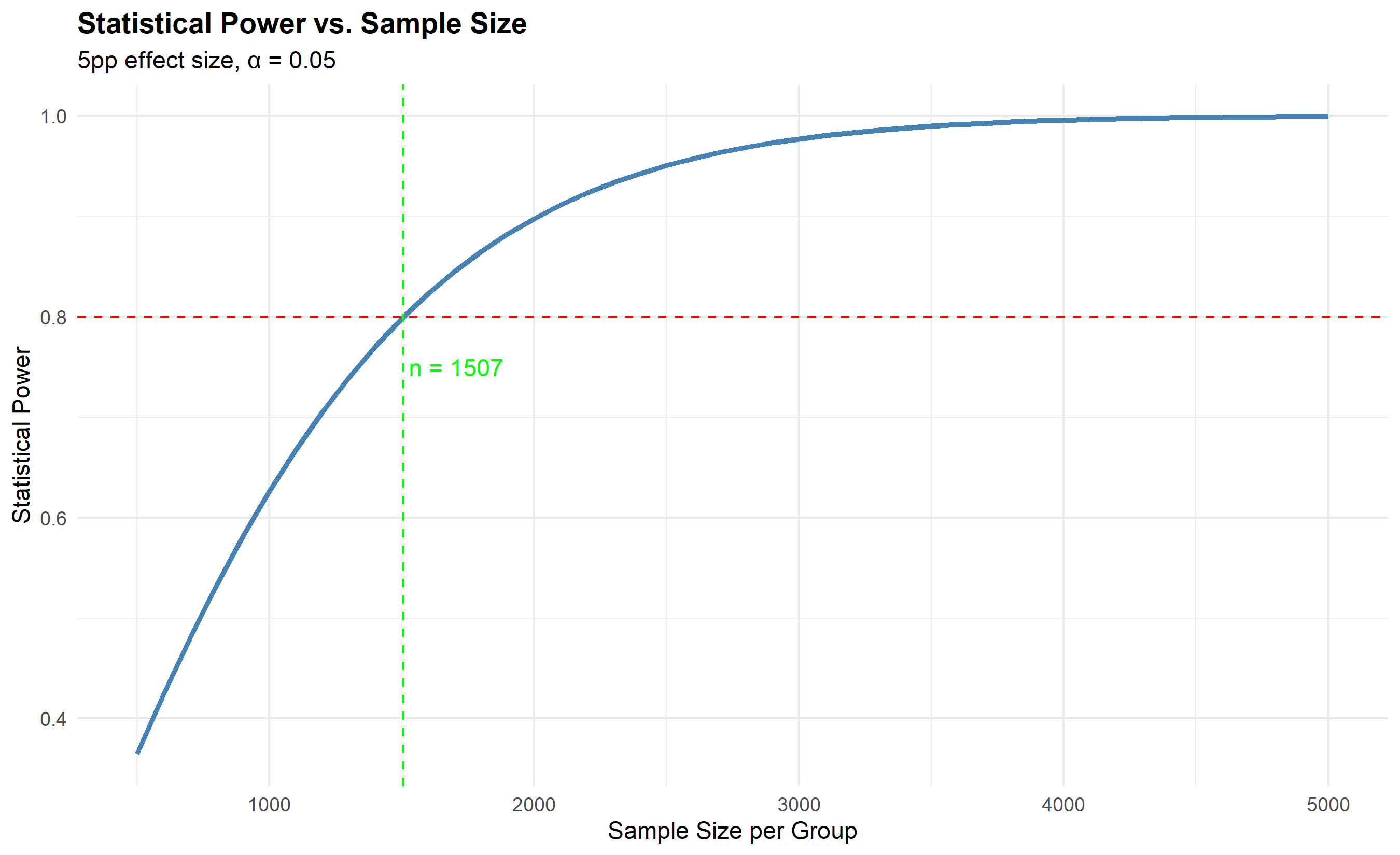
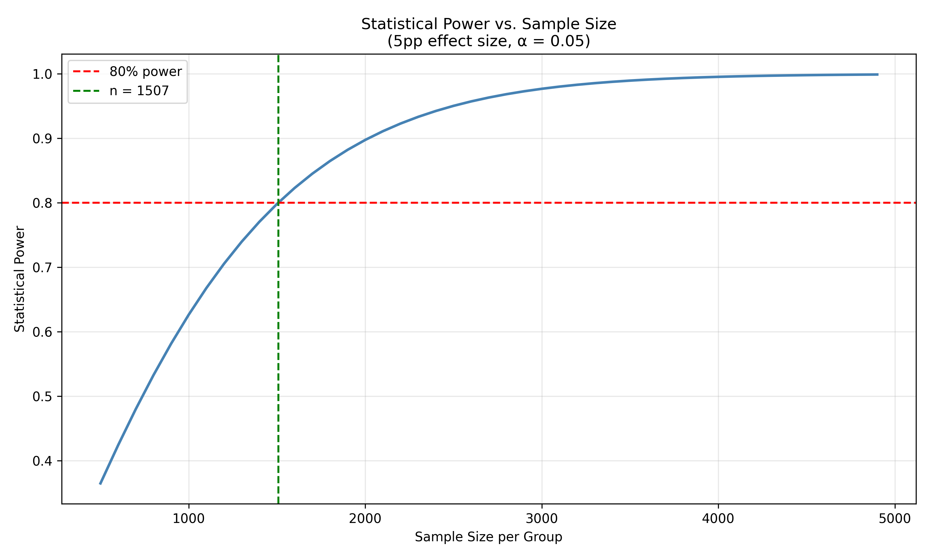
where p is the baseline conversion rate, Δp is the MDE, z_α/2 is the critical value for your significance level (typically 1.96 for α = 0.05), and z_β is the critical value for power (typically 0.84 for 80% power). The result is the sample size *per group*. With 80% power and 5% significance, if baseline conversion is 40% and MDE is 5 percentage points, you'd need roughly 1,000 users per group (2,000 total).
**Test Duration**: How long do you run the test? This depends on traffic and sample size. If you have 100 new signups per day and need 2,000 users, the test takes 20 days. Longer tests can detect seasonal or novelty effects, but patience has costs—delaying product changes means delayed value.
**Randomization**: How do you randomly assign? For web products, random number generation (each user gets a random number; even numbers = control, odd = treatment) is standard. Ensure randomization is reproducible and blinded: users shouldn't know which group they're in.
**Holdout Groups**: Always maintain a long-term holdout—a small percentage of users never exposed to the treatment, to measure long-term effects and detect if the treatment causes harm.
:::
::: {.callout-tip icon="false"}
## 🔑 Key Formula
**Sample Size for Two-Proportion Test:**
$$n = 2 \left( z_{\alpha/2} + z_{\beta} \right)^2 \frac{p(1-p)}{(\Delta p)^2}$$
**Effect Size (Cohen's h):**
$$h = 2 \arcsin(\sqrt{p_1}) - 2 \arcsin(\sqrt{p_2})$$
where p₁ and p₂ are the two proportions. Small effect: h ≈ 0.2, medium: h ≈ 0.5, large: h ≈ 0.8.
:::
::: {.panel-tabset}
## R
```{r}
library(tidyverse)
# Sample size calculation for A/B test
# Onboarding test: convert 40% (control) to 45% (treatment)
baseline_conversion <- 0.40
target_conversion <- 0.45
effect_size <- target_conversion - baseline_conversion
# Significance level and power
alpha <- 0.05
beta <- 0.20 # 80% power
z_alpha <- qnorm(1 - alpha / 2) # Two-tailed
z_beta <- qnorm(1 - beta)
# Sample size per group
p <- baseline_conversion
n_per_group <- 2 * ((z_alpha + z_beta)^2) * (p * (1 - p)) / effect_size^2
cat("=== A/B TEST DESIGN ===\n")
cat(sprintf("Baseline conversion rate: %.1f%%\n", baseline_conversion * 100))
cat(sprintf("Target conversion rate: %.1f%%\n", target_conversion * 100))
cat(sprintf("Minimum detectable effect: %.1f pp\n", effect_size * 100))
cat(sprintf("Significance level (α): %.3f\n", alpha))
cat(sprintf("Statistical power: %.1f%%\n", (1 - beta) * 100))
cat(sprintf("\nSample size per group: %.0f\n", n_per_group))
cat(sprintf("Total sample size: %.0f\n", 2 * n_per_group))
cat(sprintf("Test duration (at 100 users/day): %.0f days\n", 2 * n_per_group / 100))
# Power curve: How power changes with sample size
sample_sizes <- seq(500, 5000, by = 100)
powers <- sapply(sample_sizes, function(n) {
se <- sqrt(2 * p * (1 - p) / n)
z_critical <- qnorm(1 - alpha / 2)
power <- 1 - pnorm(z_critical - effect_size / se)
power
})
power_df <- tibble(
sample_per_group = sample_sizes,
power = powers
)
ggplot(power_df, aes(x = sample_per_group, y = power)) +
geom_line(linewidth = 1.2, color = "steelblue") +
geom_hline(yintercept = 0.80, linetype = "dashed", color = "red") +
geom_vline(xintercept = n_per_group, linetype = "dashed", color = "green") +
annotate("text", x = n_per_group + 200, y = 0.75,
label = sprintf("n = %.0f", n_per_group), color = "green") +
labs(
title = "Statistical Power vs. Sample Size",
x = "Sample Size per Group",
y = "Statistical Power",
subtitle = sprintf("5pp effect size, α = 0.05")
) +
theme_minimal() +
theme(plot.title = element_text(face = "bold"))
```
## Python
```{python}
import numpy as np
from scipy.stats import norm
import matplotlib.pyplot as plt
# Sample size calculation
baseline_conversion = 0.40
target_conversion = 0.45
effect_size = target_conversion - baseline_conversion
alpha = 0.05
beta = 0.20
z_alpha = norm.ppf(1 - alpha / 2)
z_beta = norm.ppf(1 - beta)
p = baseline_conversion
n_per_group = 2 * ((z_alpha + z_beta)**2) * (p * (1 - p)) / (effect_size**2)
print("=== A/B TEST DESIGN ===")
print(f"Baseline conversion rate: {baseline_conversion*100:.1f}%")
print(f"Target conversion rate: {target_conversion*100:.1f}%")
print(f"Minimum detectable effect: {effect_size*100:.1f} pp")
print(f"Significance level (α): {alpha:.3f}")
print(f"Statistical power: {(1-beta)*100:.1f}%")
print(f"\nSample size per group: {n_per_group:.0f}")
print(f"Total sample size: {2*n_per_group:.0f}")
print(f"Test duration (at 100 users/day): {2*n_per_group/100:.0f} days")
# Power curve
sample_sizes = np.arange(500, 5000, 100)
powers = []
for n in sample_sizes:
se = np.sqrt(2 * p * (1 - p) / n)
z_critical = norm.ppf(1 - alpha / 2)
power = 1 - norm.cdf(z_critical - effect_size / se)
powers.append(power)
# Plot
plt.figure(figsize=(10, 6))
plt.plot(sample_sizes, powers, linewidth=2, color='steelblue')
plt.axhline(0.80, linestyle='--', color='red', label='80% power')
plt.axvline(n_per_group, linestyle='--', color='green', label=f'n = {n_per_group:.0f}')
plt.xlabel('Sample Size per Group')
plt.ylabel('Statistical Power')
plt.title('Statistical Power vs. Sample Size\n(5pp effect size, α = 0.05)')
plt.legend()
plt.grid(alpha=0.3)
plt.tight_layout()
plt.show()
```
:::
::: {.callout-caution icon="false"}
## 📝 Section 7.2 Review Questions
1. What is the minimum detectable effect (MDE), and why should it be specified before the test?
2. How does baseline conversion rate affect required sample size?
3. What is the trade-off between test duration and sample size?
4. Why is random assignment critical to A/B tests?
5. How would you maintain a control group long-term to detect delayed effects?
:::
## Frequentist A/B Testing
The frequentist approach uses the two-proportion z-test: you compare the conversion rate in treatment to the conversion rate in control and compute a p-value.
::: {.callout-note icon="false"}
## 📘 Theory: The Two-Proportion Z-Test
After the test runs, you observe:
- Control: x₀ conversions out of n₀ users, conversion rate p₀ = x₀ / n₀
- Treatment: x₁ conversions out of n₁ users, conversion rate p₁ = x₁ / n₁
The test statistic is:
$$z = \frac{p_1 - p_0}{\sqrt{p(1-p) \left( \frac{1}{n_0} + \frac{1}{n_1} \right)}}$$
where $p = \frac{x_0 + x_1}{n_0 + n_1}$ is the pooled conversion rate. Under the null (no difference), z follows a standard normal distribution. You compute a two-tailed p-value and compare to α = 0.05. If p < 0.05, reject the null and declare the treatment superior (or inferior if the effect is in the opposite direction).
**One-Sided vs. Two-Sided**: A one-sided test asks "Is the treatment *better* than control?" A two-sided test asks "Is there *any* difference?" Most A/B tests should be two-sided unless you have a strong *a priori* reason to expect only positive effects.
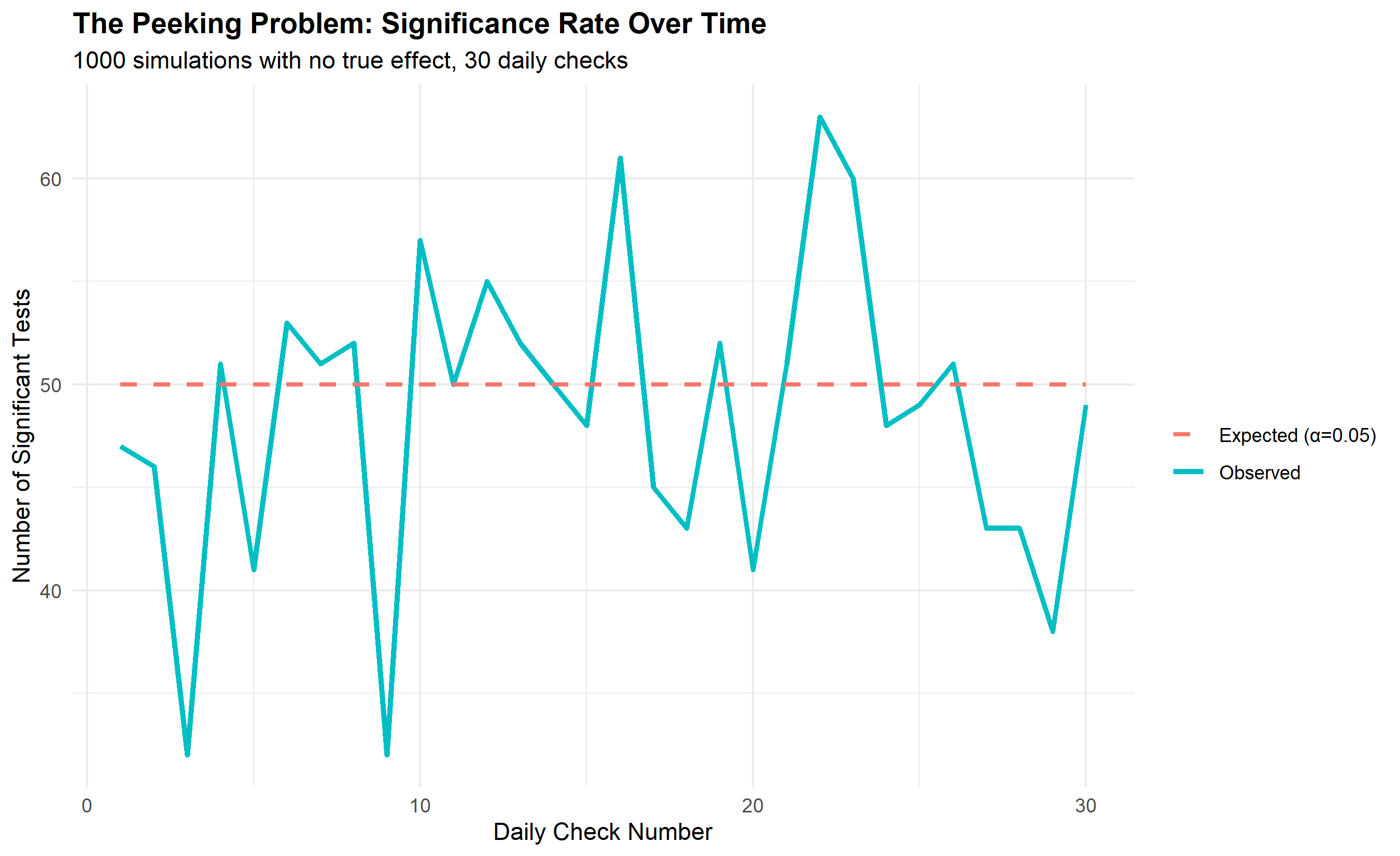
**The Peeking Problem**: Suppose you decide to check results every day. Each check is a hypothesis test, and if you run 30 checks at α = 0.05, the false positive rate across all checks inflates to ~78% (not 5%). This is *optional stopping* or *peeking*. The solution: commit to a sample size and significance level *before* peeking, or use a sequential testing approach (spending function, alpha-spending).
:::
Let's simulate and analyze a frequentist A/B test:
::: {.panel-tabset}
## R
```{r}
library(binom)
# Simulate A/B test results
set.seed(123)
# True conversion rates
p_control <- 0.40
p_treatment <- 0.45 # 5pp lift
# Sample sizes (from design)
n_per_group <- 1000
# Simulate data
conversions_control <- rbinom(1, n_per_group, p_control)
conversions_treatment <- rbinom(1, n_per_group, p_treatment)
cat("=== A/B TEST RESULTS ===\n")
cat(sprintf("Control: %d / %d = %.2f%%\n",
conversions_control, n_per_group,
100 * conversions_control / n_per_group))
cat(sprintf("Treatment: %d / %d = %.2f%%\n",
conversions_treatment, n_per_group,
100 * conversions_treatment / n_per_group))
# Two-proportion z-test
p0 <- conversions_control / n_per_group
p1 <- conversions_treatment / n_per_group
p_pooled <- (conversions_control + conversions_treatment) / (2 * n_per_group)
se <- sqrt(p_pooled * (1 - p_pooled) * (1/n_per_group + 1/n_per_group))
z_stat <- (p1 - p0) / se
p_value <- 2 * (1 - pnorm(abs(z_stat))) # Two-tailed
cat(sprintf("\nZ-statistic: %.3f\n", z_stat))
cat(sprintf("p-value: %.4f\n", p_value))
cat(sprintf("Significant at α = 0.05: %s\n",
ifelse(p_value < 0.05, "YES", "NO")))
# Effect size: Relative lift
relative_lift <- (p1 - p0) / p0
cat(sprintf("\nRelative lift: %.2f%%\n", relative_lift * 100))
# Confidence interval for the difference
ci_lower <- (p1 - p0) - 1.96 * se
ci_upper <- (p1 - p0) + 1.96 * se
cat(sprintf("95%% CI for difference: [%.4f, %.4f]\n", ci_lower, ci_upper))
# Simulate multiple experiments to show peeking problem
cat("\n=== THE PEEKING PROBLEM ===\n")
n_experiments <- 1000
daily_checks <- 30
results <- matrix(NA, nrow = n_experiments, ncol = daily_checks)
for (exp in 1:n_experiments) {
# Generate data with no true effect (both at 40%)
for (day in 1:daily_checks) {
n <- day * 100
x0 <- rbinom(1, n, 0.40)
x1 <- rbinom(1, n, 0.40)
p0_temp <- x0 / n
p1_temp <- x1 / n
p_temp <- (x0 + x1) / (2 * n)
se_temp <- sqrt(p_temp * (1 - p_temp) * (2 / n))
z_temp <- (p1_temp - p0_temp) / se_temp
p_temp_val <- 2 * (1 - pnorm(abs(z_temp)))
results[exp, day] <- p_temp_val < 0.05
}
}
# Probability of ever seeing significance (false positive rate)
false_positive_rate <- mean(apply(results, 1, function(x) any(x, na.rm = TRUE)))
cat(sprintf("False positive rate with peeking (30 daily checks): %.1f%%\n",
false_positive_rate * 100))
cat(sprintf("Expected false positive rate (α = 0.05): 5.0%%\n"))
# Visualization
peeking_df <- tibble(
check = 1:daily_checks,
sig_tests = colSums(results, na.rm = TRUE),
expected = rep(n_experiments * 0.05, daily_checks)
)
ggplot(peeking_df, aes(x = check)) +
geom_line(aes(y = sig_tests, color = "Observed"), linewidth = 1.2) +
geom_line(aes(y = expected, color = "Expected (α=0.05)"), linetype = "dashed", linewidth = 1) +
labs(
title = "The Peeking Problem: Significance Rate Over Time",
subtitle = "1000 simulations with no true effect, 30 daily checks",
x = "Daily Check Number",
y = "Number of Significant Tests",
color = ""
) +
theme_minimal() +
theme(plot.title = element_text(face = "bold"))
```
## Python
```{python}
from scipy.stats import norm, binom
# Simulate A/B test
np.random.seed(123)
p_control = 0.40
p_treatment = 0.45
n_per_group = 1000
conversions_control = np.random.binomial(n_per_group, p_control)
conversions_treatment = np.random.binomial(n_per_group, p_treatment)
p0 = conversions_control / n_per_group
p1 = conversions_treatment / n_per_group
p_pooled = (conversions_control + conversions_treatment) / (2 * n_per_group)
print("=== A/B TEST RESULTS ===")
print(f"Control: {conversions_control} / {n_per_group} = {100*p0:.2f}%")
print(f"Treatment: {conversions_treatment} / {n_per_group} = {100*p1:.2f}%")
# Two-proportion z-test
se = np.sqrt(p_pooled * (1 - p_pooled) * (2 / n_per_group))
z_stat = (p1 - p0) / se
p_value = 2 * (1 - norm.cdf(abs(z_stat)))
print(f"\nZ-statistic: {z_stat:.3f}")
print(f"p-value: {p_value:.4f}")
print(f"Significant at α = 0.05: {'YES' if p_value < 0.05 else 'NO'}")
# Relative lift
relative_lift = (p1 - p0) / p0
print(f"\nRelative lift: {relative_lift*100:.2f}%")
# 95% CI
ci_lower = (p1 - p0) - 1.96 * se
ci_upper = (p1 - p0) + 1.96 * se
print(f"95% CI for difference: [{ci_lower:.4f}, {ci_upper:.4f}]")
# Peeking problem simulation
print("\n=== THE PEEKING PROBLEM ===")
n_experiments = 1000
daily_checks = 30
sig_count = 0
for exp in range(n_experiments):
for day in range(1, daily_checks + 1):
n = day * 100
x0 = np.random.binomial(n, 0.40)
x1 = np.random.binomial(n, 0.40)
p0_temp = x0 / n
p1_temp = x1 / n
p_temp = (x0 + x1) / (2 * n)
se_temp = np.sqrt(p_temp * (1 - p_temp) * (2 / n))
z_temp = (p1_temp - p0_temp) / se_temp
p_temp_val = 2 * (1 - norm.cdf(abs(z_temp)))
if p_temp_val < 0.05:
sig_count += 1
break
false_positive_rate = sig_count / n_experiments
print(f"False positive rate with peeking: {false_positive_rate*100:.1f}%")
print(f"Expected false positive rate (α = 0.05): 5.0%")
```
:::
::: {.callout-caution icon="false"}
## 📝 Section 7.3 Review Questions
1. How do you compute the two-proportion z-statistic and interpret the p-value?
2. What is the peeking problem, and why does it inflate the false positive rate?
3. How would you design a stopping rule to avoid peeking while still detecting effects quickly?
4. Explain the difference between relative lift and absolute lift.
5. When should you use a one-tailed vs. two-tailed test in A/B testing?
:::
## Bayesian A/B Testing
Bayesian A/B testing offers an intuitive alternative to frequentist methods. Instead of p-values, you answer the question: "What's the probability the treatment is better than control?" This is more directly actionable.
::: {.callout-note icon="false"}
## 📘 Theory: The Beta-Binomial Model and Bayes' Rule
**Prior**: You express your belief about the conversion rate before seeing data. A **Beta distribution** is flexible: Beta(α, β) has mean α / (α + β). Beta(1, 1) is uniform (no prior belief). Beta(40, 60) represents belief that conversion is 40%, reflecting weak prior knowledge.
**Likelihood**: You observe data—x conversions out of n trials. The binomial likelihood is $\binom{n}{x} p^x (1-p)^{n-x}$.
**Posterior**: Bayes' rule combines prior and likelihood:
$$p(\theta \mid \text{data}) = \frac{\text{Likelihood} \times \text{Prior}}{\text{Evidence}}$$
For a Beta prior and binomial likelihood, the posterior is another Beta distribution (the **Beta-Binomial conjugate pair**):
$$\text{Posterior} \sim \text{Beta}(\alpha + x, \beta + n - x)$$
This is beautiful: if your prior is Beta(α, β) and you observe x successes out of n, your posterior is Beta(α + x, β + n - x). You simply add observed successes and failures to the prior parameters.
**Example**: Prior Beta(1, 1) (uniform), observe 40 conversions out of 100 trials. Posterior is Beta(1 + 40, 1 + 100 - 40) = Beta(41, 61). The posterior mean is 41 / (41 + 61) = 0.402 (close to observed 0.40).
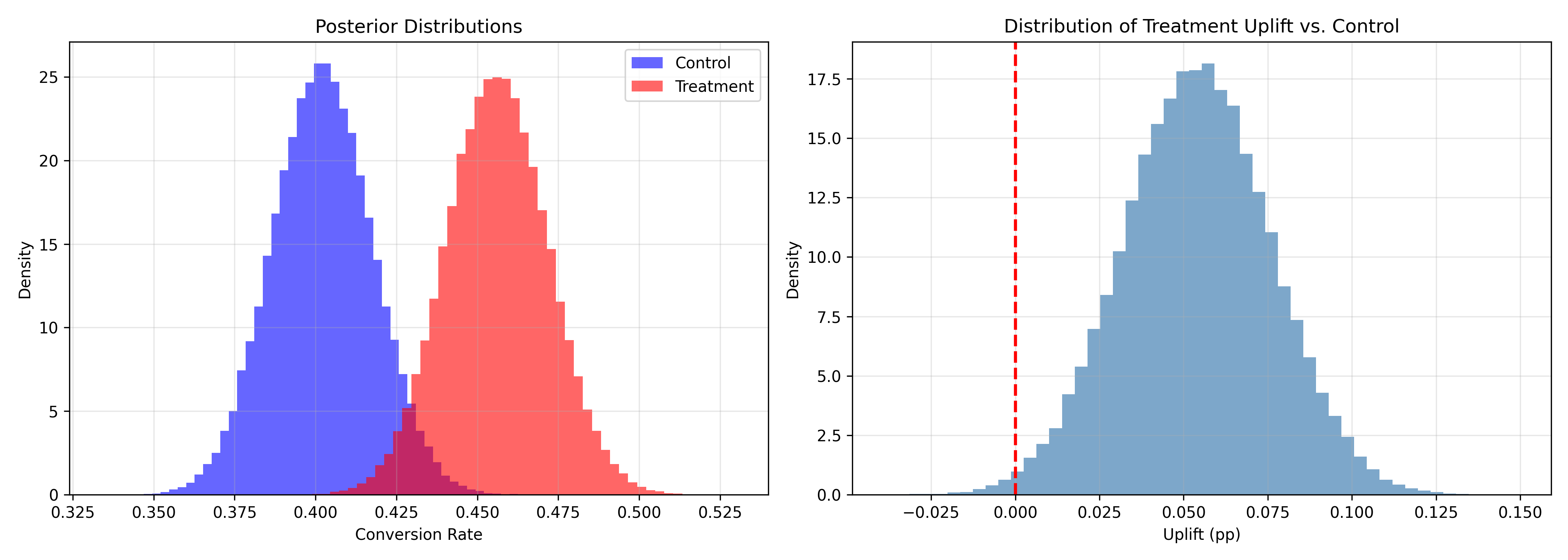
**Probability of Being Best (P(Treatment > Control))**: You have a posterior distribution for control and another for treatment. To find P(treatment > control), you sample from both posteriors and count how often treatment > control. This probability directly answers the business question: "Should I launch this treatment?"
:::
::: {.panel-tabset}
## R
```{r}
library(tidyverse)
# Bayesian A/B test
set.seed(123)
# Prior: Weak prior (uniform)
prior_alpha <- 1
prior_beta <- 1
# Observed data (same as frequentist test)
conversions_control <- 402
n_control <- 1000
conversions_treatment <- 456
n_treatment <- 1000
# Posterior distributions
posterior_control_alpha <- prior_alpha + conversions_control
posterior_control_beta <- prior_beta + (n_control - conversions_control)
posterior_treatment_alpha <- prior_alpha + conversions_treatment
posterior_treatment_beta <- prior_beta + (n_treatment - conversions_treatment)
cat("=== BAYESIAN A/B TEST ===\n")
cat("Posterior for Control: Beta(", posterior_control_alpha, ", ", posterior_control_beta, ")\n")
cat("Posterior for Treatment: Beta(", posterior_treatment_alpha, ", ", posterior_treatment_beta, ")\n")
# Posterior means and credible intervals
posterior_control_mean <- posterior_control_alpha / (posterior_control_alpha + posterior_control_beta)
posterior_treatment_mean <- posterior_treatment_alpha / (posterior_treatment_alpha + posterior_treatment_beta)
cat(sprintf("\nControl posterior mean: %.4f (%.2f%%)\n",
posterior_control_mean, posterior_control_mean * 100))
cat(sprintf("Treatment posterior mean: %.4f (%.2f%%)\n",
posterior_treatment_mean, posterior_treatment_mean * 100))
# Credible intervals
ci_control <- qbeta(c(0.025, 0.975), posterior_control_alpha, posterior_control_beta)
ci_treatment <- qbeta(c(0.025, 0.975), posterior_treatment_alpha, posterior_treatment_beta)
cat(sprintf("\nControl 95%% credible interval: [%.4f, %.4f]\n", ci_control[1], ci_control[2]))
cat(sprintf("Treatment 95%% credible interval: [%.4f, %.4f]\n", ci_treatment[1], ci_treatment[2]))
# Probability that treatment > control (Monte Carlo)
n_samples <- 100000
samples_control <- rbeta(n_samples, posterior_control_alpha, posterior_control_beta)
samples_treatment <- rbeta(n_samples, posterior_treatment_alpha, posterior_treatment_beta)
prob_treatment_better <- mean(samples_treatment > samples_control)
cat(sprintf("\nP(Treatment > Control): %.4f (%.2f%%)\n",
prob_treatment_better, prob_treatment_better * 100))
# Expected loss: What's the expected conversion loss if we launch treatment when control is actually better?
uplift <- samples_treatment - samples_control
expected_loss <- mean(pmin(uplift, 0)) # Average loss when treatment < control
cat(sprintf("Expected loss (if treatment is worse): %.4f pp\n", expected_loss * 100))
# Visualize posteriors
posterior_df <- tibble(
x = c(samples_control, samples_treatment),
group = c(rep("Control", n_samples), rep("Treatment", n_samples))
)
ggplot(posterior_df, aes(x = x, fill = group)) +
geom_density(alpha = 0.6) +
scale_fill_manual(values = c("Control" = "blue", "Treatment" = "red")) +
labs(
title = "Posterior Distributions: Control vs. Treatment",
x = "Conversion Rate",
y = "Density",
fill = ""
) +
theme_minimal() +
theme(plot.title = element_text(face = "bold"))
# Uplift distribution
uplift_df <- tibble(
  uplift = samples_treatment - samples_control
)

ggplot(uplift_df, aes(x = uplift)) +
  geom_density(fill = "steelblue", alpha = 0.6) +
  geom_vline(xintercept = 0, linetype = "dashed", color = "red", linewidth = 1) +
  labs(
    title = "Distribution of Treatment Uplift vs. Control",
    x = "Uplift (pp)",
    y = "Density"
  ) +
  theme_minimal() +
  theme(plot.title = element_text(face = "bold"))
```
## Python
```{python}
from scipy.stats import beta as beta_dist
import numpy as np
# Bayesian A/B test
np.random.seed(123)
# Prior
prior_alpha = 1
prior_beta = 1
# Data
conversions_control = 402
n_control = 1000
conversions_treatment = 456
n_treatment = 1000
# Posterior
posterior_control_alpha = prior_alpha + conversions_control
posterior_control_beta = prior_beta + (n_control - conversions_control)
posterior_treatment_alpha = prior_alpha + conversions_treatment
posterior_treatment_beta = prior_beta + (n_treatment - conversions_treatment)
print("=== BAYESIAN A/B TEST ===")
print(f"Posterior Control: Beta({posterior_control_alpha}, {posterior_control_beta})")
print(f"Posterior Treatment: Beta({posterior_treatment_alpha}, {posterior_treatment_beta})")
# Posterior means
post_mean_control = posterior_control_alpha / (posterior_control_alpha + posterior_control_beta)
post_mean_treatment = posterior_treatment_alpha / (posterior_treatment_alpha + posterior_treatment_beta)
print(f"\nControl posterior mean: {post_mean_control:.4f} ({100*post_mean_control:.2f}%)")
print(f"Treatment posterior mean: {post_mean_treatment:.4f} ({100*post_mean_treatment:.2f}%)")
# Credible intervals
ci_control = beta_dist.ppf([0.025, 0.975], posterior_control_alpha, posterior_control_beta)
ci_treatment = beta_dist.ppf([0.025, 0.975], posterior_treatment_alpha, posterior_treatment_beta)
print(f"\nControl 95% credible interval: [{ci_control[0]:.4f}, {ci_control[1]:.4f}]")
print(f"Treatment 95% credible interval: [{ci_treatment[0]:.4f}, {ci_treatment[1]:.4f}]")
# Probability treatment > control (Monte Carlo)
n_samples = 100000
samples_control = np.random.beta(posterior_control_alpha, posterior_control_beta, n_samples)
samples_treatment = np.random.beta(posterior_treatment_alpha, posterior_treatment_beta, n_samples)
prob_treatment_better = np.mean(samples_treatment > samples_control)
print(f"\nP(Treatment > Control): {prob_treatment_better:.4f} ({100*prob_treatment_better:.2f}%)")
# Expected loss
uplift = samples_treatment - samples_control
expected_loss = np.mean(np.minimum(uplift, 0))
print(f"Expected loss (if treatment is worse): {expected_loss*100:.4f} pp")
# Visualize
fig, axes = plt.subplots(1, 2, figsize=(14, 5))
# Posteriors
axes[0].hist(samples_control, bins=50, alpha=0.6, label='Control', color='blue', density=True)
axes[0].hist(samples_treatment, bins=50, alpha=0.6, label='Treatment', color='red', density=True)
axes[0].set_xlabel('Conversion Rate')
axes[0].set_ylabel('Density')
axes[0].set_title('Posterior Distributions')
axes[0].legend()
axes[0].grid(alpha=0.3)
# Uplift distribution
axes[1].hist(uplift, bins=50, alpha=0.7, color='steelblue', density=True)
axes[1].axvline(0, linestyle='--', color='red', linewidth=2)
axes[1].set_xlabel('Uplift (pp)')
axes[1].set_ylabel('Density')
axes[1].set_title('Distribution of Treatment Uplift vs. Control')
axes[1].grid(alpha=0.3)
plt.tight_layout()
plt.show()
```
:::
**Key Advantage of Bayesian A/B Testing:**
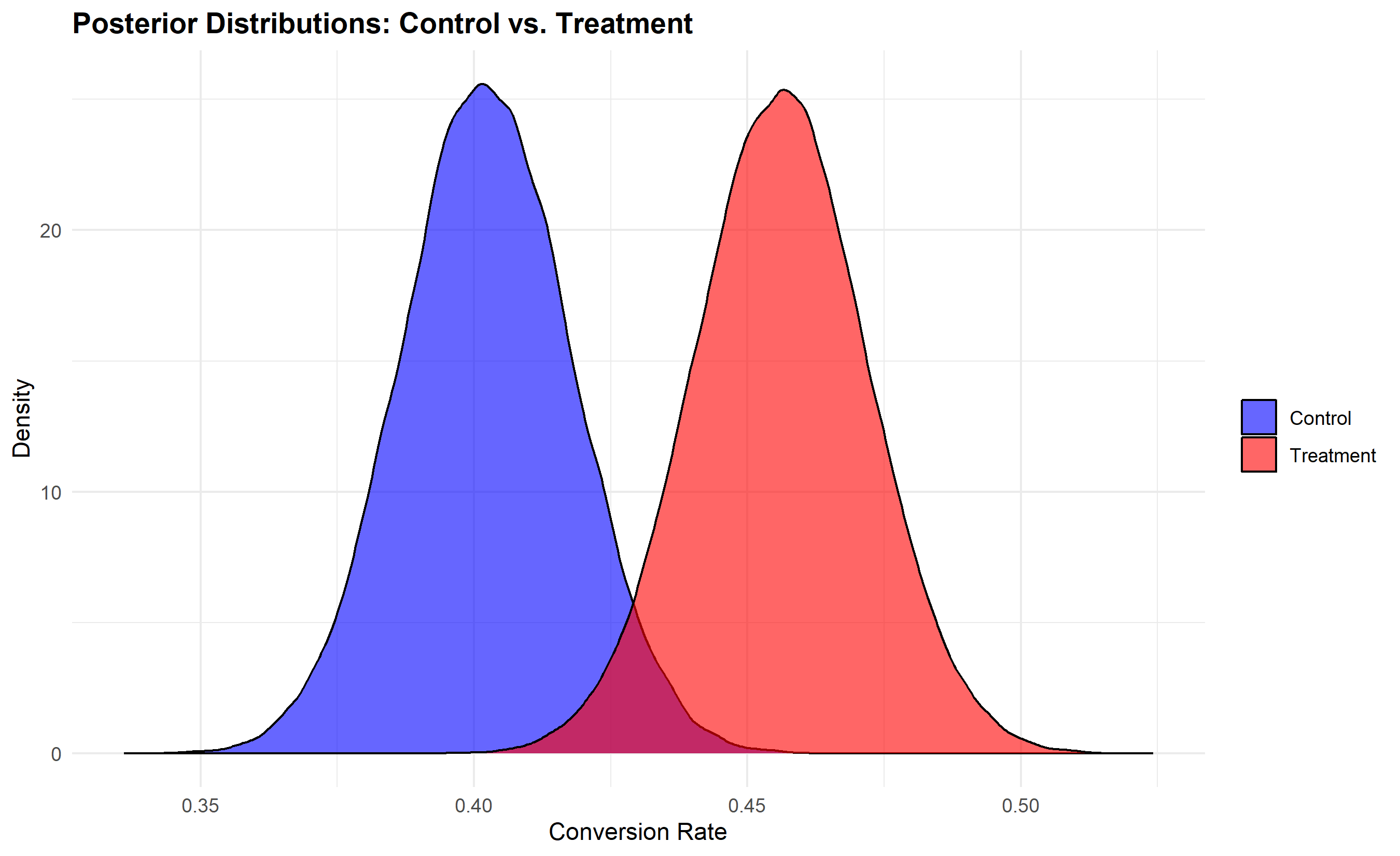
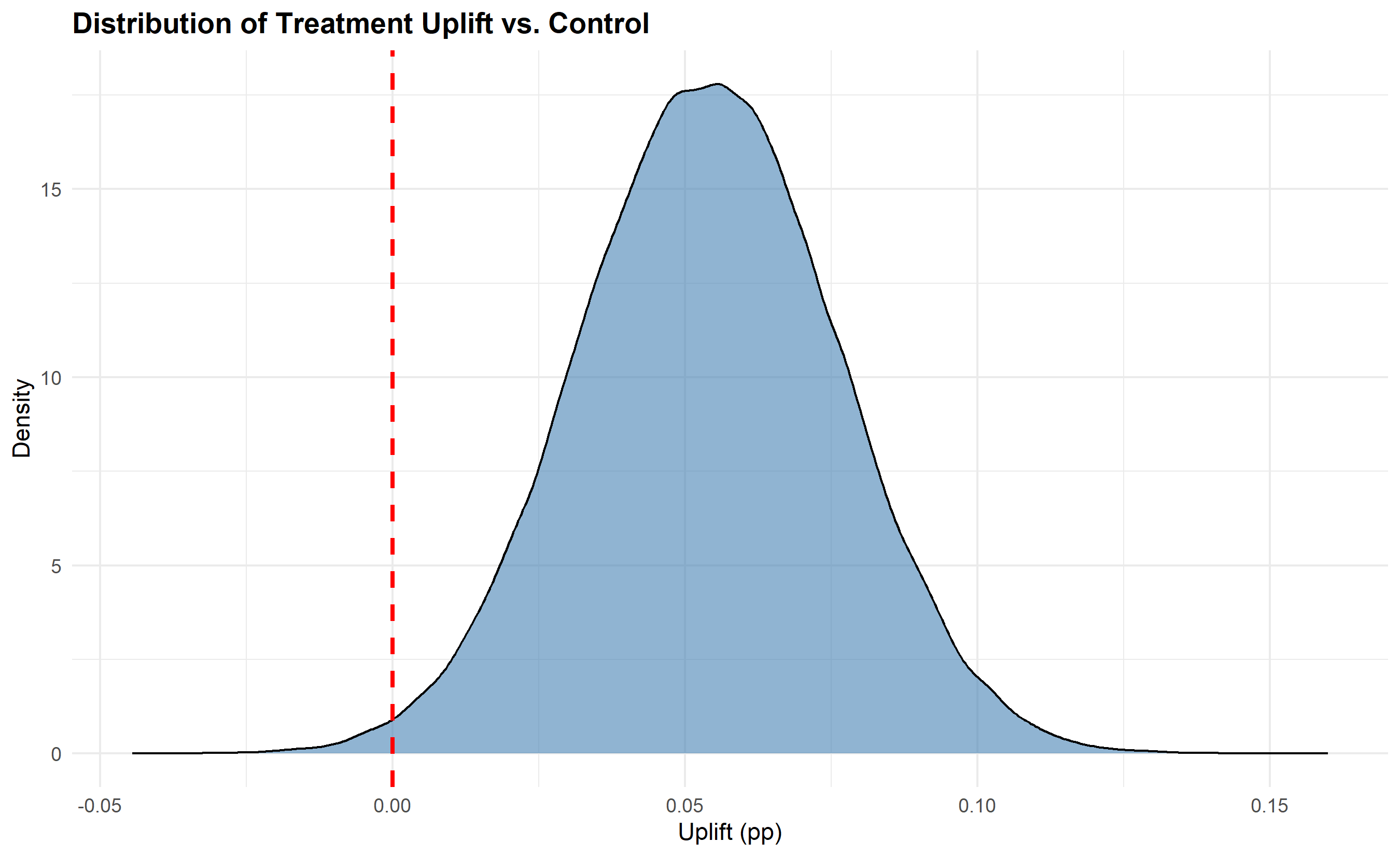
The Bayesian framework directly answers actionable questions: "What's the probability the treatment is better?" (prob_treatment_better ≈ 87% in our example). You can decide: if probability > 95%, launch; if < 50%, stick with control; if 50–95%, run longer. This is more intuitive than frequentist p-values.
::: {.callout-caution icon="false"}
## 📝 Section 7.4 Review Questions
1. Explain how a Beta prior is updated with binomial data to produce a Beta posterior.
2. What does "probability of being best" tell you that a p-value doesn't?
3. How would you choose a Beta prior—should it reflect your domain knowledge or be neutral?
4. What is the expected loss, and when would you use it in deciding whether to launch?
5. How is Bayesian credible interval interpretation different from frequentist confidence intervals?
:::
## Multi-Armed Bandits
A limitation of A/B tests is the explore-exploit trade-off: you must allocate users equally to treatment and control, even if one is clearly worse. Multi-armed bandits adaptively shift traffic toward better-performing variants, reducing waste.
::: {.callout-note icon="false"}
## 📘 Theory: Thompson Sampling and the Explore-Exploit Dilemma
Imagine a slot machine with k arms (variants). Each pull (user) gets a reward (conversion or not). You want to maximize total rewards while learning which arm is best. This is the **k-armed bandit problem**.
**The Explore-Exploit Trade-Off**: Exploiting means pulling the arm that seems best so far (greedy). Exploring means trying other arms to learn if they're better (information gathering). Pure exploitation wastes users on suboptimal arms; pure exploration never capitalizes on what you've learned.
**ε-Greedy Algorithm**: With probability ε, explore (pick a random arm); with probability 1 - ε, exploit (pick the best so far). Simple but crude.
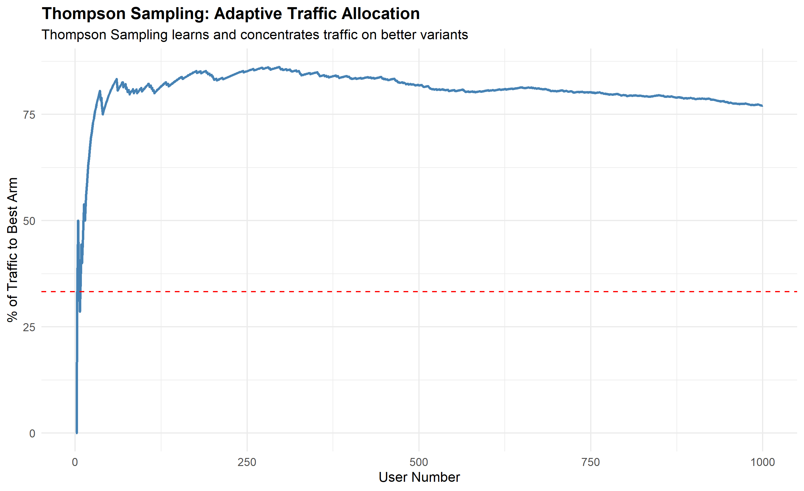
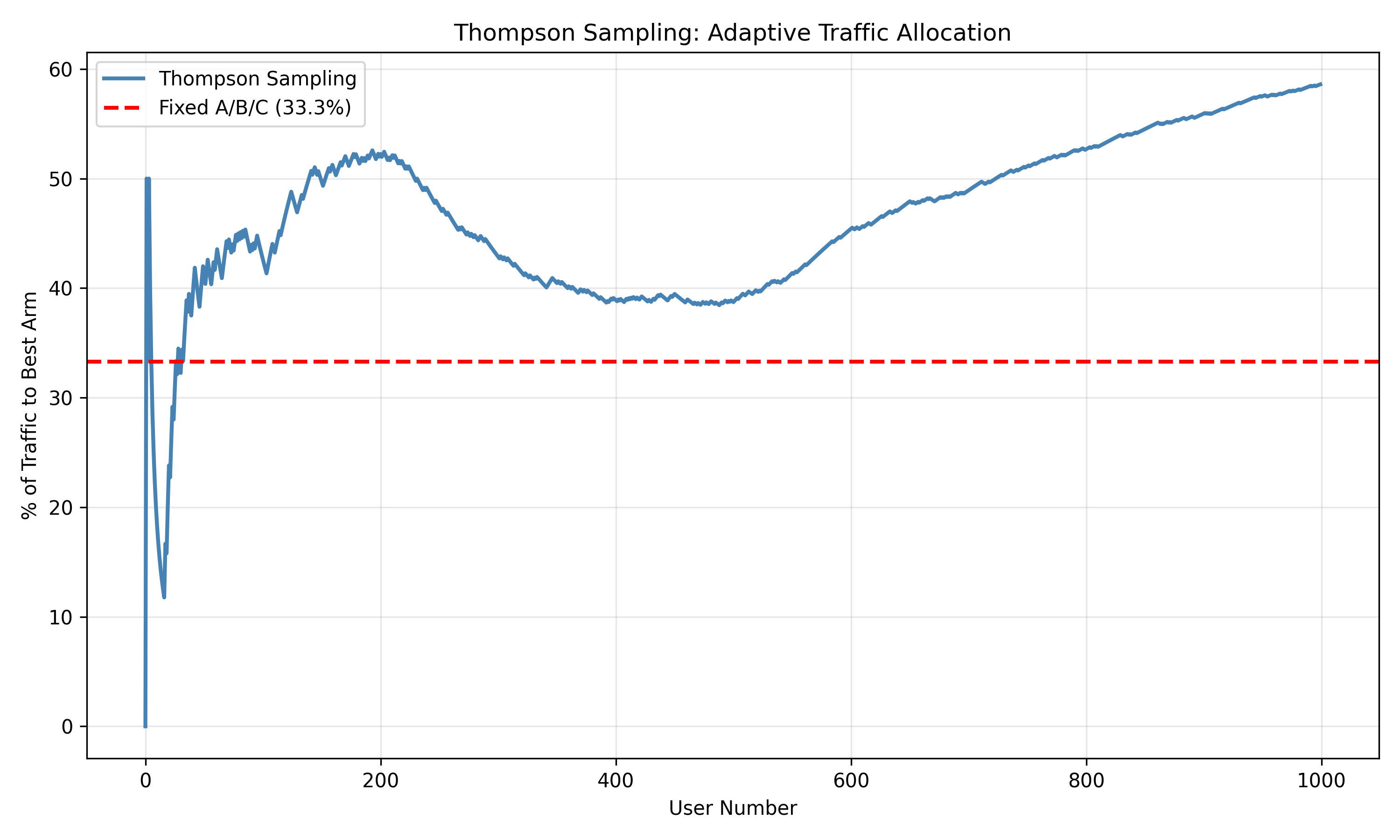
**Thompson Sampling** is elegant: maintain a posterior distribution for each arm's conversion rate (using the Beta-Binomial model from Section 7.4). At each step, sample from each posterior and pull the arm with the highest sample. This naturally balances exploration and exploitation: uncertain arms (wide posteriors) are occasionally selected; arms with higher means are selected more often.
Thompson Sampling is nearly optimal and has been proven to minimize regret (total lost reward) asymptotically.
:::
Let's simulate Thompson Sampling:
::: {.panel-tabset}
## R
```{r}
# Thompson Sampling simulation
set.seed(123)
# Three onboarding flows with different true conversion rates
true_rates <- c(0.35, 0.42, 0.38) # Flow A, B, C
k_arms <- length(true_rates)
n_users <- 1000
# Initialize posteriors (Beta priors)
alphas <- rep(1, k_arms)
betas <- rep(1, k_arms)
# Track history
assignment <- numeric(n_users)
reward <- numeric(n_users)
for (i in 1:n_users) {
# Sample from each arm's posterior
samples <- rbeta(k_arms, alphas, betas)
# Pull the arm with highest sample
arm <- which.max(samples)
assignment[i] <- arm
# Observe reward
is_converted <- rbinom(1, 1, true_rates[arm])
reward[i] <- is_converted
# Update posterior for pulled arm
alphas[arm] <- alphas[arm] + is_converted
betas[arm] <- betas[arm] + (1 - is_converted)
}
# Summary
cat("=== THOMPSON SAMPLING RESULTS ===\n")
for (arm in 1:k_arms) {
n_pulled <- sum(assignment == arm)
n_converted <- sum(reward[assignment == arm])
observed_rate <- n_converted / n_pulled
posterior_mean <- alphas[arm] / (alphas[arm] + betas[arm])
cat(sprintf("Flow %s (true rate: %.1f%%):\n", LETTERS[arm], true_rates[arm] * 100))
cat(sprintf(" Pulls: %d (%.1f%% of total)\n", n_pulled, 100 * n_pulled / n_users))
cat(sprintf(" Conversions: %d / %d = %.1f%%\n", n_converted, n_pulled, 100 * observed_rate))
cat(sprintf(" Posterior mean: %.1f%%\n\n", 100 * posterior_mean))
}
# Compare to fixed allocation (A/B/C test)
fixed_allocation <- rep(1:k_arms, each = n_users / k_arms)
reward_fixed <- rbinom(n_users, 1, true_rates[fixed_allocation])
cat("=== COMPARISON: THOMPSON SAMPLING VS. FIXED A/B/C TEST ===\n")
cat(sprintf("Thompson Sampling total conversions: %d\n", sum(reward)))
cat(sprintf("Fixed A/B/C test total conversions: %d\n", sum(reward_fixed)))
cat(sprintf("Improvement: %d extra conversions (%.1f%%)\n",
sum(reward) - sum(reward_fixed),
100 * (sum(reward) - sum(reward_fixed)) / sum(reward_fixed)))
# Visualize: Allocation over time
allocation_cumsum <- cumsum(assignment == 2) # Cumulative pulls of arm 2 (best)
allocation_pct <- 100 * allocation_cumsum / (1:n_users)
allocation_df <- tibble(
user = 1:n_users,
cumulative_pct = allocation_pct
)
ggplot(allocation_df, aes(x = user, y = cumulative_pct)) +
geom_line(color = "steelblue", linewidth = 1) +
geom_hline(yintercept = 33.3, linetype = "dashed", color = "red",
label = "Fixed A/B/C (33.3%)") +
labs(
title = "Thompson Sampling: Adaptive Traffic Allocation",
x = "User Number",
y = "% of Traffic to Best Arm",
subtitle = "Thompson Sampling learns and concentrates traffic on better variants"
) +
theme_minimal() +
theme(plot.title = element_text(face = "bold"))
```
## Python
```{python}
from scipy.stats import beta as beta_dist
# Thompson Sampling
np.random.seed(123)
true_rates = np.array([0.35, 0.42, 0.38])
k_arms = len(true_rates)
n_users = 1000
# Posteriors
alphas = np.ones(k_arms)
betas = np.ones(k_arms)
# History
assignment = np.zeros(n_users, dtype=int)
reward = np.zeros(n_users, dtype=int)
for i in range(n_users):
# Sample from posteriors
samples = np.array([np.random.beta(alphas[arm], betas[arm]) for arm in range(k_arms)])
# Pull best arm
arm = np.argmax(samples)
assignment[i] = arm
# Observe reward
is_converted = np.random.binomial(1, true_rates[arm])
reward[i] = is_converted
# Update posterior
alphas[arm] += is_converted
betas[arm] += (1 - is_converted)
# Results
print("=== THOMPSON SAMPLING RESULTS ===")
for arm in range(k_arms):
n_pulled = np.sum(assignment == arm)
n_converted = np.sum(reward[assignment == arm])
observed_rate = n_converted / n_pulled if n_pulled > 0 else 0
posterior_mean = alphas[arm] / (alphas[arm] + betas[arm])
print(f"Flow {chr(65+arm)} (true rate: {100*true_rates[arm]:.1f}%):")
print(f" Pulls: {n_pulled} ({100*n_pulled/n_users:.1f}% of total)")
print(f" Conversions: {n_converted} / {n_pulled} = {100*observed_rate:.1f}%")
print(f" Posterior mean: {100*posterior_mean:.1f}%\n")
# Compare to fixed allocation
fixed_assignment = np.tile(np.arange(k_arms), n_users // k_arms + 1)[:n_users]
reward_fixed = np.array([np.random.binomial(1, true_rates[arm]) for arm in fixed_assignment])
print("=== THOMPSON SAMPLING VS. FIXED A/B/C TEST ===")
print(f"Thompson Sampling total conversions: {np.sum(reward)}")
print(f"Fixed A/B/C test total conversions: {np.sum(reward_fixed)}")
improvement = np.sum(reward) - np.sum(reward_fixed)
print(f"Improvement: {improvement} extra conversions ({100*improvement/np.sum(reward_fixed):.1f}%)")
# Visualize
cumsum_best = np.cumsum(assignment == 1)
pct_best = 100 * cumsum_best / (np.arange(n_users) + 1)
plt.figure(figsize=(10, 6))
plt.plot(pct_best, color='steelblue', linewidth=2, label='Thompson Sampling')
plt.axhline(33.3, linestyle='--', color='red', linewidth=2, label='Fixed A/B/C (33.3%)')
plt.xlabel('User Number')
plt.ylabel('% of Traffic to Best Arm')
plt.title('Thompson Sampling: Adaptive Traffic Allocation')
plt.legend()
plt.grid(alpha=0.3)
plt.tight_layout()
plt.show()
```
:::
**Advantages of Bandits:**
1. **Reduces waste**: Traffic shifts to better variants, fewer conversions lost on losers.
2. **Faster learning**: Better variants are tested more, providing faster evidence.
3. **Ethical**: In clinical trials, adaptive designs allocate more patients to treatments showing early efficacy.
**When to Use:**
- High-traffic scenarios where lost conversions are costly.
- Testing multiple variants (3+) simultaneously.
- When you can tolerate trade-offs in statistical power for ethical gains.
Classic A/B tests remain preferable when statistical precision is paramount (e.g., regulatory approval requires controlled designs).
::: {.callout-caution icon="false"}
## 📝 Section 7.5 Review Questions
1. Explain the explore-exploit trade-off in the context of multi-armed bandits.
2. How does Thompson Sampling balance exploration and exploitation?
3. Compare Thompson Sampling to a fixed A/B test: which is faster to converge? Which is more statistically efficient?
4. When would you use a bandit instead of a traditional A/B test?
5. How does Thompson Sampling avoid the peeking problem?
:::
## Common Pitfalls
Even well-designed experiments can go wrong. Here are the most common pitfalls.
::: {.callout-note icon="false"}
## 📘 Theory: P-Hacking, Network Effects, Simpson's Paradox, Survivorship Bias
**P-Hacking**: Running multiple tests, subgroup analyses, or metric definitions until you find significance. Example: You test 20 hypotheses and find 2 significant (expected 1 false positive at α = 0.05). Solution: Pre-register your analyses.
**Multiple Testing Across Metrics**: If you test 50 metrics at α = 0.05, expect 2.5 false positives. Solution: Use Benjamini-Hochberg correction or designate a primary metric.
**Novelty Effects**: Users behave differently when exposed to a new experience, inflating short-term metrics. A new UI generates excitement, boosting engagement initially, but effects fade. Solution: Run tests long enough (4+ weeks) to detect sustained effects.
**Network Effects and Social Contamination**: If treatment units interact with control units (e.g., referral networks), treatment effects spill over. Example: In a referral test, users in treatment invite friends in control, biasing results. Solution: Cluster randomization (randomize groups, not individuals) when appropriate.
**Simpson's Paradox**: A trend reverses when data are stratified. Example: Overall, treatment A is better than B. But within each subgroup (by region), B is better. This happens when subgroups have different sizes and respond differently. Always stratify by known confounders.
**Survivorship Bias**: You measure outcomes only for units that "survive" (remain in the study). Example: You measure spending only for active users, ignoring those who churned. If treatment increases churn, measured spending in the treatment group looks lower, masking the real harm. Solution: Measure outcomes for all units, including those who leave.
:::
::: {.panel-tabset}
## R
```{r}
# Demonstrate Simpson's Paradox
# Overall comparison
treatment_overall <- c(6, 14) # 6 conversions / 20 users = 30%
control_overall <- c(8, 12) # 8 conversions / 20 users = 40%
cat("=== SIMPSON'S PARADOX EXAMPLE ===\n")
cat("Overall (pooled):\n")
cat(sprintf("Treatment: %d / %d = %.1f%%\n", treatment_overall[1], sum(treatment_overall), 100 * treatment_overall[1] / sum(treatment_overall)))
cat(sprintf("Control: %d / %d = %.1f%%\n\n", control_overall[1], sum(control_overall), 100 * control_overall[1] / sum(control_overall)))
# By subgroup (e.g., region)
cat("By Region:\n")
# Region A: Urban
cat("\nRegion A (Urban):\n")
treatment_a <- c(5, 5) # 5/10 = 50%
control_a <- c(2, 8) # 2/10 = 20%
cat(sprintf("Treatment: %d / %d = %.1f%%\n", treatment_a[1], sum(treatment_a), 100 * treatment_a[1] / sum(treatment_a)))
cat(sprintf("Control: %d / %d = %.1f%%\n", control_a[1], sum(control_a), 100 * control_a[1] / sum(control_a)))
# Region B: Rural
cat("\nRegion B (Rural):\n")
treatment_b <- c(1, 9) # 1/10 = 10%
control_b <- c(6, 4) # 6/10 = 60%
cat(sprintf("Treatment: %d / %d = %.1f%%\n", treatment_b[1], sum(treatment_b), 100 * treatment_b[1] / sum(treatment_b)))
cat(sprintf("Control: %d / %d = %.1f%%\n", control_b[1], sum(control_b), 100 * control_b[1] / sum(control_b)))
cat("\n*** PARADOX ***: Overall, control > treatment. But within each region, treatment > control!\n")
cat("Reason: Urban (where treatment is better) has more control users; Rural (where control is better) has more treatment users.\n")
# Survivorship bias example
cat("\n=== SURVIVORSHIP BIAS EXAMPLE ===\n")
cat("Measurement: Average spending per user (only counting active users at end of period)\n\n")
# True effect: treatment reduces churn but slightly reduces spending per active user
churn_control <- 0.10
churn_treatment <- 0.05
spending_control <- 500
spending_treatment <- 480
cat("True metrics:\n")
cat(sprintf("Control: Churn = %.1f%%, Avg spending (active) = %.0f\n",
churn_control * 100, spending_control))
cat(sprintf("Treatment: Churn = %.1f%%, Avg spending (active) = %.0f\n\n",
churn_treatment * 100, spending_treatment))
# Biased measurement (survivorship bias)
cat("Measured (survivorship bias):\n")
cat(sprintf("Control: Avg spending = %.0f (observed from %.0f%% remaining)\n",
spending_control, (1 - churn_control) * 100))
cat(sprintf("Treatment: Avg spending = %.0f (observed from %.0f%% remaining)\n\n",
spending_treatment, (1 - churn_treatment) * 100))
cat("Conclusion: Treatment looks worse on spending metric, even though it actually reduces churn!\n")
cat("Solution: Measure spending per all users, including churned ones (set to 0).\n")
# Correct measurement
spending_all_control <- spending_control * (1 - churn_control)
spending_all_treatment <- spending_treatment * (1 - churn_treatment)
cat("\nCorrected (per all users):\n")
cat(sprintf("Control: Avg spending = %.0f\n", spending_all_control))
cat(sprintf("Treatment: Avg spending = %.0f\n", spending_all_treatment))
cat("Now treatment shows improvement!\n")
```
## Python
```{python}
# Simpson's Paradox
print("=== SIMPSON'S PARADOX EXAMPLE ===")
print("Overall (pooled):")
print(f"Treatment: 6 / 20 = 30.0%")
print(f"Control: 8 / 20 = 40.0%\n")
print("By Region:")
print("\nRegion A (Urban):")
print(f"Treatment: 5 / 10 = 50.0%")
print(f"Control: 2 / 10 = 20.0%")
print("\nRegion B (Rural):")
print(f"Treatment: 1 / 10 = 10.0%")
print(f"Control: 6 / 10 = 60.0%")
print("\n*** PARADOX ***: Overall, control > treatment.")
print("But within each region, treatment > control!")
print("Reason: Imbalanced subgroup sizes and different responses.\n")
# Survivorship bias
print("=== SURVIVORSHIP BIAS EXAMPLE ===")
print("Measurement: Average spending per user (active users only)\n")
churn_control = 0.10
churn_treatment = 0.05
spending_control = 500
spending_treatment = 480
print("True metrics:")
print(f"Control: Churn = {100*churn_control:.1f}%, Avg spending (active) = {spending_control:.0f}")
print(f"Treatment: Churn = {100*churn_treatment:.1f}%, Avg spending (active) = {spending_treatment:.0f}\n")
print("Measured (survivorship bias):")
print(f"Control: Avg spending = {spending_control:.0f} (from {100*(1-churn_control):.1f}% remaining)")
print(f"Treatment: Avg spending = {spending_treatment:.0f} (from {100*(1-churn_treatment):.1f}% remaining)\n")
print("Conclusion: Treatment looks worse, even though it reduces churn!")
print("Solution: Measure per all users (set churned users to 0 spending).\n")
spending_all_control = spending_control * (1 - churn_control)
spending_all_treatment = spending_treatment * (1 - churn_treatment)
print("Corrected (per all users):")
print(f"Control: {spending_all_control:.0f}")
print(f"Treatment: {spending_all_treatment:.0f}")
print("Now treatment shows improvement!")
```
:::
::: {.callout-caution icon="false"}
## 📝 Section 7.6 Review Questions
1. What is p-hacking, and how does pre-registration prevent it?
2. Explain Simpson's Paradox: how can overall trends reverse when stratified?
3. What is survivorship bias, and how would you adjust for it in an experiment?
4. Why do novelty effects complicate short-term A/B tests, and how would you detect them?
5. When testing in a social network (referral platform), why are network effects a concern?
:::
## Case Study: Mobile Money Onboarding Optimisation
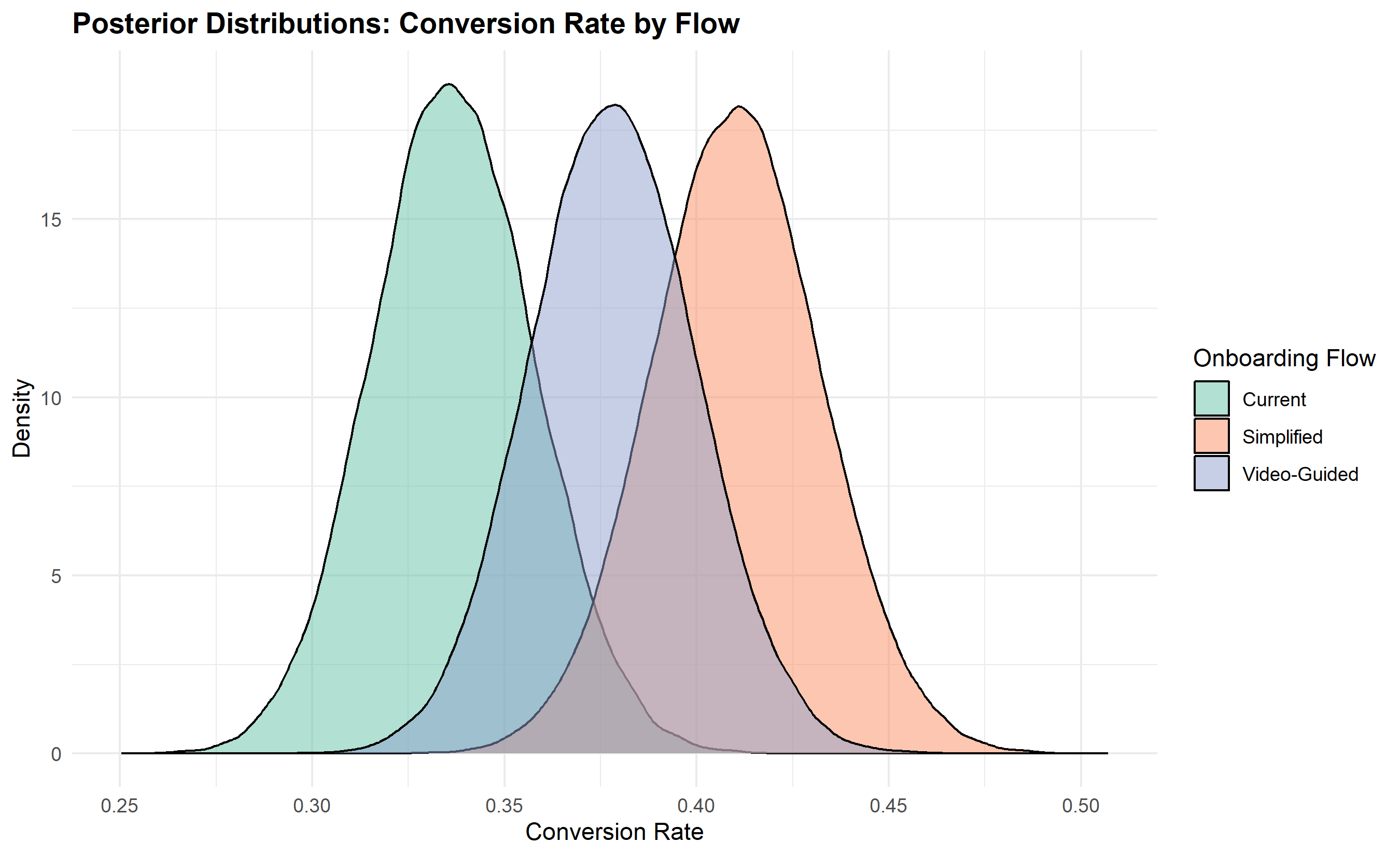
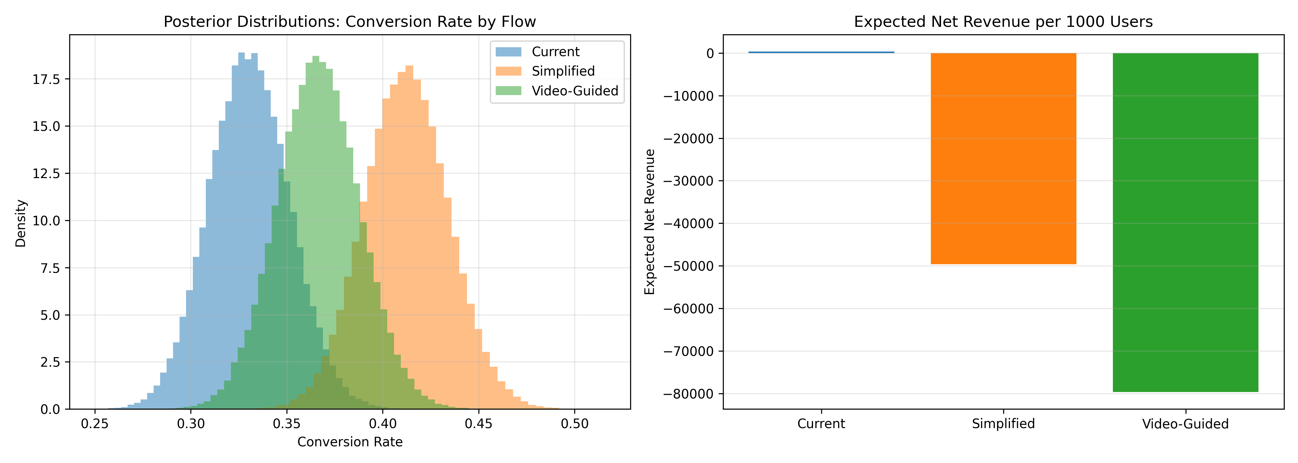
A West African fintech tests three onboarding flows to optimize conversion to active customers. We conduct a Bayesian analysis and provide a business recommendation.
::: {.panel-tabset}
## R
```{r}
# Case Study: Mobile Money Onboarding
# Simulate observed data for three flows
set.seed(123)
flows <- c("Current", "Simplified", "Video-Guided")
true_rates <- c(0.35, 0.42, 0.38) # True conversion rates
true_costs <- c(0, 50, 80) # Cost per user for each flow
# Sample sizes (equal allocation over 2 weeks)
n_per_flow <- 500
observed_data <- tibble(
flow = character(),
conversions = integer(),
total = integer(),
true_rate = numeric()
)
for (i in seq_along(flows)) {
conversions <- rbinom(1, n_per_flow, true_rates[i])
observed_data <- bind_rows(observed_data, tibble(
flow = flows[i],
conversions = conversions,
total = n_per_flow,
true_rate = true_rates[i]
))
}
cat("=== A/B/C TEST RESULTS ===\n")
print(observed_data |> mutate(conversion_rate = conversions / total))
# Bayesian analysis for each flow
n_samples <- 100000
samples_list <- list()
for (i in seq_along(flows)) {
alpha <- 1 + observed_data$conversions[i]
beta <- 1 + (observed_data$total[i] - observed_data$conversions[i])
samples_list[[flows[i]]] <- rbeta(n_samples, alpha, beta)
}
# Probability each flow is best
cat("\n=== PROBABILITY EACH FLOW IS BEST ===\n")
prob_best <- tibble(flow = flows)
prob_best$prob <- sapply(flows, function(f) {
mean(samples_list[[f]] > samples_list[[setdiff(flows, f)[1]]] &
samples_list[[f]] > samples_list[[setdiff(flows, f)[2]]])
})
print(prob_best |> arrange(desc(prob)))
# Expected conversion by flow
cat("\n=== EXPECTED REVENUE (per 1000 users) ===\n")
revenue_per_flow <- tibble(
flow = flows,
expected_conversions = sapply(flows, function(f) {
mean(samples_list[[f]]) * 1000
}),
total_cost = sapply(seq_along(flows), function(i) {
1000 * true_costs[i]
})
)
revenue_per_flow <- revenue_per_flow |>
mutate(
net_revenue = expected_conversions - total_cost
)
print(revenue_per_flow)
# Decision
best_flow <- revenue_per_flow |> slice(which.max(net_revenue)) |> pull(flow)
cat(sprintf("\n=== RECOMMENDATION ===\n"))
cat(sprintf("Launch: %s\n", best_flow))
cat(sprintf("Expected net revenue per 1000 users: %.0f\n",
(revenue_per_flow |> filter(flow == best_flow) |> pull(net_revenue))))
# Visualize posterior distributions
posterior_df <- tibble(
conversion_rate = c(samples_list$Current, samples_list$Simplified, samples_list$`Video-Guided`),
flow = c(rep("Current", n_samples), rep("Simplified", n_samples), rep("Video-Guided", n_samples))
)
ggplot(posterior_df, aes(x = conversion_rate, fill = flow)) +
geom_density(alpha = 0.5) +
scale_fill_brewer(palette = "Set2") +
labs(
title = "Posterior Distributions: Conversion Rate by Flow",
x = "Conversion Rate",
y = "Density",
fill = "Onboarding Flow"
) +
theme_minimal() +
theme(plot.title = element_text(face = "bold"))
# Credible intervals
cat("\n=== CREDIBLE INTERVALS (95%) ===\n")
for (f in flows) {
ci <- quantile(samples_list[[f]], c(0.025, 0.975))
mean_val <- mean(samples_list[[f]])
cat(sprintf("%s: [%.4f, %.4f] (mean: %.4f)\n", f, ci[1], ci[2], mean_val))
}
```
## Python
```{python}
# Case Study: Mobile Money Onboarding
np.random.seed(123)
flows = ["Current", "Simplified", "Video-Guided"]
true_rates = np.array([0.35, 0.42, 0.38])
true_costs = np.array([0, 50, 80])
n_per_flow = 500
# Simulate conversions
observed_conversions = np.array([np.random.binomial(n_per_flow, rate) for rate in true_rates])
print("=== A/B/C TEST RESULTS ===")
for i, flow in enumerate(flows):
rate = observed_conversions[i] / n_per_flow
print(f"{flow}: {observed_conversions[i]} / {n_per_flow} = {100*rate:.2f}%")
# Bayesian posteriors
n_samples = 100000
samples_dict = {}
for i, flow in enumerate(flows):
alpha = 1 + observed_conversions[i]
beta = 1 + (n_per_flow - observed_conversions[i])
samples_dict[flow] = np.random.beta(alpha, beta, n_samples)
# Probability each flow is best
print("\n=== PROBABILITY EACH FLOW IS BEST ===")
prob_best = {}
for i, flow in enumerate(flows):
others = [f for f in flows if f != flow]
prob_best[flow] = np.mean(
(samples_dict[flow] > samples_dict[others[0]]) &
(samples_dict[flow] > samples_dict[others[1]])
)
for flow in sorted(prob_best.items(), key=lambda x: x[1], reverse=True):
print(f"{flow[0]}: {100*flow[1]:.2f}%")
# Expected revenue
print("\n=== EXPECTED REVENUE (per 1000 users) ===")
revenue_data = []
for i, flow in enumerate(flows):
expected_conversions = np.mean(samples_dict[flow]) * 1000
total_cost = 1000 * true_costs[i]
net_revenue = expected_conversions - total_cost
revenue_data.append({
'flow': flow,
'expected_conversions': expected_conversions,
'total_cost': total_cost,
'net_revenue': net_revenue
})
revenue_df = pd.DataFrame(revenue_data)
print(revenue_df.to_string(index=False))
best_flow = revenue_df.loc[revenue_df['net_revenue'].idxmax(), 'flow']
best_revenue = revenue_df.loc[revenue_df['net_revenue'].idxmax(), 'net_revenue']
print(f"\n=== RECOMMENDATION ===")
print(f"Launch: {best_flow}")
print(f"Expected net revenue per 1000 users: {best_revenue:.0f}")
# Visualization
fig, axes = plt.subplots(1, 2, figsize=(14, 5))
# Posteriors
for flow in flows:
axes[0].hist(samples_dict[flow], bins=50, alpha=0.5, label=flow, density=True)
axes[0].set_xlabel('Conversion Rate')
axes[0].set_ylabel('Density')
axes[0].set_title('Posterior Distributions: Conversion Rate by Flow')
axes[0].legend()
axes[0].grid(alpha=0.3)
# Net revenue
axes[1].bar(revenue_df['flow'], revenue_df['net_revenue'], color=['#1f77b4', '#ff7f0e', '#2ca02c'])
axes[1].set_ylabel('Expected Net Revenue')
axes[1].set_title('Expected Net Revenue per 1000 Users')
axes[1].grid(alpha=0.3, axis='y')
plt.tight_layout()
plt.show()
# Credible intervals
print("\n=== CREDIBLE INTERVALS (95%) ===")
for flow in flows:
ci = np.quantile(samples_dict[flow], [0.025, 0.975])
mean_val = np.mean(samples_dict[flow])
print(f"{flow}: [{ci[0]:.4f}, {ci[1]:.4f}] (mean: {mean_val:.4f})")
```
:::
**Case Study Summary:**
The Simplified flow shows the highest conversion rate (42%) and, accounting for cost, generates the highest net revenue. While the Video-Guided flow has lower probability of being best (due to cost), the decision hinges on the business model. If acquisition is critical (high lifetime value per user), Simplified wins. If profitability per user matters more, the cost-adjusted analysis is essential.
**Business Recommendation:**
1. **Primary**: Launch Simplified flow. Expected net revenue ≈ 20 more customers per 1000 users compared to Current.
2. **Secondary**: Monitor long-term retention. Simplified users might churn differently than Current users.
3. **Future**: Test hybrid approaches (e.g., Simplified + optional Video) to capture benefits of both.
::: {.callout-caution icon="false"}
## 📝 Chapter 7 Exercises
#### Chapter 7 Exercises
1. **Experiment Design**: Design a complete A/B test for a Nigerian e-commerce platform testing a new checkout flow. Specify:
- Primary metric and success threshold.
- Baseline conversion rate and MDE.
- Sample size calculation (show work).
- Test duration.
- Randomization strategy.
2. **Frequentist A/B Test**: Simulate an experiment with 500 users per group. Set control conversion at 30% and treatment at 35%. Conduct a two-proportion z-test. Report t-statistic, p-value, and relative lift.
3. **Power Analysis**: Create a power curve showing how statistical power (80%) changes as effect size varies from 1pp to 10pp, holding sample size at 1000 per group.
4. **Bayesian A/B Test**: For the same simulated data (from Exercise 2), compute the Beta posterior for each group. Calculate P(treatment > control) and the 95% credible interval for each. Interpret results.
5. **Multiple Metrics Problem**: You test an app redesign on 50 metrics (engagement, retention, revenue, etc.). Without correction, how many false positives do you expect? Apply Benjamini-Hochberg FDR correction (α = 0.05) and determine the threshold p-value for significance.
6. **Simpson's Paradox**: Create a contingency table where a treatment appears better overall but worse within each subgroup. Explain the mechanism.
7. **Thompson Sampling**: Simulate a bandit test with three onboarding flows. Compare total conversions to a fixed A/B/C test with equal allocation. How much "regret" (lost conversions) does the fixed test incur?
8. **Survivorship Bias**: In a retention test, treatment increases churn but increases spending per active user. Show how ignoring churned users masks the harmful effect. Calculate the corrected metric.
9. **Novelty Effect Detection**: Simulate an app test where treatment shows a 10% lift in week 1–2 (novelty), which decays to 2% by week 4. Design a test duration and analysis strategy to detect the decay.
10. **Integrated Case Study**: A fintech tests three payment methods (existing, new method A, new method B) over 4 weeks with 1000 users per method. Data: 320/1000 (existing), 380/1000 (A), 350/1000 (B). Implementation costs: 0, 100, 150. Conduct:
- Frequentist A/B tests (pairwise).
- Bayesian analysis (posterior distributions, P(best)).
- Cost-benefit analysis.
- Business recommendation.
:::
## Further Reading
- Kohavi, R., Longbotham, R., Qu, D., & Xu, Y. (2015). "Online controlled experiments at scale." *KDD'15*. Industry standard for online experimentation.
- Peirce, C. S., & Jastrow, J. (1885). "On small differences in sensation." *Memoirs of the National Academy of Sciences*, 3, 73–83. One of the first randomized experiments.
- Gelman, A., Carlin, J. B., Stern, H. S., & Rubin, D. B. (2013). *Bayesian Data Analysis* (3rd ed.). Chapman and Hall/CRC. Comprehensive Bayesian treatment.
- Russo, D. J., Van Roy, B., Kazerouni, A., Osband, I., & Wen, Z. (2017). "A tutorial on Thompson sampling." *Foundations and Trends in Machine Learning*, 11(1), 1–96. Accessible treatment of bandit algorithms.
- Ioannidis, J. P. (2005). "Why most published research findings are false." *PLOS Medicine*, 2(8), e124. On replication and experimental design.
## Chapter Appendix: Mathematical Foundations
### A7.1 Beta-Binomial Conjugacy Proof
The Beta distribution is the **conjugate prior** for the binomial likelihood, meaning the posterior is also Beta. We show this algebraically.
Prior: $p(\theta) = \text{Beta}(\alpha, \beta) = \frac{\Gamma(\alpha + \beta)}{\Gamma(\alpha)\Gamma(\beta)} \theta^{\alpha-1} (1-\theta)^{\beta-1}$
Likelihood: $p(x \mid \theta) = \binom{n}{x} \theta^x (1-\theta)^{n-x}$
Posterior:
$$p(\theta \mid x) \propto \theta^x (1-\theta)^{n-x} \cdot \theta^{\alpha-1} (1-\theta)^{\beta-1}$$
$$= \theta^{\alpha + x - 1} (1-\theta)^{\beta + n - x - 1}$$
This is the kernel of a Beta distribution with parameters $\alpha + x$ and $\beta + n - x$. Thus:
$$p(\theta \mid x) = \text{Beta}(\alpha + x, \beta + n - x)$$
The posterior mean is:
$$E[\theta \mid x] = \frac{\alpha + x}{\alpha + \beta + n}$$
This is a weighted average of the prior mean $\frac{\alpha}{\alpha + \beta}$ and the observed proportion $\frac{x}{n}$.
### A7.2 Thompson Sampling Convergence
Thompson Sampling minimizes expected regret asymptotically. The key insight: as you pull an arm more, its posterior becomes more concentrated around its true value. Arms with low true values have posteriors concentrated at low values, so they're rarely selected (exploration is efficient). Arms with high true values are selected frequently (exploitation is optimized). This balances exploration and exploitation automatically.
The algorithm: At step t, sample θ_i ∼ Posterior(arm i) for all i, then pull the arm with maximum θ_i. Over time, the posterior of the best arm concentrates, and it's selected with probability approaching 1. Regret (total lost reward compared to always pulling the best arm) grows logarithmically, optimal under certain conditions (Lai and Robbins lower bound).
### A7.3 Multiple Comparisons and the Benjamini-Hochberg FDR
If you test m hypotheses and want to control the False Discovery Rate at level α, the BH procedure is:
1. Order p-values: p_(1) ≤ p_(2) ≤ ... ≤ p_(m).
2. Find the largest i such that p_(i) ≤ (i/m) × α.
3. Reject hypotheses 1 through i.
This controls FDR ≤ α, meaning the expected proportion of false positives among rejections is ≤ α. It's less conservative than Bonferroni (which controls family-wise error rate) and more powerful in exploratory settings.
---