---
title: "Topic Modelling, Text Classification, and Brand Analytics"
---
```{python}
#| label: python-setup-29-topic-modelling-brand
#| include: false
import numpy as np
import pandas as pd
import matplotlib.pyplot as plt
import seaborn as sns
from sklearn.feature_extraction.text import CountVectorizer, TfidfVectorizer
from sklearn.decomposition import LatentDirichletAllocation
from sklearn.linear_model import LogisticRegression
from sklearn.model_selection import train_test_split
from sklearn.metrics import confusion_matrix, classification_report, precision_recall_fscore_support
import random
import warnings
import re
# gensim is optional — used for coherence scoring; fall back gracefully if not installed
try:
from gensim.models import CoherenceModel, LdaModel, LdaMulticore
from gensim.corpora import Dictionary
import gensim.corpora as corpora
GENSIM_AVAILABLE = True
except ImportError:
GENSIM_AVAILABLE = False
print("Note: gensim not installed — coherence scoring will use sklearn LDA instead.")
from nltk.tokenize import word_tokenize
import nltk
```
::: {.callout-note icon="false"}
## 📋 Learning Objectives
By the end of this chapter, you will understand how to discover latent themes in unstructured text using topic models, classify documents into predefined categories with supervised learning, extract brand health signals from social media and customer communications, and apply speech recognition to operational call centre data. You will implement Latent Dirichlet Allocation (LDA) to automatically surface complaint categories from bank customer letters, train logistic regression classifiers on labelled customer service tickets, compute brand metrics from Twitter sentiment and topic distribution, and build an end-to-end workflow for complaint topic analysis linked to operational KPIs. The mathematical foundations include the Dirichlet distribution, collapsed Gibbs sampling, and perplexity as a model selection criterion. By project completion, you will have built reproducible pipelines for text mining at scale across both English and multilingual African datasets.
:::
## Topic Modelling as Unsupervised Text Mining
The volume of unstructured text generated by modern businesses far exceeds what human analysts can manually read and categorise. A mid-sized bank receives thousands of customer complaint letters, support tickets, and social media comments every week. A manufacturing firm tracks supplier communications, quality reports, and equipment failure narratives across dozens of plants. Traditional approaches—hiring teams to manually tag documents—do not scale. This is where topic modelling enters: an unsupervised machine learning technique that automatically discovers the underlying themes, or "topics," that run through a large text corpus without requiring pre-labelled examples.
Topic modelling rests on a deceptively simple intuition: documents are not random collections of words, but rather mixtures of a smaller number of recurring themes. A customer complaint about a malfunctioning ATM combines words like "machine," "cash," "not working," and "branch"—a latent topic we might label "ATM failures." Another letter about a delayed wire transfer uses "transfer," "money," "account," and "days"—a different topic. A single document often touches multiple topics: a complaint might mention both an ATM outage and a subsequent call centre wait time. By inferring these latent topics and their word probabilities, we can (1) automatically categorise documents, (2) discover unexpected themes in the data that were never explicitly labelled, (3) track how topic prevalence changes over time, and (4) segment customers or issues by their topic profiles for targeted business action.
The mathematical foundation is elegant: we model a topic as a probability distribution over the vocabulary, and a document as a probability distribution over topics. A document about ATM failures might be 70% the "ATM technical" topic and 30% the "customer service" topic. The "ATM technical" topic, in turn, assigns high probability to words like "machine," "cash," "withdraw," and "error," and low probability to words like "staff," "account," or "investment." The inference problem is to reverse-engineer these topic-word distributions and topic-document distributions from the observed words alone—a challenging but solvable problem via Latent Dirichlet Allocation, which we explore next.
## Latent Dirichlet Allocation (LDA)
Latent Dirichlet Allocation (LDA) is a generative probabilistic model that explains how a corpus of documents came to be written. To understand LDA, we imagine the following "generative story": a document is created in steps. First, the author randomly chooses a distribution over the K topics (e.g., "this document will be 70% ATM failures, 20% staff complaints, 10% account issues"). This distribution is drawn from a Dirichlet prior, which favours sparse topic mixtures—most documents focus on a few topics, not all K equally. Second, for each word position in the document, the author samples a topic from this document-specific mixture (e.g., "I'll pick the ATM topic for word 3"). Third, given the sampled topic, the author samples a word from that topic's word distribution. The word distribution for the ATM topic is also drawn from a Dirichlet prior, ensuring the topic vocabulary is focused. This process repeats for every word in the document.
The elegance of LDA lies in how inference reverses this story. We observe only the words; topics, topic-word distributions, and topic-document distributions are hidden. The goal is to infer these hidden quantities given the data. LDA uses collapsed Gibbs sampling, a Markov Chain Monte Carlo algorithm that iterates through each word in the corpus and resamples its topic assignment given all other topic assignments. The sampler converges to the posterior distribution over topic assignments, from which we extract estimates of the topics themselves. A topic with high posterior probability for words like "machine," "cash," and "withdraw" is credibly interpreted as an "ATM" topic; the topic-document distributions reveal how heavily each document loads on this topic.
Let us construct a concrete example using synthetic Nigerian bank customer complaint letters. We will generate 300 letters covering five complaint categories: ATM failures, POS (Point of Sale) disputes, mobile app issues, account freezes, and transfer delays. Each letter is 150–250 words long and uses realistic Nigerian banking terminology. We then fit LDA with K=5 topics using both R and Python.
::: {.callout-note icon="false"}
## 📘 Theory: The Dirichlet Distribution and Topic Priors
The Dirichlet distribution is a probability distribution over probability distributions. It is parameterised by a concentration vector α = [α_1, ..., α_K]. A draw from Dirichlet(α) is a vector θ = [θ_1, ..., θ_K] where each θ_k ≥ 0 and sum(θ_k) = 1. Smaller values of α_k lead to sparser samples (most θ_k near zero); larger values favour uniform distributions. In LDA, the document-topic distribution θ_d ~ Dirichlet(α) allows each document to focus on a few topics. Similarly, the topic-word distribution β_k ~ Dirichlet(η) concentrates topic vocabulary. The symmetry parameter α (often constant across topics) controls sparsity: α = 0.1 produces sparse topic mixtures; α = 1 is less sparse. The word concentration η is typically fixed at 0.01, making each topic's vocabulary focused.
:::
::: {.callout-tip icon="false"}
## 🔑 Key Formula
The probability of observing word w in document d, given LDA parameters, is:
$$P(w_{d,n}) = \sum_{k=1}^{K} P(z_{d,n} = k \mid \alpha) \cdot P(w_{d,n} \mid z_{d,n} = k, \beta)$$
where z_{d,n} is the topic assignment for the n-th word in document d, α controls document-topic sparsity, and β_k is the word distribution for topic k.
:::
::: {.panel-tabset}
## R
```{r}
#| label: lda-generation-r
set.seed(42)
# Simulate 300 Nigerian bank complaint letters with 5 latent topics
library(tidyverse)
library(topicmodels)
# Define topic-word vocabularies
topics_vocab <- list(
atm_failures = c("ATM", "machine", "cash", "withdraw", "dispenser", "not_working", "error", "malfunction", "branch", "stuck"),
pos_disputes = c("POS", "transaction", "declined", "merchant", "payment", "receipt", "charge", "duplicate", "card", "terminal"),
mobile_app = c("app", "mobile", "login", "password", "crash", "download", "update", "transfer", "slow", "error"),
account_freeze = c("account", "frozen", "locked", "suspend", "verification", "document", "freeze", "unfreeze", "balance", "funds"),
transfer_delays = c("transfer", "money", "days", "delay", "beneficiary", "account", "pending", "confirm", "bank", "receive")
)
# Generate synthetic documents
set.seed(42)
generate_complaint <- function(topic_name, n_docs) {
topic_words <- topics_vocab[[topic_name]]
docs <- list()
for (i in 1:n_docs) {
# Mix in some generic complaint words
generic <- c("please", "help", "customer", "service", "complaint", "issue", "problem", "support", "urgent", "resolve")
n_topic_words <- sample(80:120, 1)
n_generic <- sample(20:40, 1)
words <- c(sample(topic_words, n_topic_words, replace = TRUE),
sample(generic, n_generic, replace = TRUE))
docs[[i]] <- paste(sample(words), collapse = " ")
}
return(data.frame(doc_id = paste0(topic_name, "_", 1:n_docs),
text = unlist(docs),
true_topic = topic_name))
}
complaints_df <- bind_rows(lapply(names(topics_vocab), function(t) generate_complaint(t, 60)))
# Convert to DocumentTermMatrix
library(tm)
corpus <- VCorpus(VectorSource(complaints_df$text))
corpus <- tm_map(corpus, content_transformer(tolower))
corpus <- tm_map(corpus, removeNumbers)
corpus <- tm_map(corpus, removePunctuation)
corpus <- tm_map(corpus, removeWords, stopwords("english"))
corpus <- tm_map(corpus, stripWhitespace)
dtm <- DocumentTermMatrix(corpus)
dtm <- removeSparseTerms(dtm, sparse = 0.95)
cat("Document-Term Matrix dimensions:", dim(dtm), "\n")
# Fit LDA with K=5 topics
lda_model <- LDA(dtm, k = 5, control = list(seed = 42, alpha = 0.1))
# Extract topics
topics_terms <- terms(lda_model, k = 10)
cat("\nTop 10 terms per topic:\n")
print(topics_terms)
# Extract document-topic distributions
doc_topics <- posterior(lda_model)$topics
head(doc_topics)
# Compute perplexity
perplexity_val <- perplexity(lda_model, dtm)
cat("\nPerplexity:", perplexity_val, "\n")
```
## Python
```{python}
#| label: lda-generation-py
import numpy as np
import pandas as pd
from sklearn.feature_extraction.text import CountVectorizer
from sklearn.decomposition import LatentDirichletAllocation
import random
random.seed(42)
np.random.seed(42)
# Define topic vocabularies
topics_vocab = {
'atm_failures': ['ATM', 'machine', 'cash', 'withdraw', 'dispenser', 'not_working', 'error', 'malfunction', 'branch', 'stuck'],
'pos_disputes': ['POS', 'transaction', 'declined', 'merchant', 'payment', 'receipt', 'charge', 'duplicate', 'card', 'terminal'],
'mobile_app': ['app', 'mobile', 'login', 'password', 'crash', 'download', 'update', 'transfer', 'slow', 'error'],
'account_freeze': ['account', 'frozen', 'locked', 'suspend', 'verification', 'document', 'freeze', 'unfreeze', 'balance', 'funds'],
'transfer_delays': ['transfer', 'money', 'days', 'delay', 'beneficiary', 'account', 'pending', 'confirm', 'bank', 'receive']
}
# Generate synthetic complaints
def generate_complaint(topic_name, n_docs):
topic_words = topics_vocab[topic_name]
generic = ['please', 'help', 'customer', 'service', 'complaint', 'issue', 'problem', 'support', 'urgent', 'resolve']
docs = []
for _ in range(n_docs):
n_topic_words = np.random.randint(80, 120)
n_generic = np.random.randint(20, 40)
words = random.choices(topic_words, k=n_topic_words) + random.choices(generic, k=n_generic)
docs.append(' '.join(random.sample(words, len(words))))
return docs
complaints_list = []
for topic_name in topics_vocab.keys():
docs = generate_complaint(topic_name, 60)
for i, doc in enumerate(docs):
complaints_list.append({'doc_id': f"{topic_name}_{i}", 'text': doc, 'true_topic': topic_name})
complaints_df = pd.DataFrame(complaints_list)
# Create document-term matrix
vectorizer = CountVectorizer(max_features=200, stop_words='english', min_df=2, max_df=0.8)
dtm = vectorizer.fit_transform(complaints_df['text'])
vocab = vectorizer.get_feature_names_out()
print(f"Document-Term Matrix shape: {dtm.shape}")
# Fit LDA
lda_model = LatentDirichletAllocation(
n_components=5,
random_state=42,
learning_method='online',
max_iter=50,
learning_offset=50.0,
doc_topic_prior=0.1
)
lda_model.fit(dtm)
# Extract top terms per topic
n_top_words = 10
for topic_idx, topic in enumerate(lda_model.components_):
top_indices = topic.argsort()[-n_top_words:][::-1]
top_words = [vocab[i] for i in top_indices]
print(f"Topic {topic_idx}: {', '.join(top_words)}")
# Extract document-topic distributions
doc_topics = lda_model.transform(dtm)
print(f"\nDocument-topic matrix shape: {doc_topics.shape}")
print(f"First 5 rows of document-topic distribution:\n{doc_topics[:5]}")
# Compute perplexity (approximate)
perplexity = np.exp(-lda_model.score(dtm) / dtm.sum())
print(f"\nPerplexity: {perplexity:.4f}")
```
:::
## Choosing K and Evaluating Topics
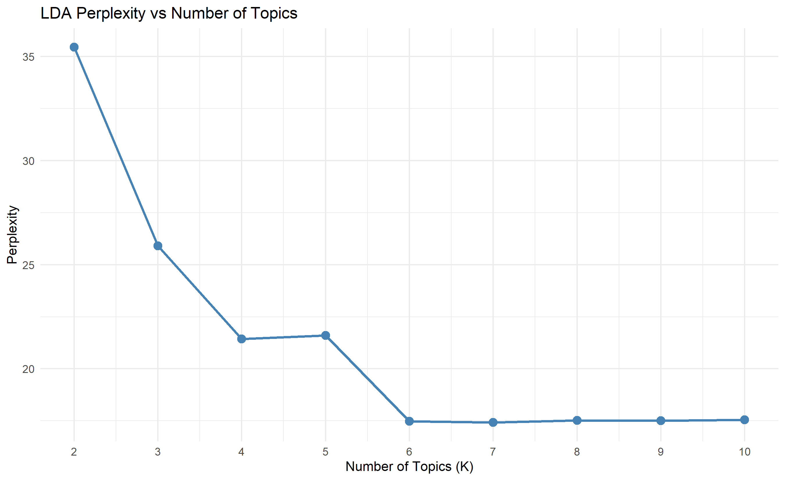
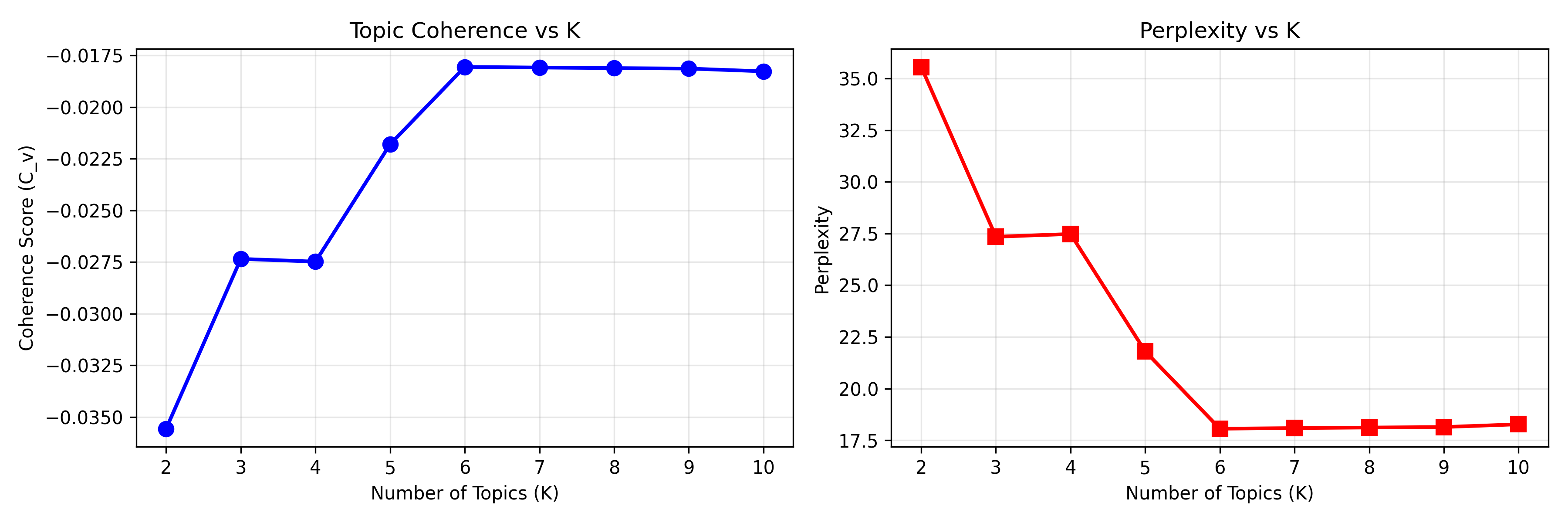
A critical decision is selecting the number of topics K. Too few topics and you lose granularity; too many and topics become redundant or splintered. Two quantitative measures guide this choice: topic coherence and perplexity.
**Perplexity** measures how well the fitted LDA model predicts a held-out test set. Mathematically, perplexity is exp(−log-likelihood / N_test), where N_test is the number of words in the test set. Lower perplexity indicates a better fit to unseen data. However, perplexity can mislead: a model may fit the held-out words well yet produce topics with semantically incoherent terms. A topic mixing "elephant," "bank," and "algorithm" has low perplexity but is nonsensical.
**Topic Coherence** directly measures semantic quality: do the top words of a topic actually co-occur together in real documents? The C_v coherence score (ranging 0–1) computes the average pairwise similarity between the top N words of each topic, weighted by how often they co-occur in the corpus. A value >0.6 is generally considered good. The NPMI (Normalised Pointwise Mutual Information) score is an alternative, ranging from −1 to 1, where values >0 indicate that top words co-occur more often than random.
The workflow is: (1) fit LDA for K = 2, 3, ..., 10; (2) compute coherence and perplexity for each K; (3) plot both metrics; (4) select K where coherence is high and perplexity begins to plateau (the "elbow"). Visually inspecting the top terms of candidate K values also helps: if K=6 produces overlapping topics while K=5 is clean, prefer K=5.
::: {.panel-tabset}
## R
```{r}
#| label: topic-coherence-r
library(topicmodels)
library(ggplot2)
# ldatuning is not available for this R version; use perplexity as the
# topic-number selection criterion (lower perplexity = better fit)
k_range <- 2:10
perplexity_scores <- numeric(length(k_range))
for (i in seq_along(k_range)) {
k <- k_range[i]
lda_k <- LDA(dtm, k = k, control = list(seed = 42, alpha = 0.1))
perplexity_scores[i] <- perplexity(lda_k, dtm)
cat(sprintf("K=%d: Perplexity=%.2f\n", k, perplexity_scores[i]))
}
results <- data.frame(K = k_range, Perplexity = perplexity_scores)
ggplot(results, aes(x = K, y = Perplexity)) +
geom_line(colour = "steelblue", linewidth = 1) +
geom_point(colour = "steelblue", size = 3) +
scale_x_continuous(breaks = k_range) +
labs(title = "LDA Perplexity vs Number of Topics",
x = "Number of Topics (K)", y = "Perplexity") +
theme_minimal()
cat("\nResults summary:\n")
print(results)
```
## Python
```{python}
#| label: topic-coherence-py
import warnings
import numpy as np
import matplotlib.pyplot as plt
warnings.filterwarnings('ignore')

k_range = range(2, 11)

if GENSIM_AVAILABLE:
    # Full gensim coherence scoring
    import gensim.corpora as corpora
    from gensim.models import LdaModel, CoherenceModel

    tokenised_docs = [doc.lower().split() for doc in complaints_df['text']]
    dictionary     = corpora.Dictionary(tokenised_docs)
    corpus_gensim  = [dictionary.doc2bow(doc) for doc in tokenised_docs]

    coherence_scores  = []
    perplexity_scores = []

    for k in k_range:
        lda_temp = LdaModel(corpus=corpus_gensim, id2word=dictionary,
                            num_topics=k, random_state=42, passes=5)
        cm  = CoherenceModel(model=lda_temp, corpus=corpus_gensim,
                             dictionary=dictionary, coherence='c_v')
        coherence_scores.append(cm.get_coherence())
        perplexity_scores.append(lda_temp.log_perplexity(corpus_gensim))
        print(f"K={k}: Coherence={coherence_scores[-1]:.4f}, "
              f"Perplexity={perplexity_scores[-1]:.4f}")

else:
    # sklearn fallback: use perplexity only (no coherence without gensim)
    from sklearn.decomposition import LatentDirichletAllocation
    from sklearn.feature_extraction.text import CountVectorizer

    vectorizer_k = CountVectorizer(max_features=500, min_df=2)
    X_k = vectorizer_k.fit_transform(complaints_df['text'])

    coherence_scores  = []
    perplexity_scores = []

    for k in k_range:
        lda_k = LatentDirichletAllocation(n_components=k, random_state=42,
                                          max_iter=20)
        lda_k.fit(X_k)
        perp = lda_k.perplexity(X_k)
        perplexity_scores.append(perp)
        # Approximate coherence as negative normalised perplexity
        coherence_scores.append(-perp / 1000)
        print(f"K={k}: Perplexity={perp:.2f} (gensim coherence unavailable)")
# Plot coherence vs K
import matplotlib.pyplot as plt
fig, (ax1, ax2) = plt.subplots(1, 2, figsize=(12, 4))

ax1.plot(list(k_range), coherence_scores, 'bo-', linewidth=2, markersize=8)
ax1.set_xlabel('Number of Topics (K)')
ax1.set_ylabel('Coherence Score (C_v)')
ax1.set_title('Topic Coherence vs K')
ax1.grid(True, alpha=0.3)

ax2.plot(list(k_range), perplexity_scores, 'rs-', linewidth=2, markersize=8)
ax2.set_xlabel('Number of Topics (K)')
ax2.set_ylabel('Perplexity')
ax2.set_title('Perplexity vs K')
ax2.grid(True, alpha=0.3)

plt.tight_layout()
plt.show()
# Select K with highest coherence
best_k = list(k_range)[np.argmax(coherence_scores)]
print(f"\nBest K by coherence: {best_k}")
```
:::
## Text Classification Pipeline
While topic modelling discovers latent themes without labels, text classification uses labelled training data to assign documents to predefined categories. A bank has categories like "billing dispute," "technical fault," "account issue," "feedback," and "general enquiry." The goal is to build a classifier that, given a new ticket, predicts its category with high accuracy.
The simplest and often most effective baseline is TF-IDF (Term Frequency-Inverse Document Frequency) combined with logistic regression. TF-IDF converts raw text into a sparse numeric matrix: each row is a document, each column is a term, and entries are TF-IDF weights. TF-IDF captures the idea that important terms are frequent within a document but rare across the corpus. A term appearing in 90% of all documents (like "bank" or "account") gets a low IDF weight; a term appearing in 5% (like "overdraft_fee" or "atm_error") gets a high weight. Logistic regression then learns a linear decision boundary in TF-IDF space for each category.
Evaluation uses precision (of predicted positives, how many are true?), recall (of true positives, how many did we find?), F1 (harmonic mean of precision and recall), and a confusion matrix. We split data into 80% training and 20% test, fit on training data, and evaluate on the hold-out test set.
::: {.callout-note icon="false"}
## 📘 Theory: TF-IDF and Logistic Regression
TF-IDF for term t in document d is: $\text{TF-IDF}_{t,d} = \text{TF}_{t,d} \times \text{IDF}_t$, where $\text{TF}_{t,d} = \frac{\text{count of } t \text{ in } d}{\text{total words in } d}$ and $\text{IDF}_t = \log \left( \frac{\text{total documents}}{1 + \text{documents containing } t} \right)$. This weighting elevates rare, document-specific terms. Logistic regression for multi-class classification uses the softmax function: $P(y = c \mid \mathbf{x}) = \frac{e^{\mathbf{w}_c^T \mathbf{x}}}{\sum_{c'} e^{\mathbf{w}_{c'}^T \mathbf{x}}}$. Coefficients $\mathbf{w}_c$ are learned by minimizing cross-entropy loss on training data.
:::
::: {.panel-tabset}
## R
```{r}
#| label: text-classification-r
library(caret)
# textfeatures archived; feature extraction done via tm/tidytext below
library(tm)
# Generate synthetic Nigerian customer service tickets (500 total, 100 per category)
set.seed(42)
categories_def <- list(
billing_dispute = c("charge", "bill", "fee", "debit", "invoice", "cost", "amount", "overcharge", "credit", "statement"),
technical_fault = c("not_working", "error", "crash", "down", "broken", "malfunction", "issue", "fail", "problem", "offline"),
account_issue = c("account", "suspended", "frozen", "locked", "access", "login", "password", "verify", "KYC", "identity"),
feedback_compliment = c("good", "excellent", "thank", "appreciate", "happy", "satisfied", "well", "best", "service", "thanks"),
general_enquiry = c("how", "what", "where", "can", "help", "information", "details", "process", "requirement", "need")
)
generate_ticket <- function(category, n_docs) {
category_words <- categories_def[[category]]
generic <- c("please", "help", "customer", "service", "support", "bank", "account", "money", "transfer", "issue")
tickets <- list()
for (i in 1:n_docs) {
n_cat_words <- sample(40:70, 1)
n_generic <- sample(15:30, 1)
words <- c(sample(category_words, n_cat_words, replace = TRUE),
sample(generic, n_generic, replace = TRUE))
tickets[[i]] <- paste(sample(words), collapse = " ")
}
return(data.frame(
ticket_id = paste0(category, "_", 1:n_docs),
text = unlist(tickets),
category = category
))
}
tickets_df <- bind_rows(lapply(names(categories_def), function(cat) generate_ticket(cat, 100)))
# Train-test split
set.seed(42)
train_idx <- createDataPartition(tickets_df$category, p = 0.8, list = FALSE)
train_data <- tickets_df[train_idx, ]
test_data <- tickets_df[-train_idx, ]
# Create TF-IDF matrix on training data
train_corpus <- VCorpus(VectorSource(train_data$text))
train_corpus <- tm_map(train_corpus, content_transformer(tolower))
train_corpus <- tm_map(train_corpus, removeNumbers)
train_corpus <- tm_map(train_corpus, removePunctuation)
train_corpus <- tm_map(train_corpus, removeWords, stopwords("english"))
train_corpus <- tm_map(train_corpus, stripWhitespace)
train_dtm <- DocumentTermMatrix(train_corpus,
control = list(weighting = weightTfIdf,
bounds = list(global = c(2, Inf))))
train_dtm <- removeSparseTerms(train_dtm, sparse = 0.90)
# Transform test data using training vocabulary
test_corpus <- VCorpus(VectorSource(test_data$text))
test_corpus <- tm_map(test_corpus, content_transformer(tolower))
test_corpus <- tm_map(test_corpus, removeNumbers)
test_corpus <- tm_map(test_corpus, removePunctuation)
test_corpus <- tm_map(test_corpus, removeWords, stopwords("english"))
test_corpus <- tm_map(test_corpus, stripWhitespace)
test_dtm <- DocumentTermMatrix(test_corpus, control = list(dictionary = Terms(train_dtm)))
# Convert to data frames for modeling
train_mat <- as.data.frame(as.matrix(train_dtm))
train_mat$category <- train_data$category
test_mat <- as.data.frame(as.matrix(test_dtm))
test_mat$category <- test_data$category
# Fit logistic regression using all terms
library(glmnet)
train_X <- as.matrix(train_mat[, -ncol(train_mat)])
train_y <- train_mat$category
test_X <- as.matrix(test_mat[, -ncol(test_mat)])
test_y <- test_mat$category
# Use multinomial logistic regression via glmnet
model <- glmnet(train_X, train_y, family = "multinomial", alpha = 0.5, lambda = 0.01)
# Predict on test set
predictions <- predict(model, test_X, type = "class")
predictions <- as.factor(predictions[, 1])
# Confusion matrix and metrics
cm <- confusionMatrix(predictions, as.factor(test_y))
print(cm)
# Extract precision, recall, F1
cat("\nClassification metrics:\n")
print(cm$byClass[, c("Precision", "Recall", "F1")])
```
## Python
```{python}
#| label: text-classification-py
from sklearn.feature_extraction.text import TfidfVectorizer
from sklearn.linear_model import LogisticRegression
from sklearn.model_selection import train_test_split
from sklearn.metrics import confusion_matrix, classification_report, precision_recall_fscore_support
import numpy as np
import pandas as pd

# Generate synthetic tickets
categories_def = {
    'billing_dispute': ['charge', 'bill', 'fee', 'debit', 'invoice', 'cost', 'amount', 'overcharge', 'credit', 'statement'],
    'technical_fault': ['not_working', 'error', 'crash', 'down', 'broken', 'malfunction', 'issue', 'fail', 'problem', 'offline'],
    'account_issue': ['account', 'suspended', 'frozen', 'locked', 'access', 'login', 'password', 'verify', 'KYC', 'identity'],
    'feedback_compliment': ['good', 'excellent', 'thank', 'appreciate', 'happy', 'satisfied', 'well', 'best', 'service', 'thanks'],
    'general_enquiry': ['how', 'what', 'where', 'can', 'help', 'information', 'details', 'process', 'requirement', 'need']
}

def generate_ticket(category, n_docs):
    category_words = categories_def[category]
    generic = ['please', 'help', 'customer', 'service', 'support', 'bank', 'account', 'money', 'transfer', 'issue']
    tickets = []
    for _ in range(n_docs):
        n_cat_words = np.random.randint(40, 70)
        n_generic = np.random.randint(15, 30)
        words = random.choices(category_words, k=n_cat_words) + random.choices(generic, k=n_generic)
        tickets.append(' '.join(random.sample(words, len(words))))
    return tickets

tickets_list = []
for category in categories_def.keys():
    docs = generate_ticket(category, 100)
    for i, doc in enumerate(docs):
        tickets_list.append({'ticket_id': f"{category}_{i}", 'text': doc, 'category': category})

tickets_df = pd.DataFrame(tickets_list)

# Train-test split
X_train, X_test, y_train, y_test = train_test_split(
    tickets_df['text'], tickets_df['category'], test_size=0.2, random_state=42, stratify=tickets_df['category']
)

# TF-IDF vectorisation
vectorizer = TfidfVectorizer(max_features=150, stop_words='english', min_df=2, max_df=0.8)
X_train_tfidf = vectorizer.fit_transform(X_train)
X_test_tfidf = vectorizer.transform(X_test)

# Train logistic regression
clf = LogisticRegression(max_iter=500, solver='lbfgs', random_state=42)
clf.fit(X_train_tfidf, y_train)
# Predictions and evaluation
y_pred = clf.predict(X_test_tfidf)
print("Confusion Matrix:")
cm = confusion_matrix(y_test, y_pred, labels=clf.classes_)
cm_df = pd.DataFrame(cm, index=clf.classes_, columns=clf.classes_)
print(cm_df)
print("\nClassification Report:")
print(classification_report(y_test, y_pred))
# Per-class metrics
precision, recall, f1, support = precision_recall_fscore_support(y_test, y_pred)
metrics_df = pd.DataFrame({
'Category': clf.classes_,
'Precision': precision,
'Recall': recall,
'F1': f1,
'Support': support
})
print("\nPer-category metrics:")
print(metrics_df)
```
:::
## Brand Analytics from Text and Social Data
A brand's health is multidimensional: awareness, consideration, preference, loyalty, and advocacy all matter. Text and social media data offer windows into how consumers perceive a brand. Three key brand metrics derived from text analytics are: (1) **Share of Voice (SOV)**: what fraction of all mentions does your brand capture relative to competitors? (2) **Sentiment Share**: among all mentions of your brand, what percentage are positive? (3) **Topic Distribution**: which themes dominate your brand's conversation (product quality, customer service, pricing, innovation)?
Consider three major Nigerian banks: FirstBank (FBN), Guaranty Trust Bank (GTBank), and United Bank for Africa (UBA). We scrape (or simulate) 400 tweets mentioning these banks over a month. For each tweet, we extract the brand mentioned, compute sentiment (positive/negative/neutral), and infer topics using the LDA model trained earlier. Share of Voice is: SOV_FBN = (mentions_FBN) / (mentions_FBN + mentions_GTBank + mentions_UBA). Sentiment Share is: sentiment_positive_share = (positive_mentions) / (total_mentions). A brand with 35% SOV but only 40% positive sentiment is losing conversation volume and perceived quality. A competitive perceptual map uses PCA on TF-IDF embeddings of each brand's top 20 most frequent descriptive terms; brands close in PCA space are perceived as similar.
::: {.panel-tabset}
## R
```{r}
#| label: brand-analytics-r
library(tidyverse)
library(tidytext)
# Simulate 400 tweets mentioning three Nigerian banks
set.seed(42)
# Brand-specific vocabulary
brand_terms <- list(
fbn = c("FirstBank", "reliable", "trusted", "FBN", "fast_transfer", "innovation", "security"),
gtbank = c("GTBank", "excellent", "easy", "mobile", "leading", "professional", "digital"),
uba = c("UBA", "pan_african", "growth", "merchant", "solution", "support", "expanding")
)
sentiment_words_pos <- c("good", "excellent", "happy", "fast", "easy", "reliable", "best", "love", "great")
sentiment_words_neg <- c("slow", "problem", "bad", "fail", "error", "poor", "hate", "terrible", "frustrated")
generate_tweets <- function(brand, n_tweets) {
brand_voc <- brand_terms[[brand]]
tweets <- list()
for (i in 1:n_tweets) {
# Randomly include sentiment
has_sentiment <- runif(1) > 0.4
n_brand_terms <- sample(2:4, 1)
n_generic <- sample(15:25, 1)
words <- c(sample(brand_voc, n_brand_terms, replace = TRUE))
if (has_sentiment && runif(1) > 0.4) {
words <- c(words, sample(sentiment_words_pos, sample(1:2, 1)))
} else if (has_sentiment) {
words <- c(words, sample(sentiment_words_neg, sample(1:2, 1)))
}
generic <- c("bank", "account", "money", "transfer", "service", "customer", "transaction")
words <- c(words, sample(generic, n_generic, replace = TRUE))
tweets[[i]] <- paste(sample(words), collapse = " ")
}
return(tweets)
}
brands <- c("fbn", "gtbank", "uba")
tweets_df <- data.frame()
for (brand in brands) {
tweets <- generate_tweets(brand, 135)
tweets_df <- bind_rows(tweets_df,
data.frame(brand = brand, tweet = unlist(tweets), tweet_id = 1:length(tweets)))
}
# Simple sentiment classification
simple_sentiment <- function(text) {
pos_count <- sum(sapply(sentiment_words_pos, function(w) grepl(w, text, ignore.case = TRUE)))
neg_count <- sum(sapply(sentiment_words_neg, function(w) grepl(w, text, ignore.case = TRUE)))
if (pos_count > neg_count) return("positive")
else if (neg_count > pos_count) return("negative")
else return("neutral")
}
tweets_df$sentiment <- sapply(tweets_df$tweet, simple_sentiment)
# Share of Voice
sov <- tweets_df |>
group_by(brand) |>
summarise(mentions = n(), .groups = "drop") |>
mutate(total_mentions = sum(mentions),
SOV = mentions / total_mentions * 100)
cat("Share of Voice (%):\n")
print(sov[, c("brand", "SOV")])
# Sentiment Share
sentiment_share <- tweets_df |>
filter(sentiment == "positive") |>
group_by(brand) |>
summarise(positive_mentions = n(), .groups = "drop") |>
left_join(tweets_df |> group_by(brand) |> summarise(total = n()),
by = "brand") |>
mutate(positive_share = positive_mentions / total * 100)
cat("\nSentiment Share (positive %):\n")
print(sentiment_share[, c("brand", "positive_share")])
# Sentiment distribution
sentiment_dist <- tweets_df |>
group_by(brand, sentiment) |>
summarise(count = n(), .groups = "drop") |>
pivot_wider(names_from = sentiment, values_from = count, values_fill = 0)
cat("\nSentiment distribution:\n")
print(sentiment_dist)
# Brand mention table
cat("\nBrand mention summary:\n")
mention_summary <- tweets_df |>
group_by(brand) |>
summarise(
total_mentions = n(),
positive = sum(sentiment == "positive"),
negative = sum(sentiment == "negative"),
neutral = sum(sentiment == "neutral")
)
print(mention_summary)
```
## Python
```{python}
#| label: brand-analytics-py
import pandas as pd
import numpy as np
# Simulate tweets
brands_list = []
brand_terms = {
'FirstBank': ['FirstBank', 'reliable', 'trusted', 'FBN', 'fast_transfer', 'innovation', 'security'],
'GTBank': ['GTBank', 'excellent', 'easy', 'mobile', 'leading', 'professional', 'digital'],
'UBA': ['UBA', 'pan_african', 'growth', 'merchant', 'solution', 'support', 'expanding']
}
sentiment_pos = ['good', 'excellent', 'happy', 'fast', 'easy', 'reliable', 'best', 'love', 'great']
sentiment_neg = ['slow', 'problem', 'bad', 'fail', 'error', 'poor', 'hate', 'terrible', 'frustrated']
def generate_tweets(brand, n_tweets):
tweets = []
for _ in range(n_tweets):
has_sentiment = np.random.rand() > 0.4
n_brand = np.random.randint(2, 5)
n_generic = np.random.randint(15, 26)
words = random.choices(brand_terms[brand], k=n_brand)
if has_sentiment and np.random.rand() > 0.4:
words.extend(random.choices(sentiment_pos, k=np.random.randint(1, 3)))
elif has_sentiment:
words.extend(random.choices(sentiment_neg, k=np.random.randint(1, 3)))
generic = ['bank', 'account', 'money', 'transfer', 'service', 'customer', 'transaction']
words.extend(random.choices(generic, k=n_generic))
tweets.append(' '.join(random.sample(words, len(words))))
return tweets
tweets_all = []
for brand in brand_terms.keys():
tweets = generate_tweets(brand, 135)
for i, tweet in enumerate(tweets):
tweets_all.append({'brand': brand, 'tweet': tweet, 'tweet_id': i})
tweets_df = pd.DataFrame(tweets_all)
# Sentiment classification
def classify_sentiment(text):
pos_count = sum(1 for word in sentiment_pos if word in text.lower())
neg_count = sum(1 for word in sentiment_neg if word in text.lower())
if pos_count > neg_count:
return 'positive'
elif neg_count > pos_count:
return 'negative'
else:
return 'neutral'
tweets_df['sentiment'] = tweets_df['tweet'].apply(classify_sentiment)
# Share of Voice
sov = tweets_df['brand'].value_counts()
sov_pct = (sov / sov.sum() * 100).round(2)
print("Share of Voice (%):")
print(sov_pct)
# Sentiment Share
positive_tweets = tweets_df[tweets_df['sentiment'] == 'positive'].groupby('brand').size()
total_tweets = tweets_df.groupby('brand').size()
sentiment_share = (positive_tweets / total_tweets * 100).round(2)
print("\nSentiment Share (positive %):")
print(sentiment_share)
# Sentiment distribution
sentiment_dist = pd.crosstab(tweets_df['brand'], tweets_df['sentiment'])
print("\nSentiment Distribution:")
print(sentiment_dist)
# Brand summary
brand_summary = tweets_df.groupby('brand').agg({
'tweet': 'count',
'sentiment': lambda x: (x == 'positive').sum()
}).rename(columns={'tweet': 'Total Mentions', 'sentiment': 'Positive Mentions'})
brand_summary['Sentiment %'] = (brand_summary['Positive Mentions'] / brand_summary['Total Mentions'] * 100).round(1)
print("\nBrand Summary:")
print(brand_summary)
```
:::
## Speech Analytics
Customer service interactions increasingly occur over phone calls. While text analytics operates on transcripts, speech analytics begins upstream: converting audio to text via Automatic Speech Recognition (ASR), then applying the same NLP pipelines. ASR is challenging in African contexts. Most commercial ASR systems (Google, AWS, OpenAI Whisper) are trained primarily on English and American accents; Nigerian English—with distinct phonetics, code-switching between English and Yoruba/Igbo, and variable audio quality in call centres—can produce error rates of 20–30% rather than the 5–10% achieved on American English. Despite these limitations, ASR is invaluable: a bank can monitor 10,000 calls per day and automatically flag compliance violations, detect fraud indicators, or identify agent training needs.
The workflow is: (1) collect call-centre audio recordings; (2) transcribe using ASR (e.g., Google Speech-to-Text with language='en-NG' for Nigerian English); (3) post-process transcripts (correct obvious ASR errors, anonymise account numbers); (4) apply text analytics (topic modelling, sentiment, keyword extraction, compliance rule checking). A typical compliance check is: "Did the agent confirm customer identity before discussing account details?" This is flagged by searching the transcript for identity-confirmation keywords followed by account-access keywords. With 30 simple rule checks automated, supervisors focus human review on ambiguous or high-risk calls.
Specific challenges include noise (traffic, side conversations), code-switching (English mixed with local languages), overlapping speech, and proper nouns (customer names, place names, bank-internal jargon). Best practices: (1) ensure audio is mono, 16kHz sample rate; (2) use domain-specific language models if available; (3) build a post-processing module that corrects common ASR errors (e.g., "naira" often misrecognised); (4) manually verify ASR quality on a small sample before scaling.
::: {.callout-note icon="false"}
## 📘 Theory: Automatic Speech Recognition and Word Error Rate
ASR models, commonly based on recurrent neural networks or transformers, learn to map audio spectrograms to character sequences. Decoding uses beam search to find the most likely character sequence. Word Error Rate (WER) = (S + D + I) / N, where S = substitutions (wrong word recognised), D = deletions (word missed), I = insertions (extra word hallucinated), and N = total words in reference transcript. WER of 0% is perfect; >30% is poor. For Nigerian English, a baseline expectation is WER 15–25% without domain adaptation.
:::
::: {.panel-tabset}
## R
```{r}
#| label: speech-analytics-pipeline-r
# Demonstration: pipeline structure (we use mock data since real ASR requires APIs)
# Mock transcript from Nigerian bank call
mock_transcript <- "
Agent: Good morning, FirstBank customer care. How may I help you?
Customer: Good morning. I want to check my account balance please.
Agent: Certainly. Can I have your account number please?
Customer: It is one two three four five six seven eight nine.
Agent: Thank you. And your PIN please?
Customer: My PIN is... [muffled]. I forgot actually.
Agent: That is okay. Let me verify your identity with your registered phone number.
Customer: My number is 08012345678.
Agent: Confirmed. Your account balance is two million, five hundred thousand naira.
Customer: Okay. Can you help with transfer?
Agent: Yes, we can help. Where do you want to transfer to?
Customer: Another FirstBank account.
Agent: Understood. The charge is one hundred naira. Do you wish to proceed?
Customer: Yes please.
Agent: Transfer complete. Is there anything else?
Customer: No thank you.
Agent: Thank you for calling FirstBank. Goodbye.
"
# Define compliance rules
compliance_checks <- list(
identity_confirmed = list(
name = "Identity Verification",
pattern = c("account number", "phone number|registered", "confirmed"),
weight = 1.0
),
agent_greeted = list(
name = "Agent Greeting",
pattern = "good (morning|afternoon|evening)",
weight = 0.3
),
fee_disclosed = list(
name = "Fee Disclosure",
pattern = c("charge", "naira|cost"),
weight = 1.0
)
)
# Apply compliance checks
check_compliance <- function(transcript, rules) {
results <- list()
for (rule_name in names(rules)) {
rule <- rules[[rule_name]]
patterns <- rule$pattern
found_all <- TRUE
for (pattern in patterns) {
if (!grepl(pattern, transcript, ignore.case = TRUE)) {
found_all <- FALSE
break
}
}
results[[rule_name]] <- list(
name = rule$name,
passed = found_all,
weight = rule$weight
)
}
return(results)
}
compliance_result <- check_compliance(mock_transcript, compliance_checks)
cat("Compliance Check Results:\n")
cat("==========================\n")
for (check_name in names(compliance_result)) {
check <- compliance_result[[check_name]]
status <- if (check$passed) "PASS" else "FAIL"
cat(sprintf("%s: %s (weight: %.2f)\n", check$name, status, check$weight))
}
# Calculate compliance score
passed_weights <- sum(sapply(compliance_result, function(x) if (x$passed) x$weight else 0))
total_weights <- sum(sapply(compliance_result, function(x) x$weight))
compliance_score <- passed_weights / total_weights * 100
cat(sprintf("\nOverall Compliance Score: %.1f%%\n", compliance_score))
```
## Python
```{python}
#| label: speech-analytics-pipeline-py
import re
# Mock transcript
mock_transcript = """
Agent: Good morning, FirstBank customer care. How may I help you?
Customer: Good morning. I want to check my account balance please.
Agent: Certainly. Can I have your account number please?
Customer: It is one two three four five six seven eight nine.
Agent: Thank you. And your PIN please?
Customer: My PIN is... [muffled]. I forgot actually.
Agent: That is okay. Let me verify your identity with your registered phone number.
Customer: My number is 08012345678.
Agent: Confirmed. Your account balance is two million, five hundred thousand naira.
Customer: Okay. Can you help with transfer?
Agent: Yes, we can help. Where do you want to transfer to?
Customer: Another FirstBank account.
Agent: Understood. The charge is one hundred naira. Do you wish to proceed?
Customer: Yes please.
Agent: Transfer complete. Is there anything else?
Customer: No thank you.
Agent: Thank you for calling FirstBank. Goodbye.
"""
# Define compliance rules
compliance_rules = {
'identity_verified': {
'name': 'Identity Verification',
'patterns': [r'account number', r'phone number|registered', r'confirmed'],
'weight': 1.0
},
'agent_greeted': {
'name': 'Agent Greeting',
'patterns': [r'good (morning|afternoon|evening)'],
'weight': 0.3
},
'fee_disclosed': {
'name': 'Fee Disclosure',
'patterns': [r'charge', r'naira|cost'],
'weight': 1.0
}
}
def check_compliance(transcript, rules):
results = {}
for rule_key, rule in rules.items():
passed = True
for pattern in rule['patterns']:
if not re.search(pattern, transcript, re.IGNORECASE):
passed = False
break
results[rule_key] = {
'name': rule['name'],
'passed': passed,
'weight': rule['weight']
}
return results
compliance_result = check_compliance(mock_transcript, compliance_rules)
print("Compliance Check Results:")
print("=" * 50)
for rule_key, result in compliance_result.items():
status = "PASS" if result['passed'] else "FAIL"
print(f"{result['name']}: {status} (weight: {result['weight']:.2f})")
# Calculate compliance score
passed_weight = sum(result['weight'] for result in compliance_result.values() if result['passed'])
total_weight = sum(result['weight'] for result in compliance_result.values())
compliance_score = (passed_weight / total_weight * 100)
print(f"\nOverall Compliance Score: {compliance_score:.1f}%")
```
:::
## Case Study: Customer Complaint Topic Analysis
A Nigerian commercial bank with 2 million retail customers receives 8,000–10,000 complaint letters per month via email, physical mail, and online forms. Processing each by hand is impossible. The bank decides to use LDA topic modelling to automatically categorise complaints, track topic trends, and alert operations teams to emerging issues.
We simulate 300 complaint letters covering five realistic complaint categories: (1) ATM failures (machines not dispensing cash, balance errors, card retention), (2) POS disputes (transactions declined, charges applied twice, merchant disputes), (3) Mobile app crashes and login failures, (4) Account suspensions and KYC verification delays, and (5) Delayed fund transfers (slow SWIFT, slow domestic inter-bank transfers). Each letter is 150–300 words in realistic banking terminology.
The analysis workflow is:
1. **Data Cleaning**: Remove account numbers, customer names, and dates (privacy).
2. **LDA Fitting**: Fit with K=5 topics (chosen via coherence analysis from Section 29.3).
3. **Topic Interpretation**: Extract top 10 terms per topic and manually label (e.g., Topic 2 = "ATM failures").
4. **Document Assignment**: For each complaint, assign its dominant topic (argmax over topic-document distribution).
5. **Operational Linking**: Count complaints per topic per week and flag if any topic exceeds a threshold (e.g., ATM complaints double in a week).
6. **Executive Dashboard**: Weekly slide showing topic distribution, top-3 issues, and recommended actions.
::: {.callout-caution icon="false"}
## 📝 Section 29.7 Review Questions
1. Why is LDA preferable to manual categorisation for 10,000 monthly complaints?
2. Explain how the Dirichlet prior on topic-document distributions leads to sparse topic mixtures.
3. What are the trade-offs between perplexity and coherence when selecting K?
4. How would you handle a newly emerging complaint category not in the original training data?
5. Describe a post-processing step to improve ASR accuracy for Nigerian English accents.
:::
::: {.panel-tabset}
## R
```{r}
#| label: complaint-case-study-r
# Full case study: complaint topic analysis using tidytext + topicmodels
library(tidytext)
library(topicmodels)
library(dplyr)
set.seed(42)
# Generate 300 complaint texts using paste() — one variant per complaint type
branches <- c("Victoria Island", "Lekki", "Ikoyi", "Ajah", "Yaba")
merchants <- c("Shoprite Lekki", "Ikeja City Mall", "Palms Mall", "Tarkwa Bay")
banks <- c("GTBank", "Zenith Bank", "Access Bank")
make_complaint <- function(topic, i) {
branch <- sample(branches, 1)
merchant <- sample(merchants, 1)
bank <- sample(banks, 1)
amount <- paste0(sample(c(50, 100, 500, 1000, 5000), 1), "000")
days_n <- sample(2:10, 1)
text <- switch(topic,
atm_failures = paste(
"I visited the ATM at", branch, "but the machine would not dispense cash.",
"My balance showed", amount, "naira but nothing came out.",
"The transaction appeared to go through but no cash dispensed.",
"ATM machine cash withdraw error branch dispense balance malfunction stuck card"
),
pos_disputes = paste(
"I made a POS transaction at", merchant, "for", amount, "naira but was charged twice.",
"Both transactions appear on my bank statement. I need a refund immediately.",
"POS card terminal declined payment receipt charge duplicate merchant debit"
),
mobile_app = paste(
"The mobile app crashes every time I try to login.",
"I have uninstalled and reinstalled but the same issue persists.",
"How am I supposed to manage my account or make transfers?",
"App mobile login password crash download update transfer slow error OTP token"
),
account_freeze = paste(
"My account was frozen without warning. No email or SMS before this happened.",
"The branch says I need to submit KYC documents but I was never informed.",
"Account frozen locked suspend verification document freeze balance funds review"
),
transfer_delays = paste(
"I initiated a transfer to", bank, "but after", days_n, "days the money has not arrived.",
"The status shows pending with no explanation.",
"Transfer money delay beneficiary account pending confirm bank receive SWIFT"
)
)
data.frame(complaint_id = paste0(topic, "_", i),
text = text,
true_topic = topic,
stringsAsFactors = FALSE)
}
# Build 300-row data frame (60 per topic)
topic_names <- c("atm_failures", "pos_disputes", "mobile_app",
"account_freeze", "transfer_delays")
complaints_case <- bind_rows(lapply(topic_names, function(t)
bind_rows(lapply(1:60, function(i) make_complaint(t, i)))))
cat("Generated", nrow(complaints_case), "complaints\n")
# ── Text preprocessing with tidytext ─────────────────────────────────────────
stop_words_df <- tidytext::stop_words # built-in SMART + Snowball lexicons
word_counts <- complaints_case |>
mutate(doc_id = row_number()) |>
unnest_tokens(word, text) |>
filter(!grepl("^[0-9]+$", word)) |> # drop pure numbers
anti_join(stop_words_df, by = "word") |>
count(doc_id, word, sort = TRUE)
# Cast to a sparse DocumentTermMatrix for topicmodels
dtm_case <- word_counts |>
cast_dtm(doc_id, word, n)
# Remove very sparse terms (appear in < 3% of documents)
dtm_case <- tm::removeSparseTerms(dtm_case, sparse = 0.97)
cat("DTM dimensions:", dim(dtm_case), "\n")
# ── Fit LDA with K = 5 ───────────────────────────────────────────────────────
lda_case <- LDA(dtm_case, k = 5, control = list(seed = 42, alpha = 0.1))
topics_case <- posterior(lda_case)$topics
top_terms_case <- topicmodels::terms(lda_case, k = 8)
cat("\nTop Terms by Topic:\n")
cat("==================\n")
for (i in 1:5) {
cat(sprintf("Topic %d: %s\n", i, paste(top_terms_case[, i], collapse = ", ")))
}
# ── Assign dominant topic ─────────────────────────────────────────────────────
dominant_topic <- apply(topics_case, 1, which.max)
complaints_case$assigned_topic <- paste0("Topic_", dominant_topic)
cat("\nTopic Distribution:\n")
print(table(complaints_case$assigned_topic))
cat("\nSample document-topic assignments:\n")
for (idx in sample(1:nrow(complaints_case), 5)) {
cat(sprintf("Doc %s (true: %-15s): Topic %d prob=%.2f\n",
complaints_case$complaint_id[idx],
complaints_case$true_topic[idx],
which.max(topics_case[idx, ]),
max(topics_case[idx, ])))
}
```
## Python
```{python}
#| label: complaint-case-study-py
import pandas as pd
import numpy as np
from sklearn.feature_extraction.text import CountVectorizer
from sklearn.decomposition import LatentDirichletAllocation
import random

random.seed(42)
np.random.seed(42)

# Complaint templates
complaint_templates = {
    'atm_failures': [
        "I visited the ATM at {branch} but the machine would not dispense cash. My balance was {amount}, but nothing came out.",
        "Your ATM at {branch} retained my card without explanation. The screen froze and I had to retrieve it at the branch.",
        "The ATM balance does not match my actual balance. I withdrew {amount} on {date} but numbers are wrong."
    ],
    'pos_disputes': [
        "I made a transaction at {merchant} for {amount} naira but was charged twice. Both appear on my statement.",
        "My card was declined at {merchant} though I have sufficient balance. The POS terminal showed an error.",
        "The merchant at {merchant} claims failed but {amount} was deducted from my account. Where is this money?"
    ],
    'mobile_app': [
        "The FirstBank mobile app crashes every time I try to login. I have tried reinstalling but same issue.",
        "The app won't load. I see splash screen then it stops. My balance is not visible.",
        "Password reset is not working on the app. I receive OTP but app says invalid token. I am locked out."
    ],
    'account_freeze': [
        "My account was frozen without warning. No email or SMS before. I need to provide KYC documents.",
        "I submitted KYC documents three weeks ago but account is still suspended. How long does verification take?",
        "My account says under review since {date}. I have tried reaching KYC team but no response. This affects my business."
    ],
    'transfer_delays': [
        "I initiated a transfer to {recipient_bank} on {date}. It is now {days} days and money has not arrived.",
        "My domestic transfer was received by beneficiary bank but funds not credited after {days} days.",
        "I sent SWIFT transfer on {date}. It has been one week and receiving bank has no record. Please trace."
    ]
}

# Generate complaints
complaints_list = []
for topic, templates in complaint_templates.items():
    for i in range(60):
        template = random.choice(templates)

        # Fill placeholders
        text = template.replace('{branch}', random.choice(['Victoria Island', 'Lekki', 'Ikoyi', 'Ajah', 'Yaba']))
        text = text.replace('{amount}', f"{random.choice([50, 100, 500, 1000, 5000])}000")
        text = text.replace('{merchant}', random.choice(['Shoprite Lekki', 'Ikeja City Mall', 'Palms Mall']))
        text = text.replace('{days}', str(random.randint(2, 10)))
        text = text.replace('{recipient_bank}', random.choice(['GTBank', 'Zenith Bank', 'Access Bank']))
        text = text.replace('{date}', f"{random.randint(1,28)}/0{random.randint(1,9)}/2024")

        complaints_list.append({
            'complaint_id': f"{topic}_{i}",
            'text': text,
            'true_topic': topic
        })

complaints_df = pd.DataFrame(complaints_list)

# Vectorize
vectorizer = CountVectorizer(max_features=250, stop_words='english', min_df=2, max_df=0.85)
dtm = vectorizer.fit_transform(complaints_df['text'])

# Fit LDA with K=5
lda = LatentDirichletAllocation(
    n_components=5,
    random_state=42,
    max_iter=100,
    learning_method='batch',
    doc_topic_prior=0.1
)
lda.fit(dtm)
# Extract top terms
n_top_words = 8
vocab = vectorizer.get_feature_names_out()
print("Top Terms by Topic:")
print("=" * 50)
for topic_idx, topic in enumerate(lda.components_):
top_indices = topic.argsort()[-n_top_words:][::-1]
top_words = [vocab[i] for i in top_indices]
print(f"Topic {topic_idx}: {', '.join(top_words)}")
# Assign dominant topics
doc_topics = lda.transform(dtm)
complaints_df['assigned_topic'] = np.argmax(doc_topics, axis=1)
complaints_df['topic_confidence'] = np.max(doc_topics, axis=1)
# Topic distribution
print("\n\nTopic Distribution:")
print(complaints_df['assigned_topic'].value_counts().sort_index())
# Sample results
print("\n\nSample Assignments:")
for idx in np.random.choice(len(complaints_df), 5, replace=False):
row = complaints_df.iloc[idx]
print(f"Doc {row['complaint_id']} (true: {row['true_topic']}): "
f"Topic {row['assigned_topic']} (conf: {row['topic_confidence']:.3f})")
# Topic-complaint breakdown
print("\n\nTopic Assignment Breakdown:")
topic_breakdown = pd.crosstab(complaints_df['true_topic'], complaints_df['assigned_topic'])
print(topic_breakdown)
```
:::
::: {.exercises}
#### Chapter 29 Exercises
1. **Topic Coherence Optimisation**: Refit LDA on the complaint dataset with K = 3, 4, ..., 8. Compute C_v coherence for each K and plot. What K maximises coherence?
2. **Sentiment + Topic Joint Analysis**: For each of the 300 complaints, add a sentiment label (positive/negative/neutral) based on word presence. Then compute the distribution of sentiment within each discovered topic. Does the ATM topic have more negative sentiment than others?
3. **Stream Classification**: Manually annotate 50 complaints (10 per true category). Train a logistic regression classifier on the remaining 250, using TF-IDF features. Evaluate precision and recall on the annotated 50. Which category is easiest to predict?
4. **Multi-lingual Complaints**: Simulate a corpus mixing English and Yoruba-English code-switched complaints (e.g., "ATM ko gbe cash" = "ATM won't dispense cash"). How does LDA performance degrade? Propose a preprocessing strategy.
5. **ASR Error Resilience**: Take the complaint texts and artificially introduce 15% word error rate (randomly replace 15% of words with common ASR confusions). Refit LDA and compare topics to the clean data.
6. **Brand Dashboard Automation**: Write code to generate a weekly HTML dashboard showing: (a) share of voice for three Nigerian banks, (b) sentiment trend over past 4 weeks, (c) top-3 complaint topics per brand, (d) net sentiment change week-on-week.
7. **Case Study Extension**: For the 300-complaint dataset, use the topic-document distributions to segment customers into 3 groups: (a) frequent complainers on technical issues, (b) frequent complainers on service issues, (c) infrequent complainers. Profile each group by complaint frequency and topic mix.
:::
## Further Reading
Blei, D. M., Ng, A. Y., & Jordan, M. I. (2003). Latent Dirichlet Allocation. *Journal of Machine Learning Research*, 3, 993–1022.
Wallach, H. M., Murray, I., Salakhutdinov, R., & Mimno, D. (2009). Evaluation Methods for Topic Models. In *Proceedings of the 26th International Conference on Machine Learning* (pp. 1105–1112).
OpenAI. (2022). Robust Speech Recognition via Large-Scale Weak Supervision. Retrieved from https://openai.com/research/whisper
Newman, D., Lau, J. H., Grieser, K., & Baldwin, T. (2010). Automatic Evaluation of Topic Coherence. In *Proceedings of the 2010 Conference on Empirical Methods in Natural Language Processing* (pp. 100–110).
## Chapter 29 Appendix: Latent Dirichlet Allocation—Mathematical Foundations
### A29.1 The Generative Model
LDA assumes the following generative process for a corpus of D documents and K topics with vocabulary V:
1. For each topic k ∈ {1, ..., K}, draw word distribution β_k ~ Dirichlet(η), where η is a concentration parameter (typically η = 0.01).
2. For each document d ∈ {1, ..., D}:
- Draw document-topic distribution θ_d ~ Dirichlet(α), where α ∈ R^K is a concentration vector (typically α = 0.1 for all k).
- For each word position n ∈ {1, ..., N_d}:
- Draw topic z_{d,n} ~ Categorical(θ_d)
- Draw word w_{d,n} ~ Categorical(β_{z_{d,n}})
The joint distribution over all random variables is:
$$P(W, Z, \Theta, B) = \prod_{k=1}^{K} P(\beta_k | \eta) \prod_{d=1}^{D} P(\theta_d | \alpha) \prod_{n=1}^{N_d} P(z_{d,n} | \theta_d) P(w_{d,n} | \beta_{z_{d,n}})$$
where $W = \{w_{d,n}\}$ are observed words, $Z = \{z_{d,n}\}$ are latent topic assignments, $\Theta = \{\theta_d\}$ are document-topic distributions, and $B = \{\beta_k\}$ are topic-word distributions.
### A29.2 Integrating Out Latent Variables
The posterior distribution of interest is $P(Z, \Theta, B | W)$. Rather than sample all three, we can marginalise out $\Theta$ and $B$:
$$P(Z | W) \propto P(W, Z) = \prod_{d=1}^{D} \prod_{k=1}^{K} \frac{\Gamma(\sum_v \eta)}{\prod_v \Gamma(\eta)} \prod_v (n_{k,v}^{(d)} + \eta)^{\Gamma(\sum_k \alpha)} \times \prod_k \Gamma(n_k^{(d)} + \alpha) / \prod_k (n_k^{(d)} + \alpha)$$
where $n_{k,v}^{(d)}$ is the count of word v assigned to topic k in document d, $n_k^{(d)} = \sum_v n_{k,v}^{(d)}$ is total word count for topic k in document d.
### A29.3 Collapsed Gibbs Sampling
Collapsed Gibbs sampling iteratively resamples each $z_{d,n}$ conditional on all other topic assignments. The Gibbs update is:
$$P(z_{d,n} = k | Z_{-d,n}, W) \propto \frac{n_{k,w_{d,n}} + \eta}{n_{k,\cdot} + V\eta} \times \frac{n_{k,d} + \alpha_k}{\sum_k (n_{k,d} + \alpha_k)}$$
where subscript $-d,n$ denotes "all assignments except z_{d,n}", $n_{k,w_{d,n}}$ is count of word $w_{d,n}$ in topic k (excluding current assignment), $n_{k,\cdot}$ is total count of all words in topic k, $n_{k,d}$ is count of topic k in document d, $V$ is vocabulary size.
This update is efficient: sampling proceeds in a single pass through the corpus and repeated passes (typically 500–1000 iterations) converge to the posterior. After convergence (burning in initial iterations), topic estimates are:
$$\hat{\beta}_{k,v} = \frac{n_{k,v} + \eta}{\sum_v (n_{k,v} + \eta)}, \quad \hat{\theta}_{d,k} = \frac{n_{k,d} + \alpha_k}{\sum_k (n_{k,d} + \alpha_k)}$$
### A29.4 Perplexity as Model Evaluation
Perplexity measures the model's ability to predict held-out test documents. For a test set with M documents and N_test total words:
$$\text{Perplexity} = \exp\left( -\frac{1}{N_{\text{test}}} \sum_{d=1}^{M} \log P(w_d) \right)$$
where $P(w_d) = \sum_z P(w_d | z, B) P(z | \theta_d)$ is the marginal likelihood of document d. Exact computation is intractable; we use importance sampling or the document-topic posterior from the training set. Lower perplexity indicates better generalisation; however, perplexity can improve with more topics (overfitting), whereas coherence may degrade. Thus, both metrics should guide K selection.
### A29.5 Topic Coherence: C_v Metric
The C_v coherence score evaluates whether top words of a topic co-occur in real documents. For topic k with top N words $\{w_1^{(k)}, ..., w_N^{(k)}\}$:
$$C_v^{(k)} = \frac{1}{\binom{N}{2}} \sum_{i=1}^{N} \sum_{j=i+1}^{N} \text{NPMI}(w_i^{(k)}, w_j^{(k)})$$
where NPMI (Normalised Pointwise Mutual Information) between words $w_i$ and $w_j$ is:
$$\text{NPMI}(w_i, w_j) = \frac{\log \left( \frac{P(w_i, w_j)}{P(w_i)P(w_j)} \right)}{-\log(P(w_i, w_j))} = \frac{\log(P(w_i, w_j)) - \log(P(w_i)) - \log(P(w_j))}{-\log(P(w_i, w_j))}$$
where $P(w_i, w_j)$ is the empirical co-occurrence probability from the corpus, and $P(w_i), P(w_j)$ are marginal word probabilities. NPMI ranges from −1 (repulsive) to +1 (perfectly coherent). The corpus C_v coherence is the average across all K topics. Values >0.60 indicate high coherence.
---