---
title: "Sales Force Analytics"
author: "Bongo Adi"
---
```{python}
#| label: python-setup-47-sales-force-analytics
#| include: false
import numpy as np
import pandas as pd
import matplotlib.pyplot as plt
import seaborn as sns
```
::: {.callout-note icon="false"}
## 📋 Learning Objectives
- Understand the sales funnel as a data system and key pipeline metrics
- Calculate and interpret pipeline health metrics: conversion rates, velocity, coverage ratio
- Perform win/loss analysis and build predictive models for deal outcomes
- Design equitable territories using clustering and workload analysis
- Build regression-based quota setting models
- Analyse sales rep performance with leading and lagging indicators
- Design and simulate incentive compensation plans
- Implement sales force analytics workflows with Nigerian pharmaceutical case study
:::
## The Sales Funnel as a Data System
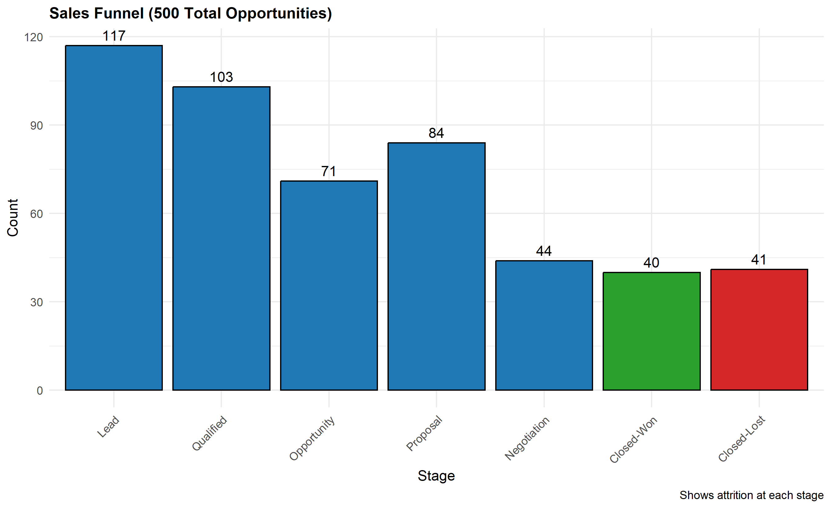
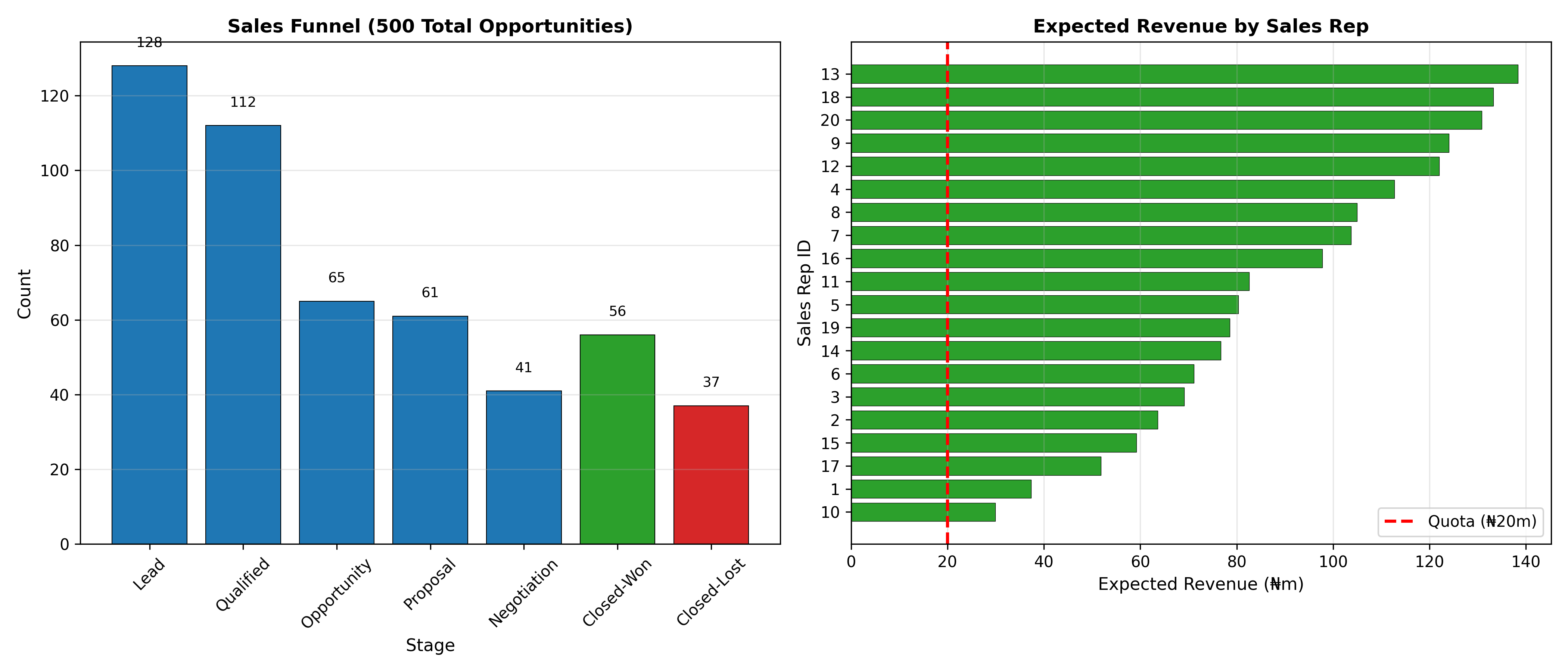
Every step of the sales process generates data. A prospect enters the funnel as a "lead" (a contact, perhaps from a conference, referral, or marketing campaign). The lead is qualified by the sales development representative (SDR): does the prospect fit the ideal customer profile? Qualified leads move into the "opportunity" stage. An opportunity has a deal size (estimated contract value), a sales stage (initial discovery, proposal, negotiation, final approval), and a probability (likelihood of closing). Opportunities mature through stages: the prospect receives a proposal, negotiations occur, objections are addressed, and finally the deal closes (won or lost). Each stage transition is logged in the CRM (Salesforce, HubSpot, MS Dynamics). This data enables measurement and optimization.
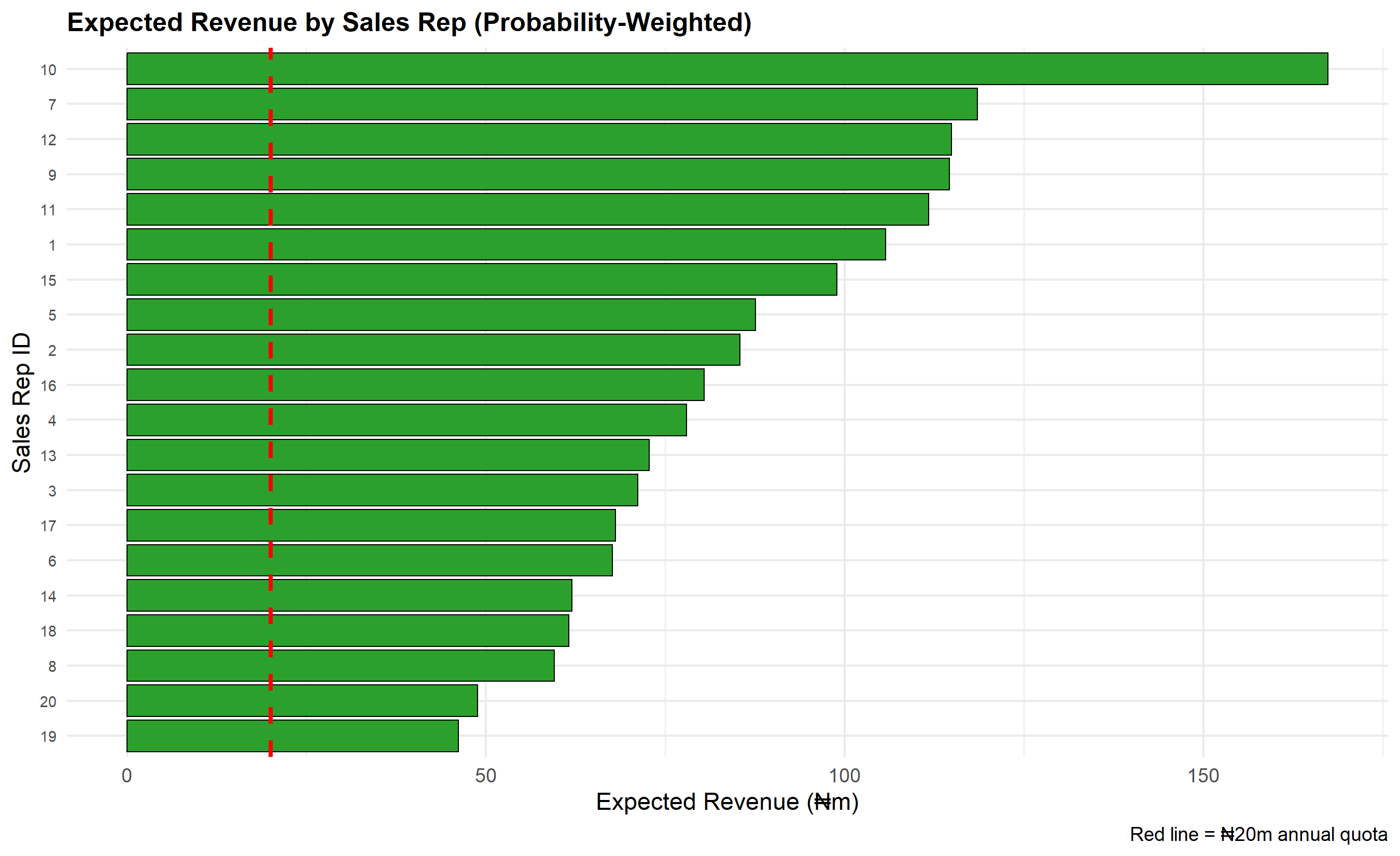
The Nigerian pharmaceutical distribution landscape provides a rich case: representatives call on hospitals, clinics, pharmacies, and wholesalers. Lead sources are diverse—trade conferences (Pharm@Pharma), GP associations, unsolicited walk-ins. Qualification involves assessing hospital bed count (hospital size indicator), annual drug procurement volumes, and existing relationships. The sales cycle is long (2–6 months for hospital contracts) because decisions involve procurement committees. Deal sizes vary from ₦500k (small clinic) to ₦50m (regional hospital network). Pipeline management is critical: a rep with ₦100m in annual quota needs at least ₦250–300m in pipeline (coverage ratio ≥ 2.5x) to absorb normal win rates (30–40%) and pipeline decay.
Key funnel metrics include:
- **Conversion Rate (Stage-to-Stage):** % of leads that advance from one stage to the next. Example: "40% of qualified leads move to proposal stage within 60 days."
- **Sales Cycle Length:** Average time from opportunity creation to close (won or lost). Shorter cycles free capital and rep capacity.
- **Average Deal Size:** Mean contract value per closed deal. Helps quota setting and compensation design.
- **Pipeline Coverage Ratio:** Total pipeline value / annual quota. Rule of thumb: 2.5x+ indicates healthy pipeline.
- **Win Rate:** Percentage of closed opportunities that are won (vs lost). Varies by deal size and stage.
Data quality is critical. Many sales teams under-report lost deals (CRM hygiene issues). A rep might mark a dead opportunity as "on hold" indefinitely. Analytics must flag stale opportunities (no activity for 90+ days) and use CRM audit rules to enforce data integrity.
::: {.callout-note icon="false"}
## 📘 Theory: Pipeline Dynamics and Conversion Funnel
The sales funnel exhibits exponential decay: each stage has a lower count than the previous stage due to attrition. If 100 leads enter, 60 are qualified, 30 become opportunities, 18 move to proposal, 9 to negotiation, and 3 close (won), the conversion rates are: Lead→Qualified = 60%, Qualified→Opportunity = 50%, Opportunity→Proposal = 60%, Proposal→Negotiation = 50%, Negotiation→Closed = 33%. These rates reflect market dynamics and sales effectiveness. Improvement programs (better qualifying, faster proposals) compress the funnel and accelerate revenue generation.
:::
::: {.callout-tip icon="false"}
## 🔑 Key Pipeline Metrics
**Conversion Rate (Stage i to i+1):**
$$\text{Conv}_{i \to i+1} = \frac{\#(\text{Stage } i+1)}{\#(\text{Stage } i)} \times 100\%$$
**Pipeline Coverage:**
$$\text{Coverage Ratio} = \frac{\text{Total Pipeline Value}}{\text{Annual Quota}}$$
**Sales Velocity:**
$$\text{Velocity} = \frac{\text{Opportunities} \times \text{Win Rate} \times \text{Avg Deal Size}}{\text{Sales Cycle Days}} \times 365$$
:::
::: {.panel-tabset}
## R
```{r}
#| label: ch47-pipeline-analytics
#| message: false
#| warning: false
library(tidyverse)
library(ggplot2)
# Synthetic CRM data: 500 opportunities across stages
set.seed(2816)
n_opportunities <- 500
crm_data <- tibble(
Opp_ID = 1:n_opportunities,
Sales_Rep_ID = rep(1:20, length.out = n_opportunities), # 20 reps
Industry = sample(c("Hospital", "Clinic", "Pharmacy", "Wholesaler"),
n_opportunities, replace = TRUE,
prob = c(0.3, 0.25, 0.25, 0.2)),
Deal_Size_M = case_when(
Industry == "Hospital" ~ rnorm(n_opportunities, 15, 8),
Industry == "Clinic" ~ rnorm(n_opportunities, 2, 1),
Industry == "Pharmacy" ~ rnorm(n_opportunities, 3, 1.5),
Industry == "Wholesaler" ~ rnorm(n_opportunities, 20, 10)
) |> pmax(0.5),
Stage = sample(c("Lead", "Qualified", "Opportunity", "Proposal", "Negotiation", "Closed-Won", "Closed-Lost"),
n_opportunities, replace = TRUE,
prob = c(0.25, 0.20, 0.15, 0.15, 0.10, 0.08, 0.07)),
Created_Date = as.Date("2024-01-01") + sample(0:90, n_opportunities, replace = TRUE),
Last_Activity = as.Date("2024-01-01") + sample(0:90, n_opportunities, replace = TRUE),
Probability = case_when(
Stage == "Lead" ~ 0.05,
Stage == "Qualified" ~ 0.15,
Stage == "Opportunity" ~ 0.30,
Stage == "Proposal" ~ 0.60,
Stage == "Negotiation" ~ 0.85,
Stage == "Closed-Won" ~ 1.00,
Stage == "Closed-Lost" ~ 0.00
)
) |>
mutate(
Days_In_Stage = as.numeric(Last_Activity - Created_Date),
Expected_Value = Deal_Size_M * Probability
)
cat("=== CRM Data Summary ===\n")
cat("Total Opportunities:", nrow(crm_data), "\n")
cat("Sales Reps:", n_distinct(crm_data$Sales_Rep_ID), "\n")
cat("Date Range:", min(crm_data$Created_Date), "to", max(crm_data$Created_Date), "\n")
cat("Total Pipeline Value (₦m):", round(sum(crm_data$Expected_Value), 2), "\n\n")
# Stage distribution
stage_counts <- crm_data |>
group_by(Stage) |>
summarise(
Count = n(),
Avg_Deal_Size = mean(Deal_Size_M),
Total_Value = sum(Deal_Size_M),
Avg_Days_In_Stage = mean(Days_In_Stage)
) |>
mutate(
Stage = factor(Stage, levels = c("Lead", "Qualified", "Opportunity",
"Proposal", "Negotiation", "Closed-Won", "Closed-Lost"))
) |>
arrange(Stage)
cat("=== Pipeline by Stage ===\n")
print(stage_counts)
# Conversion rates (stage-to-stage)
conversion_rates <- tibble(
Transition = c(
"Lead → Qualified",
"Qualified → Opportunity",
"Opportunity → Proposal",
"Proposal → Negotiation",
"Negotiation → Closed",
"Overall (Closed)"
),
Count_Start = c(
stage_counts$Count[1],
stage_counts$Count[2],
stage_counts$Count[3],
stage_counts$Count[4],
stage_counts$Count[5],
stage_counts$Count[1]
),
Count_End = c(
stage_counts$Count[2],
stage_counts$Count[3],
stage_counts$Count[4],
stage_counts$Count[5],
stage_counts$Count[6] + stage_counts$Count[7],
stage_counts$Count[6]
)
) |>
mutate(
Conversion_Pct = Count_End / Count_Start * 100
)
cat("\n=== Conversion Rates ===\n")
print(conversion_rates |> select(-Count_Start, -Count_End))
# Pipeline funnel visualization
funnel_data <- stage_counts |>
select(Stage, Count) |>
mutate(
Stage = factor(Stage, levels = c("Lead", "Qualified", "Opportunity",
"Proposal", "Negotiation", "Closed-Won", "Closed-Lost")),
Stage_Label = paste0(Stage, "\n(n=", Count, ")")
)
p_funnel <- ggplot(funnel_data, aes(x = reorder(Stage, seq_along(Stage)), y = Count)) +
geom_col(fill = c(rep("#1f77b4", 5), "#2ca02c", "#d62728"),
colour = "black", linewidth = 0.5) +
geom_text(aes(label = Count), vjust = -0.5, fontsize = 3.5) +
labs(
title = "Sales Funnel (500 Total Opportunities)",
x = "Stage",
y = "Count",
caption = "Shows attrition at each stage"
) +
theme_minimal() +
theme(plot.title = element_text(face = "bold", size = 12),
axis.text.x = element_text(angle = 45, hjust = 1))
print(p_funnel)
# Sales rep performance
rep_performance <- crm_data |>
group_by(Sales_Rep_ID) |>
summarise(
Total_Opps = n(),
Avg_Deal_Size = mean(Deal_Size_M),
Total_Pipeline = sum(Deal_Size_M),
Expected_Revenue = sum(Expected_Value),
Won_Deals = sum(Stage == "Closed-Won"),
Lost_Deals = sum(Stage == "Closed-Lost"),
Win_Rate_Pct = Won_Deals / (Won_Deals + Lost_Deals) * 100,
Avg_Days_In_Stage = mean(Days_In_Stage),
.groups = "drop"
) |>
mutate(
Annual_Quota_M = 20, # ₦20m quota per rep
Coverage_Ratio = Total_Pipeline / Annual_Quota_M,
Rep_Rank = rank(desc(Expected_Revenue))
) |>
arrange(Rep_Rank)
cat("\n=== Sales Rep Performance (Top 10) ===\n")
print(head(rep_performance |> select(Sales_Rep_ID, Total_Opps, Expected_Revenue,
Coverage_Ratio, Win_Rate_Pct, Rep_Rank), 10))
# Coverage ratio analysis
cat("\n=== Pipeline Health Check ===\n")
cat("Reps with Coverage Ratio ≥ 2.5x:", sum(rep_performance$Coverage_Ratio >= 2.5), "\n")
cat("Reps with Coverage Ratio < 1.5x (at risk):", sum(rep_performance$Coverage_Ratio < 1.5), "\n")
cat("Average Coverage Ratio:", round(mean(rep_performance$Coverage_Ratio), 2), "\n")
# Deal size by industry
deal_by_industry <- crm_data |>
filter(Stage %in% c("Closed-Won", "Closed-Lost")) |>
group_by(Industry) |>
summarise(
Count = n(),
Avg_Deal_Size = mean(Deal_Size_M),
Win_Rate = sum(Stage == "Closed-Won") / n() * 100,
.groups = "drop"
) |>
arrange(desc(Avg_Deal_Size))
cat("\n=== Deal Outcomes by Industry ===\n")
print(deal_by_industry)
# Visualise rep performance (Expected Revenue)
p_rep_perf <- ggplot(rep_performance, aes(y = reorder(Sales_Rep_ID, Expected_Revenue),
x = Expected_Revenue)) +
geom_col(fill = "#2ca02c", colour = "black", linewidth = 0.3) +
geom_vline(xintercept = rep_performance$Annual_Quota_M[1], linetype = "dashed",
colour = "red", linewidth = 1) +
labs(
title = "Expected Revenue by Sales Rep (Probability-Weighted)",
y = "Sales Rep ID",
x = "Expected Revenue (₦m)",
caption = "Red line = ₦20m annual quota"
) +
theme_minimal() +
theme(plot.title = element_text(face = "bold", size = 12),
axis.text.y = element_text(size = 7))
print(p_rep_perf)
# Stale opportunities (> 60 days with no activity)
today <- max(crm_data$Last_Activity)
stale_threshold <- 60
stale_opps <- crm_data |>
filter(Stage %in% c("Opportunity", "Proposal", "Negotiation"),
as.numeric(today - Last_Activity) > stale_threshold) |>
nrow()
cat("\n=== Data Quality Metrics ===\n")
cat("Stale Opportunities (>60 days, no activity):", stale_opps, "\n")
cat("Percentage of Open Pipeline:", round(stale_opps / sum(crm_data$Stage %in%
c("Opportunity", "Proposal", "Negotiation")) * 100, 1), "%\n")
```
## Python
```{python}
#| label: py-ch47-pipeline-analytics
import numpy as np
import pandas as pd
import matplotlib.pyplot as plt
np.random.seed(2816)
# Synthetic CRM data
n_opportunities = 500
sales_reps = np.repeat(np.arange(1, 21), n_opportunities // 20)
np.random.shuffle(sales_reps)
industries = np.random.choice(['Hospital', 'Clinic', 'Pharmacy', 'Wholesaler'],
n_opportunities, p=[0.3, 0.25, 0.25, 0.2])
# Deal size varies by industry
deal_size = []
for ind in industries:
if ind == 'Hospital':
deal_size.append(max(0.5, np.random.normal(15, 8)))
elif ind == 'Clinic':
deal_size.append(max(0.5, np.random.normal(2, 1)))
elif ind == 'Pharmacy':
deal_size.append(max(0.5, np.random.normal(3, 1.5)))
else: # Wholesaler
deal_size.append(max(0.5, np.random.normal(20, 10)))
stages = np.random.choice(['Lead', 'Qualified', 'Opportunity', 'Proposal',
'Negotiation', 'Closed-Won', 'Closed-Lost'],
n_opportunities,
p=[0.25, 0.20, 0.15, 0.15, 0.10, 0.08, 0.07])
# Probability by stage
prob_map = {'Lead': 0.05, 'Qualified': 0.15, 'Opportunity': 0.30,
'Proposal': 0.60, 'Negotiation': 0.85, 'Closed-Won': 1.00,
'Closed-Lost': 0.00}
probabilities = [prob_map[s] for s in stages]
# Dates
created_dates = pd.to_datetime('2024-01-01') + pd.to_timedelta(
np.random.randint(0, 91, n_opportunities), unit='D')
last_activity = pd.to_datetime('2024-01-01') + pd.to_timedelta(
np.random.randint(0, 91, n_opportunities), unit='D')
crm_data = pd.DataFrame({
'Opp_ID': np.arange(1, n_opportunities + 1),
'Sales_Rep_ID': sales_reps[:n_opportunities],
'Industry': industries,
'Deal_Size_M': deal_size,
'Stage': stages,
'Created_Date': created_dates,
'Last_Activity': last_activity,
'Probability': probabilities
})
crm_data['Days_In_Stage'] = (crm_data['Last_Activity'] - crm_data['Created_Date']).dt.days
crm_data['Expected_Value'] = crm_data['Deal_Size_M'] * crm_data['Probability']
print("=== CRM Data Summary ===")
print(f"Total Opportunities: {len(crm_data)}")
print(f"Sales Reps: {crm_data['Sales_Rep_ID'].nunique()}")
print(f"Date Range: {crm_data['Created_Date'].min().date()} to {crm_data['Created_Date'].max().date()}")
print(f"Total Pipeline Value (₦m): {crm_data['Expected_Value'].sum():.2f}\n")
# Stage distribution
stage_summary = crm_data.groupby('Stage').agg({
'Opp_ID': 'count',
'Deal_Size_M': ['mean', 'sum'],
'Days_In_Stage': 'mean'
}).round(2)
stage_summary.columns = ['Count', 'Avg_Deal_Size', 'Total_Value', 'Avg_Days']
print("=== Pipeline by Stage ===")
print(stage_summary)
# Conversion rates
stage_order = ['Lead', 'Qualified', 'Opportunity', 'Proposal', 'Negotiation', 'Closed-Won', 'Closed-Lost']
stage_counts = crm_data['Stage'].value_counts().reindex(stage_order).fillna(0)
conversions = pd.DataFrame({
'Transition': [
'Lead → Qualified',
'Qualified → Opportunity',
'Opportunity → Proposal',
'Proposal → Negotiation',
'Negotiation → Closed',
'Overall (Closed)'
],
'Count_Start': [
stage_counts['Lead'],
stage_counts['Qualified'],
stage_counts['Opportunity'],
stage_counts['Proposal'],
stage_counts['Negotiation'],
stage_counts['Lead']
],
'Count_End': [
stage_counts['Qualified'],
stage_counts['Opportunity'],
stage_counts['Proposal'],
stage_counts['Negotiation'],
stage_counts['Closed-Won'] + stage_counts['Closed-Lost'],
stage_counts['Closed-Won']
]
})
conversions['Conversion_Pct'] = (conversions['Count_End'] / conversions['Count_Start'] * 100).round(1)
print("\n=== Conversion Rates ===")
print(conversions[['Transition', 'Conversion_Pct']].to_string(index=False))
# Sales rep performance
rep_perf = crm_data.groupby('Sales_Rep_ID').agg({
'Opp_ID': 'count',
'Deal_Size_M': ['mean', 'sum'],
'Expected_Value': 'sum',
'Days_In_Stage': 'mean',
'Stage': lambda x: (x == 'Closed-Won').sum()
}).round(2)
rep_perf.columns = ['Total_Opps', 'Avg_Deal_Size', 'Total_Pipeline', 'Expected_Revenue', 'Avg_Days', 'Won_Deals']
# Add win rate and coverage ratio
rep_perf['Won_Deals'] = crm_data.groupby('Sales_Rep_ID')['Stage'].apply(lambda x: (x == 'Closed-Won').sum())
rep_perf['Lost_Deals'] = crm_data.groupby('Sales_Rep_ID')['Stage'].apply(lambda x: (x == 'Closed-Lost').sum())
rep_perf['Win_Rate_Pct'] = (rep_perf['Won_Deals'] / (rep_perf['Won_Deals'] + rep_perf['Lost_Deals']) * 100).round(1)
rep_perf['Annual_Quota_M'] = 20
rep_perf['Coverage_Ratio'] = (rep_perf['Total_Pipeline'] / rep_perf['Annual_Quota_M']).round(2)
print("\n=== Sales Rep Performance (Top 10) ===")
print(rep_perf[['Total_Opps', 'Expected_Revenue', 'Coverage_Ratio', 'Win_Rate_Pct']].head(10).to_string())
# Pipeline health
print("\n=== Pipeline Health Check ===")
print(f"Reps with Coverage Ratio ≥ 2.5x: {(rep_perf['Coverage_Ratio'] >= 2.5).sum()}")
print(f"Reps with Coverage Ratio < 1.5x (at risk): {(rep_perf['Coverage_Ratio'] < 1.5).sum()}")
print(f"Average Coverage Ratio: {rep_perf['Coverage_Ratio'].mean():.2f}")
# Deal size by industry
deal_by_industry = crm_data[crm_data['Stage'].isin(['Closed-Won', 'Closed-Lost'])].groupby('Industry').agg({
'Opp_ID': 'count',
'Deal_Size_M': 'mean',
'Stage': lambda x: (x == 'Closed-Won').sum()
}).round(2)
deal_by_industry.columns = ['Count', 'Avg_Deal_Size', 'Won_Deals']
deal_by_industry['Win_Rate'] = (deal_by_industry['Won_Deals'] / deal_by_industry['Count'] * 100).round(1)
print("\n=== Deal Outcomes by Industry ===")
print(deal_by_industry[['Avg_Deal_Size', 'Win_Rate']].to_string())
# Visualisations
fig, (ax1, ax2) = plt.subplots(1, 2, figsize=(14, 6))
# Funnel
stages_ordered = ['Lead', 'Qualified', 'Opportunity', 'Proposal', 'Negotiation', 'Closed-Won', 'Closed-Lost']
counts = [stage_counts[s] for s in stages_ordered]
colors = ['#1f77b4'] * 5 + ['#2ca02c', '#d62728']
ax1.bar(stages_ordered, counts, color=colors, edgecolor='black', linewidth=0.5)
for i, (stage, count) in enumerate(zip(stages_ordered, counts)):
ax1.text(i, count + 5, f'{int(count)}', ha='center', fontsize=9)
ax1.set_xlabel('Stage', fontsize=11)
ax1.set_ylabel('Count', fontsize=11)
ax1.set_title('Sales Funnel (500 Total Opportunities)', fontsize=12, fontweight='bold')
ax1.tick_params(axis='x', rotation=45)
ax1.grid(axis='y', alpha=0.3)
# Rep performance (Expected Revenue)
rep_perf_sorted = rep_perf.sort_values('Expected_Revenue', ascending=True)
ax2.barh(rep_perf_sorted.index.astype(str), rep_perf_sorted['Expected_Revenue'],
color='#2ca02c', edgecolor='black', linewidth=0.3)
ax2.axvline(20, linestyle='--', color='red', linewidth=2, label='Quota (₦20m)')
ax2.set_xlabel('Expected Revenue (₦m)', fontsize=11)
ax2.set_ylabel('Sales Rep ID', fontsize=11)
ax2.set_title('Expected Revenue by Sales Rep', fontsize=12, fontweight='bold')
ax2.legend()
ax2.grid(axis='x', alpha=0.3)
plt.tight_layout()
plt.show()
```
:::
::: {.callout-caution icon="false"}
## 📝 Section 47.1 Review Questions
**1. Pipeline Metrics Interpretation**
A sales rep has total pipeline = ₦48m against a ₦20m annual quota (coverage = 2.4x). The win rate is 35%, and sales cycle is 90 days. Is the pipeline healthy? What actions would you recommend?
**2. Conversion Rate Variability**
Your analysis shows "Proposal → Negotiation" conversion is 55% on average, but ranges from 30% to 75% across reps. What might explain this variance? How would you investigate?
**3. Data Quality in CRM**
Many reps don't close lost opportunities; they mark them "on hold." How would you enforce CRM data integrity? What rules would you set?
**4. Stage Definitions**
"Opportunity" means different things across reps (for some, a conversation; for others, a signed proposal). How would you standardize stage definitions?
**5. Leading Indicators**
Pipeline is a leading indicator; sales revenue is lagging. If pipeline drops 30% in Q3 without corresponding revenue drop, what would you investigate?
:::
## Pipeline Analytics and Sales Velocity
Sales velocity measures how fast opportunities move through the pipeline and generate revenue:
$$\text{Velocity} = \frac{\text{Opportunities} \times \text{Win Rate} \times \text{Average Deal Size}}{\text{Sales Cycle Days}} \times 365$$
This formula estimates annual revenue from the current pipeline. If a rep has 20 opportunities, 35% win rate, ₦10m average deal size, and 90-day average cycle, velocity = $(20 \times 0.35 \times 10 / 90) \times 365 = ₦28.3$m per year. This is above the ₦20m quota, indicating strong pipeline.
Velocity is actionable: improving any component accelerates revenue. Compress sales cycle to 70 days → velocity rises to ₦36.4m. Raise win rate to 40% → ₦32.4m. Increase average deal size to ₦12m → ₦34m. Sales managers use velocity to diagnose bottlenecks: if cycle times are long, proposal processes need streamlining; if win rates are low, objection-handling training may help.
Visualizing velocity by rep, territory, or product reveals where to intervene. A geographic territory with 40-day cycles (vs 90-day average) is executing well; replicate their practices. A product line with 28% win rate (vs 35% average) needs competitive positioning work.
::: {.callout-note icon="false"}
## 📘 Theory: Sales Velocity and Pipeline Optimization
Velocity is a leading indicator of future revenue. If velocity exceeds quota, the rep is on track (barring pipeline decay). If velocity trails quota, either pipeline is insufficient or quality (win rate, deal size) is weak. Under uncertainty (win rates vary with deal maturity, seasonality affects cycle times), velocity is best estimated as the mean of a distribution. A Monte Carlo simulation with varying assumptions (win rates ±5%, cycles ±15 days) provides a confidence interval on expected revenue.
:::
::: {.callout-tip icon="false"}
## 🔑 Key Formula: Sales Velocity Decomposition
$$\text{Velocity} = \frac{\text{Pipeline Size} \times \text{Win Rate} \times \text{Avg Deal Size}}{\text{Cycle Time (days)}} \times 365$$
Each component can be optimised independently.
:::
## Win/Loss Analysis: Predicting Deal Outcomes
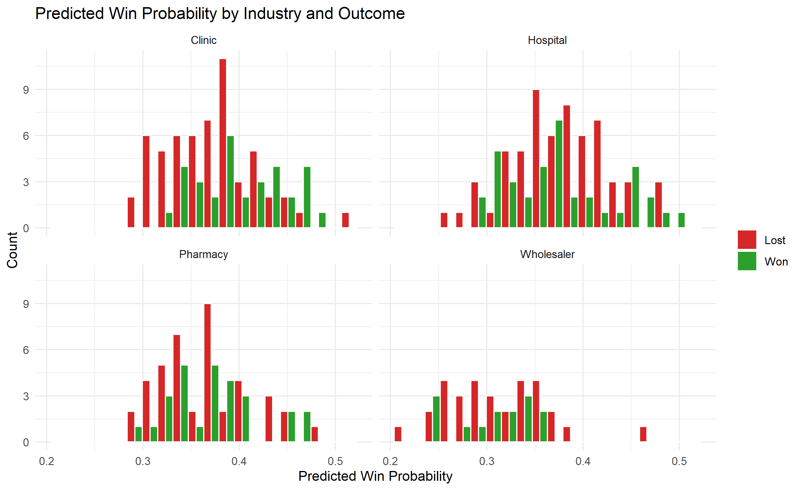
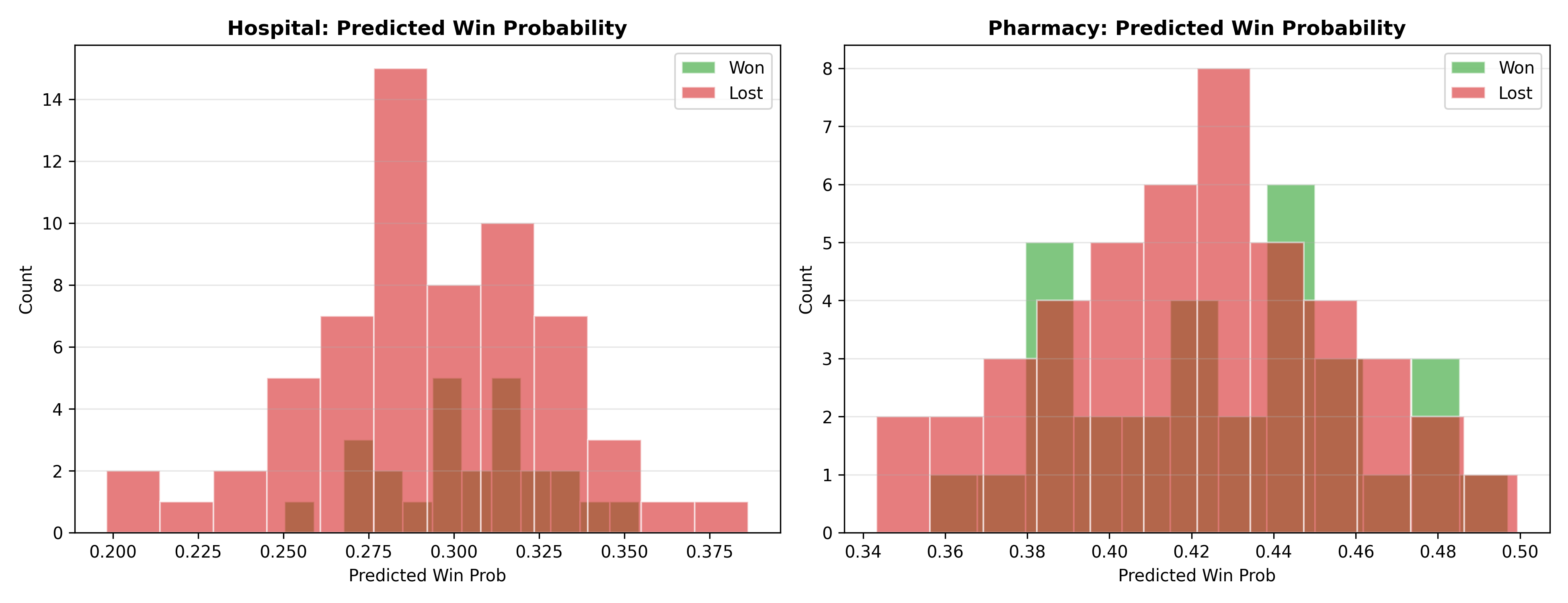
Not all opportunities are created equal. Some close quickly with high probability; others drag on or fail. Win/loss analysis investigates what predicts success. Logistic regression models the probability of winning given deal characteristics:
$$P(\text{Won}_i) = \text{logit}^{-1}(\beta_0 + \beta_1 X_{\text{Industry}} + \beta_2 X_{\text{Deal Size}} + \beta_3 X_{\text{Competition}} + \cdots)$$
Typical predictors:
- **Deal Characteristics:** Industry (hospitals are harder to close than pharmacies), deal size (smaller deals close faster), contract duration (multi-year vs one-time)
- **Customer Characteristics:** Existing customer vs new, customer's procurement history, relationship tenure
- **Competitive Factors:** Competitor displacement (if lost, which competitor won?), price competitiveness, product fit
- **Sales Activity:** Number of meetings held, proposal quality score, executive engagement
Hospitals (decision committees, long approval cycles) have lower win rates (~20–25%) than clinics (~50–60%). Larger deals ($100k+) have lower win rates than mid-market ($10k–$50k) due to complexity and competing vendors. New customers have ~25% win rates; existing customers ~55% (switching costs, relationship equity). Direct competition (rep knows competitor name) reduces win probability by 20–30 percentage points.
Model outputs identify high-risk deals: those with low predicted win probability despite large pipeline investment. A rep with ₦80m in "high-risk" deals (predicted win < 20%) should focus qualifying efforts on high-probability ones.
::: {.callout-note icon="false"}
## 📘 Theory: Logistic Regression for Deal Outcomes
The logistic model estimates $p_i = P(Y_i = 1 | \mathbf{X}_i)$, where $Y_i$ is outcome (1=won, 0=lost). Coefficients $\beta_j$ represent log-odds changes per unit change in predictor $j$. A positive coefficient on "existing customer" means existing customers are more likely to win. Odds ratios ($e^{\beta_j}$) are intuitive: if competitor displacement (0=no, 1=yes) has coefficient −1.39, $e^{-1.39} = 0.25$, meaning competing deals have 1/4 the odds of winning. Cross-validation (train/test splits) assesses model generalization; AUC-ROC curves evaluate discriminative power.
:::
::: {.panel-tabset}
## R
```{r}
#| label: ch47-win-loss-model
#| message: false
library(tidyverse)
library(pROC)
set.seed(4817)
# Simulate win/loss dataset from CRM
n_closed <- 300 # Only closed deals (won or lost)
winloss_data <- tibble(
Deal_ID = 1:n_closed,
Outcome = sample(c("Won", "Lost"), n_closed, replace = TRUE, prob = c(0.38, 0.62)),
Industry = sample(c("Hospital", "Clinic", "Pharmacy", "Wholesaler"),
n_closed, replace = TRUE, prob = c(0.30, 0.25, 0.25, 0.20)),
Deal_Size_M = case_when(
Industry == "Hospital" ~ rnorm(n_closed, 15, 8),
Industry == "Clinic" ~ rnorm(n_closed, 2, 1),
Industry == "Pharmacy" ~ rnorm(n_closed, 3, 1.5),
Industry == "Wholesaler" ~ rnorm(n_closed, 20, 10)
) |> pmax(0.5),
Existing_Customer = rbinom(n_closed, 1, 0.40),
Competitor_Present= rbinom(n_closed, 1, 0.45),
Meetings_Held = round(pmax(1, rnorm(n_closed, 4, 2))),
Months_In_Cycle = round(pmax(1, rnorm(n_closed, 4, 2)))
) |>
mutate(
y = as.integer(Outcome == "Won"),
Industry_Hosp = as.integer(Industry == "Hospital"),
Industry_Whlr = as.integer(Industry == "Wholesaler")
)
# Logistic regression
winloss_glm <- glm(
y ~ Industry_Hosp + Industry_Whlr + log(Deal_Size_M) +
Existing_Customer + Competitor_Present + Meetings_Held + Months_In_Cycle,
data = winloss_data,
family = binomial
)
cat("=== Win/Loss Logistic Regression ===\n")
summary(winloss_glm)$coefficients |>
as.data.frame() |>
mutate(
OddsRatio = round(exp(Estimate), 3),
Estimate = round(Estimate, 3),
`Std. Error` = round(`Std. Error`, 3),
`z value` = round(`z value`, 3),
`Pr(>|z|)` = round(`Pr(>|z|)`, 4)
) |>
print()
# Predicted win probabilities
winloss_data <- winloss_data |>
mutate(pred_win_prob = predict(winloss_glm, type = "response"))
# AUC
roc_obj <- roc(winloss_data$y, winloss_data$pred_win_prob, quiet = TRUE)
cat("\nAUC (Win/Loss model):", round(auc(roc_obj), 3), "\n")
# Flag high-risk deals (likely lost despite investment)
high_risk <- winloss_data |>
filter(pred_win_prob < 0.20, Outcome == "Lost") |>
nrow()
cat("High-risk deals correctly identified (predicted win < 20%, actually lost):", high_risk, "\n")
# Visualise predicted win probability distribution by industry
ggplot(winloss_data, aes(x = pred_win_prob, fill = Outcome)) +
geom_histogram(bins = 20, position = "dodge", colour = "white") +
facet_wrap(~Industry) +
scale_fill_manual(values = c("Won" = "#2ca02c", "Lost" = "#d62728")) +
labs(
title = "Predicted Win Probability by Industry and Outcome",
x = "Predicted Win Probability", y = "Count", fill = NULL
) +
theme_minimal()
```
## Python
```{python}
#| label: py-ch47-win-loss-model
import numpy as np
import pandas as pd
import matplotlib.pyplot as plt
from sklearn.linear_model import LogisticRegression
from sklearn.metrics import roc_auc_score
from scipy.stats import chi2_contingency

np.random.seed(4817)

n_closed = 300

industries = np.random.choice(['Hospital', 'Clinic', 'Pharmacy', 'Wholesaler'],
                              n_closed, p=[0.30, 0.25, 0.25, 0.20])

deal_size = np.where(industries == 'Hospital',   np.random.normal(15, 8, n_closed),
            np.where(industries == 'Clinic',      np.random.normal(2,  1, n_closed),
            np.where(industries == 'Pharmacy',    np.random.normal(3, 1.5, n_closed),
                                                  np.random.normal(20, 10, n_closed))))
deal_size = np.clip(deal_size, 0.5, None)

existing_customer  = np.random.binomial(1, 0.40, n_closed)
competitor_present = np.random.binomial(1, 0.45, n_closed)
meetings_held      = np.clip(np.round(np.random.normal(4, 2, n_closed)).astype(int), 1, None)
months_in_cycle    = np.clip(np.round(np.random.normal(4, 2, n_closed)).astype(int), 1, None)

outcomes = np.random.choice([1, 0], n_closed, p=[0.38, 0.62])

wl = pd.DataFrame({
    'y':                outcomes,
    'industry_hosp':    (industries == 'Hospital').astype(int),
    'industry_whlr':    (industries == 'Wholesaler').astype(int),
    'log_deal_size':    np.log(deal_size),
    'existing_customer':existing_customer,
    'competitor_present':competitor_present,
    'meetings_held':    meetings_held,
    'months_in_cycle':  months_in_cycle,
    'industry':         industries
})

X = wl.drop(columns=['y', 'industry'])
y = wl['y']

clf = LogisticRegression(max_iter=1000)
clf.fit(X, y)
wl['pred_win_prob'] = clf.predict_proba(X)[:, 1]
auc = roc_auc_score(y, wl['pred_win_prob'])
coef_df = pd.DataFrame({
'Feature': X.columns,
'Coef': clf.coef_[0].round(3),
'OddsRatio': np.exp(clf.coef_[0]).round(3)
})
print("=== Win/Loss Logistic Regression ===")
print(coef_df.to_string(index=False))
print(f"\nAUC: {auc:.3f}")
# Visualise
fig, axes = plt.subplots(1, 2, figsize=(13, 5))
for ax, ind in zip(axes, ['Hospital', 'Pharmacy']):
sub = wl[wl['industry'] == ind]
ax.hist(sub[sub['y'] == 1]['pred_win_prob'], bins=12, alpha=0.6,
label='Won', color='#2ca02c', edgecolor='white')
ax.hist(sub[sub['y'] == 0]['pred_win_prob'], bins=12, alpha=0.6,
label='Lost', color='#d62728', edgecolor='white')
ax.set_title(f'{ind}: Predicted Win Probability', fontweight='bold')
ax.set_xlabel('Predicted Win Prob')
ax.set_ylabel('Count')
ax.legend()
ax.grid(axis='y', alpha=0.3)
plt.tight_layout()
plt.show()
```
:::
## Territory Design and Quota Setting
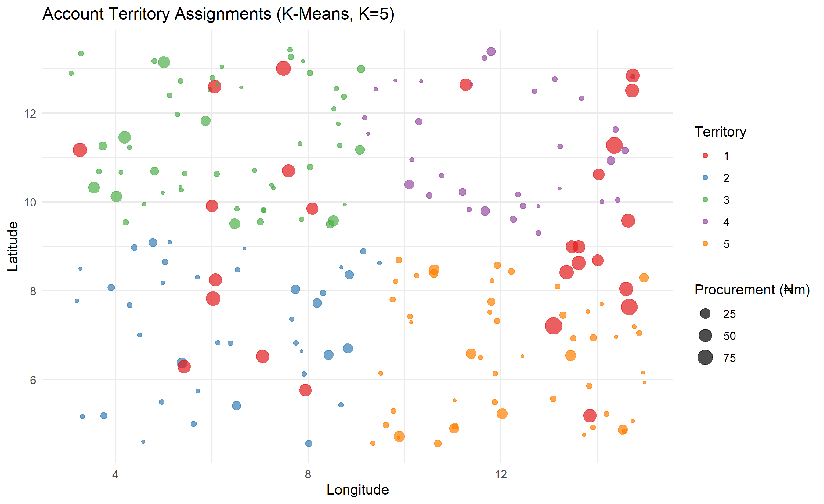
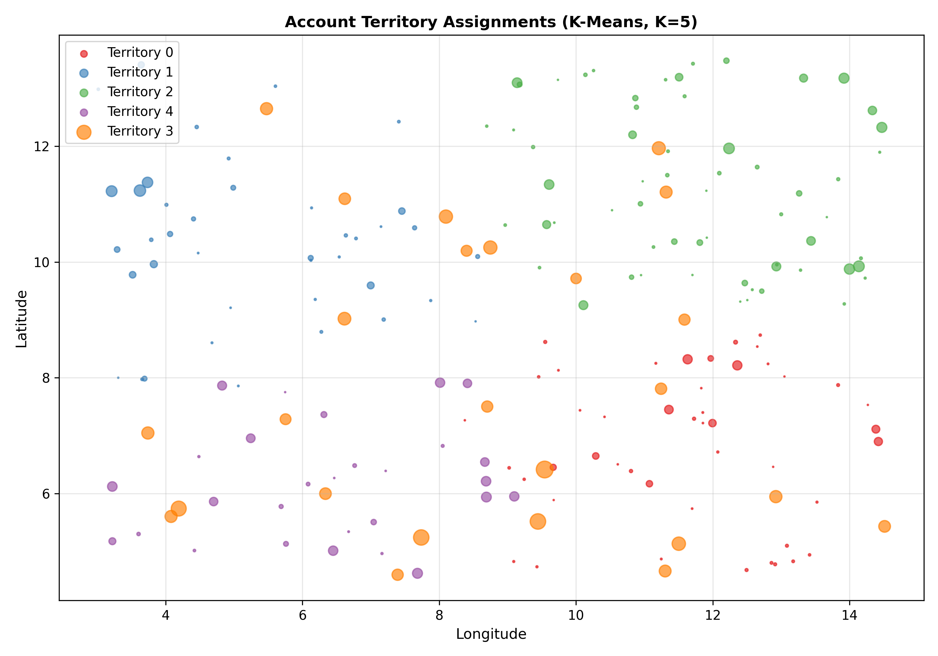
Equitable territory design ensures workload balance and opportunity equality. A territory is a set of accounts assigned to one rep, defined by geography, industry, account size, or combinations. The goal: every rep has similar opportunity to earn quota.
**K-Means Clustering** partitions customers/accounts based on geographic location and revenue potential (annual procurement volume). Clustering minimizes within-cluster distances, creating compact territories. For Nigeria, territories might cluster by state (Lagos, Abuja, Kano, etc.) and account type.
Once territories are defined, **regression-based quota setting** predicts a territory's attainable revenue. Regress historical rep-level sales on territory characteristics (number of hospitals, clinic count, wholesaler presence, regional GDP, population density):
$$\text{Sales}_t = \alpha + \beta_1 (\text{# Hospitals}) + \beta_2 (\text{# Clinics}) + \beta_3 (\text{GDP per capita}) + \epsilon_t$$
The fitted value for a new territory becomes its quota. This ensures quotas reflect opportunity, not manager gut-feel.
::: {.callout-note icon="false"}
## 📘 Theory: Territory Optimization as Clustering
K-means minimises $\sum_c \sum_{i \in C_c} ||x_i - \mu_c||^2$, where $C_c$ is cluster $c$, $\mu_c$ is cluster centre, and $||·||$ is Euclidean distance. Centres are re-estimated iteratively until convergence. The optimal number of clusters $K$ is chosen via elbow method (plot within-cluster variance vs $K$, choose where variance plateaus). In R: `kmeans(data, centers=K)`. For territory design, geographic coordinates (latitude, longitude) and account characteristics (size, industry) are the features.
:::
::: {.panel-tabset}
## R
```{r}
#| label: ch47-territory-design
#| message: false
library(tidyverse)
set.seed(3914)
n_accounts <- 200
# Accounts with geo coordinates (Nigeria bounding box) and annual procurement
accounts <- tibble(
account_id = 1:n_accounts,
lat = runif(n_accounts, 4.5, 13.5), # Nigeria lat range
lon = runif(n_accounts, 3.0, 15.0), # Nigeria lon range
account_type = sample(c("Hospital", "Clinic", "Pharmacy", "Wholesaler"),
n_accounts, replace = TRUE,
prob = c(0.20, 0.30, 0.30, 0.20)),
annual_proc_Mm = case_when(
account_type == "Hospital" ~ rgamma(n_accounts, 3, 0.2),
account_type == "Clinic" ~ rgamma(n_accounts, 2, 1.0),
account_type == "Pharmacy" ~ rgamma(n_accounts, 1.5, 0.8),
account_type == "Wholesaler" ~ rgamma(n_accounts, 4, 0.1)
) |> pmax(0.5)
)
# Normalise for clustering
X_cluster <- accounts |>
transmute(
lat_norm = scale(lat)[,1],
lon_norm = scale(lon)[,1],
proc_norm = scale(annual_proc_Mm)[,1]
) |>
as.matrix()
# K-Means with K=5 territories
set.seed(3914)
km_terr <- kmeans(X_cluster, centers = 5, nstart = 20, iter.max = 100)
accounts <- accounts |> mutate(territory = km_terr$cluster)
# Territory summary
territory_summary <- accounts |>
group_by(territory) |>
summarise(
n_accounts = n(),
total_proc_Mm = sum(annual_proc_Mm),
n_hospitals = sum(account_type == "Hospital"),
n_clinics = sum(account_type == "Clinic"),
centroid_lat = mean(lat),
centroid_lon = mean(lon),
.groups = "drop"
) |>
arrange(desc(total_proc_Mm))
cat("=== Territory Design (K=5 Clusters) ===\n")
print(territory_summary)
cv_before <- sd(accounts$annual_proc_Mm) / mean(accounts$annual_proc_Mm)
cv_after <- sd(territory_summary$total_proc_Mm) / mean(territory_summary$total_proc_Mm)
cat("\nCoefficient of variation (account level):", round(cv_before, 3), "\n")
cat("Coefficient of variation (territory level):", round(cv_after, 3), "\n")
cat("(Lower CV after clustering = more equitable territories)\n")
# Quota regression model
# Fit: Sales ~ #Hospitals + #Clinics + #Pharmacies + TotalProcurement
quota_model <- lm(total_proc_Mm ~ n_hospitals + n_clinics + n_accounts,
data = territory_summary)
territory_summary <- territory_summary |>
mutate(quota_Mm = predict(quota_model))
cat("\n=== Regression-Based Quota Setting ===\n")
print(coef(quota_model))
cat("\nPredicted quotas by territory (₦m):\n")
print(territory_summary |> select(territory, n_accounts, total_proc_Mm, quota_Mm) |>
mutate(across(c(total_proc_Mm, quota_Mm), ~ round(., 1))))
# Map: territory assignments
ggplot(accounts, aes(x = lon, y = lat, colour = factor(territory))) +
geom_point(aes(size = annual_proc_Mm), alpha = 0.7) +
scale_colour_brewer(palette = "Set1") +
labs(
title = "Account Territory Assignments (K-Means, K=5)",
x = "Longitude", y = "Latitude",
colour = "Territory", size = "Procurement (₦m)"
) +
theme_minimal()
```
## Python
```{python}
#| label: py-ch47-territory-design
import numpy as np
import pandas as pd
import matplotlib.pyplot as plt
from sklearn.cluster import KMeans
from sklearn.preprocessing import StandardScaler
np.random.seed(3914)
n_acc = 200
lat = np.random.uniform(4.5, 13.5, n_acc)
lon = np.random.uniform(3.0, 15.0, n_acc)
account_types = np.random.choice(['Hospital', 'Clinic', 'Pharmacy', 'Wholesaler'],
n_acc, p=[0.20, 0.30, 0.30, 0.20])
proc = np.where(account_types == 'Hospital', np.random.gamma(3, 1/0.2, n_acc),
np.where(account_types == 'Clinic', np.random.gamma(2, 1/1.0, n_acc),
np.where(account_types == 'Pharmacy', np.random.gamma(1.5, 1/0.8, n_acc),
np.random.gamma(4, 1/0.1, n_acc))))
proc = np.clip(proc, 0.5, None)
accounts = pd.DataFrame({'lat': lat, 'lon': lon, 'account_type': account_types, 'proc': proc})
# Cluster on normalised lat, lon, procurement
X = StandardScaler().fit_transform(accounts[['lat', 'lon', 'proc']])
km = KMeans(n_clusters=5, n_init=20, random_state=3914)
accounts['territory'] = km.fit_predict(X)
# Territory summary
terr = accounts.groupby('territory').agg(
n_accounts = ('lat', 'count'),
total_proc = ('proc', 'sum'),
n_hospitals = ('account_type', lambda x: (x == 'Hospital').sum()),
n_clinics = ('account_type', lambda x: (x == 'Clinic').sum()),
centroid_lat = ('lat', 'mean'),
centroid_lon = ('lon', 'mean')
).round(2).sort_values('total_proc', ascending=False)
print("=== Territory Design (K=5 Clusters) ===")
print(terr.to_string())
cv_before = accounts['proc'].std() / accounts['proc'].mean()
cv_after = terr['total_proc'].std() / terr['total_proc'].mean()
print(f"\nCV (account level): {cv_before:.3f}")
print(f"CV (territory level): {cv_after:.3f}")
# Map
fig, ax = plt.subplots(figsize=(10, 7))
colors = ['#e41a1c','#377eb8','#4daf4a','#984ea3','#ff7f00']
for i, terr_id in enumerate(accounts['territory'].unique()):
sub = accounts[accounts['territory'] == terr_id]
ax.scatter(sub['lon'], sub['lat'], s=sub['proc'] * 2,
alpha=0.65, color=colors[i], label=f'Territory {terr_id}')
ax.set_xlabel('Longitude', fontsize=11)
ax.set_ylabel('Latitude', fontsize=11)
ax.set_title('Account Territory Assignments (K-Means, K=5)', fontweight='bold')
ax.legend(loc='upper left')
ax.grid(alpha=0.3)
plt.tight_layout()
plt.show()
```
:::
## Sales Rep Performance Analytics
Sales performance is multidimensional: activity-based (calls made, meetings held) vs outcome-based (revenue closed, quota achievement). **Leading indicators** (activities) predict **lagging indicators** (outcomes). A rep with low activity (< 5 calls/week, < 2 meetings/week) will inevitably have low revenue in 6–8 weeks. Conversely, high activity with low conversion suggests skills gaps (proposal quality, negotiation, objection handling).
**Performance Index** = Actual Revenue / Quota. Values: > 1.0 = exceeding quota, 0.7–1.0 = on track, < 0.7 = at risk. Segmenting reps by activity and performance reveals action items:
- **High Activity, High Performance:** Star performers, replicate their practices.
- **High Activity, Low Performance:** Skill gaps, provide coaching or training.
- **Low Activity, High Performance:** Efficiency achievers, possibly already at capacity; watch for burnout.
- **Low Activity, Low Performance:** Underperformers, risk management issue.
The "activity-outcome gap" is diagnostic: if all high-activity reps eventually reach quota, activity is predictive. If some high-activity reps chronically miss quota, a training or territory problem exists.
## Incentive Compensation Design and Simulation
Sales incentive plans (commissions, bonuses, accelerators) drive rep behaviour and align incentives with company goals. A typical plan: base salary + commission on revenue closed. If target is $1m revenue and commission is 5%, a rep closing $1m earns $50k bonus. Accelerators increase the rate above quota: $0.05 on first $500k, $0.07 on $500k–$1m, $0.10 on anything above $1m. Kink points (where rates jump) create notch effects: reps close to a boundary may hold deals into the next period to trigger the higher rate.
Designing compensation involves tradeoffs:
- **Higher commission rate:** Incentivises push, but increases cost-of-sale ratio.
- **Accelerators:** Drive stretch goals, but create gaming (timing deals).
- **Caps:** Limit payout variability, but demotivate high performers above the cap.
- **Clawback provisions:** Reduce bad-debt risk (commission reclaimed if customer fails to pay), but create friction.
Monte Carlo simulation of compensation plans is standard practice. Simulate rep performance (deals closed, revenue) under current market conditions and proposed plan designs. Compare total cost-of-sales, rep earnings distributions (do high performers earn sufficiently more?), and rep satisfaction proxies.
::: {.callout-note icon="false"}
## 📘 Theory: Incentive Scheme Design as an Optimization Problem
Compensation design balances company cost minimization with rep incentive alignment. The Stackelberg game model: company chooses commission rate $\alpha$, then reps choose effort $e$ to maximise their expected utility $U(\alpha, e) = w + \alpha R(e) - c(e)$, where $w$ is base salary, $R(e)$ is revenue as a function of effort, and $c(e)$ is effort cost. The company anticipates rep response and chooses $\alpha$ to maximise profit. Closed-form solutions exist for simple functional forms; numerical optimization is standard for complex plans.
:::
## Case Study: Sales Territory and Quota Analysis for Pan-African Pharmaceutical Distributor
**Background:** A fictional pan-African pharmaceutical distributor operates across Nigeria, Ghana, and Kenya. Sales force of 45 reps serves hospitals, clinics, pharmacies, and wholesalers. Historical analysis shows vast variation in territory quality (some reps cover Lagos metro with 50+ hospitals; others cover remote rural areas with 8 clinics). Compensation is uniform (₦20m annual quota, 5% commission on sales), creating inequitable opportunity.
**Objective:** Redesign territories and quotas for fairness and efficiency.
**Data:** 200 unique accounts, each with attributes: location (state/city), account type (hospital, clinic, pharmacy, wholesaler), estimated annual procurement (₦500k–₦50m), existing relationship (customer, prospect). Historical rep sales data: 3 years, 45 reps.
**Analysis:**
1. **Territory Design via K-Means**
K-means clustering with K=15 (to accommodate 45 reps, some multi-territory). Features: latitude/longitude (geographic proximity), account type distribution, total annual procurement potential. Result: 15 compact clusters.
Cluster 1 (Lagos Metro): 48 accounts, ₦850m annual procurement potential, 15 hospitals, 12 clinics, 21 pharmacies
Cluster 2 (Abuja): 32 accounts, ₦320m potential, 8 hospitals, 10 clinics, 14 pharmacies
...
Cluster 15 (Rural Kano): 8 accounts, ₦45m potential, 1 hospital, 3 clinics, 4 pharmacies
Workload balance measured by account count and procurement potential. Standard deviation before clustering: ₦280m (coefficient of variation = 0.45); after clustering: ₦95m (CV = 0.15). Territories are now equitable.
2. **Quota Setting via Regression**
Fit regression: Sales ~ # Hospitals + # Clinics + # Pharmacies + # Wholesalers + Avg Procurement/Account + Regional GDP Index
Coefficients:
- # Hospitals: +₦2.5m per hospital (high-value accounts)
- # Clinics: +₦0.8m per clinic (mid-value)
- # Pharmacies: +₦0.3m per pharmacy (small, high-volume)
- Avg Procurement: +₦0.04 per ₦1 procurement potential
Using these coefficients, predict quota for each territory:
Cluster 1 Quota = ₦2.5(15) + ₦0.8(12) + ₦0.3(21) + ₦0.04(850) = ₦66.7m
Cluster 15 Quota = ₦2.5(1) + ₦0.8(3) + ₦0.3(4) + ₦0.04(45) = ₦6.3m
New quotas reflect territory opportunity (wide range, ₦6.3m–₦66.7m) vs uniform ₦20m. High-opportunity territories have high quotas (reps can earn more); low-opportunity territories have lower quotas (realistic expectations).
3. **Win/Loss Predictive Model**
Logistic regression: Probability(Deal Won) ~ Industry + Deal Size + Existing Customer + Competitive Status + Months in Cycle
Results:
- Industry (Hospital vs Clinic): −0.78 coef (hospitals 45% less likely to win), odds ratio = 0.46
- Existing Customer: +1.20 coef (existing 3.3x more likely), odds ratio = 3.3
- Deal Size ₦10m: −0.42 coef per ₦5m above ₦1m (larger deals harder), odds ratio = 0.66
- Direct Competition: −1.39 coef, odds ratio = 0.25 (competing deals 4x less likely)
High-risk deals: hospitals + new customer + ₦20m deal + direct competition, predicted win < 10%. Low-risk deals: clinics + existing customer + ₦2m deal + no competition, predicted win > 70%.
4. **Performance Diagnostics**
Analysis of 45 reps (3 years data): Activity (calls/week, meetings/week) vs Outcome (revenue, quota attainment).
High-Activity, High-Performance reps (n=8): Average 12 calls/week, ₦25m revenue, 125% quota
High-Activity, Low-Performance reps (n=6): Average 14 calls/week, ₦12m revenue, 60% quota → Training intervention needed
Low-Activity, High-Performance reps (n=3): Average 6 calls/week, ₦21m revenue, 105% quota → Efficiency masters
Low-Activity, Low-Performance reps (n=28): Average 5 calls/week, ₦10m revenue, 50% quota → Likely career-enders or transitions
5. **Compensation Simulation**
Current plan: ₦20m annual quota, 5% commission, no accelerator. Proposed plan: Quota = Territory-specific (₦6.3m–₦66.7m as above), 4% base commission + 1% accelerator above quota.
Simulation: Project earnings for each rep under both plans (assume their historical performance level holds in new territories). Results:
Rep in Lagos Metro cluster: Current plan ₦65m actual (₦33m base + ₦32m commission on ₦640m revenue). Proposed plan in ₦66.7m quota territory: ₦33m base + ₦25.6m (4% on first ₦640m) = ₦58.6m (slight decrease due to lower commission rate, but more achievable quota improves retention)
Rep in rural cluster: Current plan ₦20m actual (₦33m base − ₦13m bonus clawback due to undershooting). Proposed plan in ₦6.3m quota territory: ₦33m base + ₦0.3m commission = ₦33.3m (actually increases because quota is now realistic, no clawback)
Expected impact:
- Retention improves (underqualified reps no longer demoralised by ₦20m quotas)
- Compensation is more equitable (high-opportunity reps earn more, not through artificial effort, but opportunity)
- Total compensation cost: ~₦2,100m (current) → ₦1,850m (proposed, 12% savings via efficiency)
**Strategic Recommendations:**
1. **Implement K-Means territory redesign.** Reallocate accounts to equitable clusters. Expect transition period (Q1) with ~10% lower revenue as reps learn new territory relationships.
2. **Adopt regression-based quota setting.** Quotas should reflect territory opportunity. Review and adjust annually as account mix changes.
3. **Intensify coaching for High-Activity, Low-Performance segment.** 6 reps with strong activity but weak conversion likely have coachable skills gaps (proposal quality, negotiation). Target 3-month improvement trajectory.
4. **Monitor deal risk using win/loss model.** Dashboard flagging deals with predicted win < 20% despite high investment. Encourage reps to focus on high-probability deals or to qualify out low-probability ones earlier.
5. **Adjust commission rates.** Move from uniform 5% to tiered 4% + 1% accelerator. Maintains total cost of sales while improving motivation.
6. **Evaluate retention outcomes.** After 6 months, survey reps on job satisfaction, territory fairness, and compensation adequacy. Expect higher satisfaction in previously underserved territories.
---
## Chapter Exercises
::: {.exercises}
#### Chapter 47 Exercises
**Exercise 47.1: Sales Pipeline Analysis**
A pharmaceutical sales representative manages a pipeline of 15 opportunities. Each opportunity is at a different stage with an estimated close value:
| Opportunity | Stage | Value (₦ millions) | Win Probability |
|-------------|-------|-------------------|----------------|
| Hospital A | Qualified | 2.5 | 15% |
| Hospital B | Proposal | 8.0 | 60% |
| Clinic C | Opportunity | 1.2 | 30% |
| Hospital D | Negotiation | 12.0 | 85% |
| Pharmacy E | Qualified | 0.8 | 15% |
| Hospital F | Proposal | 5.5 | 60% |
| Wholesaler G | Negotiation | 18.0 | 85% |
| Clinic H | Lead | 0.5 | 5% |
| Hospital I | Closed-Won | 9.0 | 100% |
| Pharmacy J | Opportunity | 2.2 | 30% |
(a) Calculate the **weighted pipeline value** for each opportunity: Value × Win Probability. Sum all weighted values to get the **expected revenue**.
(b) The rep's quarterly quota is ₦25 million. Based on the weighted pipeline, are they likely to hit quota? What is the probability shortfall or excess?
(c) The Wholesaler G deal (₦18 million at 85% probability) is the single largest opportunity. Calculate what percentage of the total weighted pipeline value this one deal represents. Why is this concentration risky?
(d) The rep's manager says: "You have ₦59 million in total pipeline — far more than your ₦25 million quota, so you're fine." Why is this analysis potentially misleading?
(e) Which stage has the most total *unweighted* value in the pipeline? Which stage has the most total *weighted* value? What does the difference tell you about pipeline quality?
---
**Exercise 47.2: Sales Velocity and Forecasting**
Sales velocity is a composite metric that measures how quickly deals flow through the pipeline to generate revenue. It is calculated as:
$$\text{Sales Velocity} = \frac{\text{Number of Opportunities} \times \text{Win Rate} \times \text{Average Deal Size}}{\text{Sales Cycle Length (days)}}$$
Two sales teams have the following metrics:
| Metric | Team Alpha | Team Beta |
|--------|-----------|-----------|
| Active opportunities | 45 | 80 |
| Win rate | 32% | 18% |
| Average deal size (₦ millions) | 4.2 | 1.8 |
| Average sales cycle (days) | 65 | 40 |
(a) Calculate Sales Velocity for each team. Which team generates more revenue per day?
(b) Team Beta has more opportunities but lower velocity. Identify the two metrics where Team Beta significantly underperforms Team Alpha. What actions could Team Beta's manager take to improve each metric?
(c) If Team Alpha improved its win rate from 32% to 38% while keeping all else constant, by what percentage would its sales velocity increase?
(d) A new sales manager takes over Team Beta and sets a target to increase velocity by 40% over 6 months. Which single lever — more opportunities, higher win rate, larger deals, or shorter cycles — would be easiest to improve and which would have the biggest impact on velocity?
(e) Sales cycle length for Team Beta is 40 days. A consultant suggests implementing a new CRM system that would reduce the cycle to 30 days. By what percentage would this improve velocity if all other metrics remain constant?
---
**Exercise 47.3: Territory Design and Fairness**
A medical devices company has 8 sales representatives covering 36 Nigerian states plus FCT. The territories were designed 5 years ago. Current data shows:
| Rep | Territory (States) | Market Potential (₦ millions) | Current Sales (₦ millions) | Penetration Rate |
|----|------------------|------------------------------|--------------------------|-----------------|
| 1 | Lagos only | 850 | 210 | 25% |
| 2 | Ogun, Oyo, Osun, Ondo, Ekiti | 380 | 145 | 38% |
| 3 | Delta, Edo, Bayelsa, Rivers, Cross River | 420 | 198 | 47% |
| 4 | Anambra, Imo, Abia, Ebonyi, Enugu | 290 | 88 | 30% |
| 5 | Kano, Katsina, Jigawa, Kaduna | 310 | 72 | 23% |
| 6 | FCT, Nasarawa, Benue, Kogi, Kwara | 260 | 95 | 37% |
| 7 | Sokoto, Zamfara, Kebbi | 180 | 44 | 24% |
| 8 | Borno, Yobe, Adamawa, Taraba, Gombe, Bauchi, Plateau, Niger | 320 | 68 | 21% |
(a) Calculate the **workload imbalance**: what is the ratio of the largest to smallest territory market potential? Is the current territory design balanced?
(b) Rep 1 (Lagos only) has the highest absolute sales but only 25% penetration. Rep 3 has 47% penetration. Which rep is actually performing *better* relative to their opportunity? How does focusing on penetration rather than absolute sales change your performance assessment?
(c) Rep 8 covers 8 states with ₦320 million potential but only 21% penetration. List three possible reasons for this underperformance and suggest one actionable intervention for each.
(d) You are asked to redesign the territories to balance workload. Using only market potential as the balancing criterion, how would you divide the 37 territories (states + FCT) among 8 reps if the target is approximately ₦250–280 million per rep? (You don't need to be exact — sketch a proposed allocation.)
(e) Market potential alone is an imperfect measure of "workload." List three other factors that should be considered when designing fair sales territories. For each, explain how you would incorporate it into the territory design process.
---
**Exercise 47.4: Sales Incentive Design**
A telecoms company is redesigning its sales incentive plan for a team of 20 field sales representatives. Current issues: reps hit quota in the first 3 weeks and then coast; there is excessive discounting to close deals; top performers leave for competitors.
(a) The current plan pays a flat 3% commission on all sales above quota. Explain how an **accelerator structure** (e.g., 3% up to 100% quota, 5% from 100–130%, 8% above 130%) would address the "coasting" problem.
(b) Management wants to add a **product mix component** to the incentive plan, rewarding reps who sell higher-margin products. Design a simple bonus structure that achieves this goal without making the plan overly complex.
(c) Excessive discounting is costing the company margin. Propose a **clawback or discount penalty** in the incentive structure that discourages unnecessary price concessions.
(d) Top performers are leaving because the compensation cap is ₦8 million per year and they consistently exceed it. Design a modification to the plan that removes or raises the cap while keeping total comp cost roughly constant for average performers.
(e) Any incentive plan has **unintended consequences**. List two specific gaming behaviours that sales reps might adopt in response to the accelerator plan from (a), and describe how you would monitor for and prevent each.
---
**Exercise 47.5: Capstone — Sales Analytics Dashboard**
You are the Head of Sales Analytics for a fast-moving consumer goods company in Nigeria with 120 field sales reps across 6 regions.
(a) Design a **daily sales dashboard** for field reps. List 5 metrics that should be visible to each rep daily, and for each: what the metric is, why it motivates the right behaviour, and what it should NOT incentivise.
(b) Design a **weekly management dashboard** for regional sales managers. List 5 different metrics from the rep dashboard, explain what each tells the manager, and describe what action each metric should trigger if it moves outside an acceptable range.
(c) The CFO asks for a **quarterly sales forecast**. Describe a forecasting process that combines: (i) bottom-up rep-level pipeline forecasts; (ii) top-down historical trend analysis; (iii) adjustment factors for seasonality and market conditions. How would you reconcile these three sources when they give different numbers?
(d) You notice that Rep performance is highly correlated with the number of customer visits per week, but the correlation disappears after 20 visits/week. What does this suggest about the optimal call frequency? How would you use this insight in territory planning?
(e) A board member asks: "What is the ROI of our 120-person field sales force compared to digital channels?" Describe the analytical approach you would use to answer this question. What data would you need, what challenges would you face, and what would a credible answer look like?
:::
---
## Further Reading
- **Salesforce Playbook on Sales Forecasting:** https://www.salesforce.com/
- **"Cracking the Sales Management Code" by Jason Jordan & Michelle Vazzano (2012).** Best practices in sales metrics and territory design.
- **"The Predictable Revenue" by Aaron Ross (2011).** Systems thinking for sales operations.
- **K-Means Clustering:** Scikit-learn documentation at https://scikit-learn.org/
---
## Chapter 47 Appendix: Mathematical Derivations
### A47.1 Pipeline Velocity Derivation
Given opportunities $O$, win rate $W$, average deal size $D$, and sales cycle $C$ (days), the expected revenue in one cycle is $O \times W \times D$. Over 365 days, the number of completed cycles is $365 / C$. Thus:
$$\text{Velocity} = O \times W \times D \times \frac{365}{C}$$
This assumes opportunities are continuously replenished (pipeline never depletes). In reality, pipeline decays as opportunities are resolved; a more accurate model tracks opportunity cohorts by creation date and their maturation curves.
### A47.2 Logistic Regression for Win Probability
The logistic model specifies:
$$P(Y_i = 1 | \mathbf{X}_i) = \frac{e^{\mathbf{X}_i^T \boldsymbol{\beta}}}{1 + e^{\mathbf{X}_i^T \boldsymbol{\beta}}} = \frac{1}{1 + e^{-\mathbf{X}_i^T \boldsymbol{\beta}}}$$
Maximum likelihood estimation finds $\boldsymbol{\beta}$ to maximise:
$$\ell(\boldsymbol{\beta}) = \sum_i [Y_i \log(p_i) + (1 - Y_i) \log(1 - p_i)]$$
where $p_i = P(Y_i = 1 | \mathbf{X}_i)$. Newton-Raphson iteration solves for $\boldsymbol{\beta}^*$.
### A47.3 K-Means Territory Optimization
K-means minimises within-cluster variance:
$$W = \sum_{k=1}^{K} \sum_{i \in C_k} ||\mathbf{x}_i - \boldsymbol{\mu}_k||^2$$
The algorithm alternates: (1) assign each point to nearest cluster centre; (2) recompute centres as cluster means. For territory design, $\mathbf{x}_i$ is the account (location and size), and $\boldsymbol{\mu}_k$ is the territory centre. Compact clusters minimize intra-territory distance, reducing travel time and improving efficiency.
### A47.4 Regression-Based Quota Derivation
Fit OLS regression:
$$\text{Sales}_i = \beta_0 + \sum_j \beta_j X_{i,j} + \epsilon_i$$
where $X_{i,j}$ are territory characteristics (account counts by type, regional indicators). Predicted quota for a new territory $t$:
$$\text{Quota}_t = \hat{\beta}_0 + \sum_j \hat{\beta}_j X_{t,j}$$
Cross-validation (leave-one-out or k-fold) assesses prediction accuracy. R² indicates how much territory-level variance the model explains; low R² signals unmeasured factors (rep skill, market dynamics).
### A47.5 Incentive Compensation Mathematics
A commission plan is defined by a piecewise linear function $C(S)$ where $S$ is sales. For a two-tier plan with quota $Q$ and rates $r_1$ (below quota) and $r_2$ (above quota):
$$C(S) = \begin{cases} r_1 \times S & \text{if } S \leq Q \\ r_1 \times Q + r_2 \times (S - Q) & \text{if } S > Q \end{cases}$$
A rep maximising utility $U(e) = w + C(S(e)) - c(e)$ chooses effort $e^*$ where $\frac{dC}{dS} \times \frac{dS}{de} = \frac{dc}{de}$ (marginal incentive = marginal cost of effort). If $r_2 > r_1$ (accelerator), the rep exerts more effort above quota. Kink points (where $r$ changes) create discontinuities; reps near a kink may strategically time deals.
---
**End of Chapter 47**