31 Cash Flow and Financial Forecasting

📋 Learning Objectives

Understand the distinction between cash flow and profit, and why cash forecasting is critical for business survival
Build a structured monthly cash flow model incorporating accounts receivable (DSO), accounts payable (DPO), and inventory (DIO)
Apply time series methods (ARIMA, Holt-Winters) to operating cash flows and adapt them for structural breaks
Estimate forecast intervals using quantile regression, a technique that predicts percentiles rather than means
Conduct sensitivity analysis using tornado diagrams to rank which assumptions drive greatest uncertainty
Use Monte Carlo simulation to quantify tail risk and generate a distribution of possible cash balances
Create a complete, production-ready cash flow forecasting dashboard for treasury decision-making

31.1 Why Cash Flow Is the Lifeblood of Business

The adage is true: “Revenue is vanity, profit is sanity, cash is reality.” A company can be profitable on the income statement yet face insolvency if its cash balance falls below zero. Cash flow differs from profit in two critical ways. Profit is accrual-based: revenue is recorded when earned (even if payment is 90 days away), and expenses are recorded when incurred (even if payment is 30 days later). Cash flow is timing-based: inflows occur when customers actually pay; outflows occur when suppliers and creditors demand payment.

Consider a Nigerian manufacturing firm that receives a ₦50 million contract in January but receives payment only in April (90-day terms). On the income statement, January revenue is ₦50 million. In cash flow, January inflow is zero. If the firm must pay suppliers ₦40 million in February (45-day terms from raw material purchase in January) and staff in January, the firm faces a March cash crisis even though January looks profitable.

Direct Cash Flow Method: Start with cash inflows (collections from customers) and deduct cash outflows (payments to suppliers, staff, lenders, tax authorities). The result is operating cash flow.

Indirect Method: Start with net income, add back non-cash charges (depreciation, amortisation), adjust for changes in working capital (accounts receivable increase = cash outflow; accounts payable increase = cash inflow), to arrive at operating cash flow.

In practice, the direct method is more intuitive for forecasting: you forecast collections and disbursements independently, then combine them. This chapter uses the direct method.

The 13-week rolling cash forecast is the treasury standard: a detailed week-by-week (or in our case, month-by-month) projection of cash inflows and outflows for the next quarter. Treasurers use this to identify shortfalls and arrange borrowing in advance, avoiding panic and expensive emergency credit lines.

31.2 Components of a Cash Flow Forecast

A complete monthly cash flow model has several interconnected components:

Operating Inflows: Collections from customers. If monthly revenue is ₦V_t, and the Days Sales Outstanding (DSO) is D days, collections in month \(t\) include: - 30-day DSO: 70% from month \(t\), 30% from month \(t-1\). - 60-day DSO: 50% from month \(t\), 30% from month \(t-1\), 20% from month \(t-2\).

For Nigerian businesses, DSO varies widely: ₦0–15 days for FMCG retail (cash on collection), ₦45–90 days for manufacturing (business-to-business).

Operating Outflows: Payments to suppliers and staff. If Cost of Goods Sold (COGS) is ₦C_t and operating expenses are ₦E_t: - Supplier payments depend on Days Payable Outstanding (DPO). A 45-day DPO means you pay in month \(t+1\) for goods received in month \(t\). - Salary is typically paid in the same month earned.

Inventory: The cash cycle involves inventory financing. If you buy ₦10 million of stock and hold it for 30 days (Days Inventory Outstanding, DIO) before selling, your working capital is tied up for that month plus the DSO.

Capital Expenditure (CapEx): One-time or planned purchases of equipment, vehicles, or property.

Debt Service: Scheduled loan repayments (principal + interest).

Taxes: Corporate income tax, VAT (if you’re a net payer), customs duties.

The structure is: \[\text{Cash Flow}_t = \text{Collections}_t - \text{Supplier Payments}_t - \text{Payroll}_t - \text{CapEx}_t - \text{Debt Service}_t - \text{Taxes}_t\] \[\text{Ending Cash}_t = \text{Beginning Cash}_t + \text{Cash Flow}_t\]

📘 Theory: Working Capital Cycle

The Cash Conversion Cycle (CCC) is the time it takes for cash invested in operations to return to the firm: \[\text{CCC} = \text{DIO} + \text{DSO} - \text{DPO}\] For example, DIO = 30 (days holding inventory), DSO = 45 (days to collect), DPO = 30 (days to pay suppliers): \[\text{CCC} = 30 + 45 - 30 = 45 \text{ days}\] A firm needs to finance 45 days of operations. Reducing CCC (e.g., by negotiating longer DPO with suppliers) frees up cash.

🔑 Key Formula

Cash Collections with DSO: \[\text{Collections}_t = V_t \times \frac{\text{DSO}_{\text{current}}}{30} + V_{t-1} \times \left(1 - \frac{\text{DSO}_{\text{current}}}{30}\right)\] For simplicity, if DSO = 30, all revenue collected in the current month. If DSO = 60, 50% current, 50% next month.

Show code

library(tidyverse)
library(lubridate)
library(knitr)

# Build a 24-month cash flow model for a synthetic Nigerian manufacturing firm
# Base case: steady growth with seasonal peaks

set.seed(111)
months_future <- 24
dates <- seq(from = as.Date("2023-01-01"), by = "month", length.out = months_future)

# Assumptions (all in ₦ millions)
dso_days <- 45          # Days sales outstanding
dpo_days <- 30          # Days payable outstanding
dio_days <- 25          # Days inventory outstanding

# Monthly revenue with trend and seasonality
base_revenue <- 50
trend_factor <- seq(1, 1.4, length.out = months_future)
monthly_seasonal <- c(0.9, 0.95, 1.0, 0.95, 0.95, 1.0,
                      1.2, 1.3, 1.0, 0.95, 1.1, 1.2)  # Q4 peak
seasonal_vector <- rep(monthly_seasonal, length.out = months_future)

revenue <- base_revenue * trend_factor * seasonal_vector +
           rnorm(months_future, 0, 2)
revenue <- pmax(revenue, 15)

# COGS and Operating Expenses as % of revenue
cogs_pct <- 0.55
opex_pct <- 0.25

cogs <- revenue * cogs_pct
opex <- revenue * opex_pct

# Build cash flow model
cf_model <- data.frame(
  month = 1:months_future,
  date = dates,
  revenue = revenue,
  cogs = cogs,
  opex = opex
) |>
  mutate(
    # Collections: with 45-day DSO, ~1.5 months delay
    lag_revenue = lag(revenue, 1),
    lag_revenue_2 = lag(revenue, 2),
    collections = revenue * (30 - dso_days) / 30 +
                  ifelse(is.na(lag_revenue), 0, lag_revenue * (dso_days - 0) / 30) +
                  ifelse(is.na(lag_revenue_2), 0, lag_revenue_2 * max(0, dso_days - 30) / 30),
    # Supplier payments: DPO = 30, so pay this month for goods from last month
    lag_cogs = lag(cogs, 1),
    supplier_payments = ifelse(is.na(lag_cogs), cogs * 0.5, lag_cogs),
    # Payroll and operating expenses paid in the same month
    payroll_and_opex = opex,
    # Fixed monthly capex
    capex = c(rep(5, 12), rep(8, 12)),  # ₦5-8M per month
    # Loan repayment (quarterly, ₦3M per quarter)
    loan_repayment = c(3, 0, 0, 3, 0, 0, 3, 0, 0, 3, 0, 0,
                       3, 0, 0, 3, 0, 0, 3, 0, 0, 3, 0, 0),
    # Tax (quarterly, ~20% of gross profit)
    tax_payment = pmax(0, (revenue - cogs) * 0.20 *
                   c(0, 0, 1, 0, 0, 0, 0, 0, 1, 0, 0, 0,
                     0, 0, 1, 0, 0, 0, 0, 0, 1, 0, 0, 0) / 30)
  ) |>
  mutate(
    operating_cf = collections - supplier_payments - payroll_and_opex,
    free_cf = operating_cf - capex - loan_repayment - tax_payment,
    beginning_cash = c(50, rep(NA_real_, months_future - 1)),  # Start with ₦50M
  )

# Fill in beginning cash values
for (i in 2:nrow(cf_model)) {
  cf_model$beginning_cash[i] <- cf_model$beginning_cash[i - 1] + cf_model$free_cf[i - 1]
}

cf_model <- cf_model |>
  mutate(
    ending_cash = beginning_cash + free_cf,
    min_cash_alert = ifelse(ending_cash < 10, "⚠️ LOW", "OK")
  )

# Display model
cat("24-Month Cash Flow Model for Nigerian Manufacturer\n")
#> 24-Month Cash Flow Model for Nigerian Manufacturer
cat("(₦ millions)\n\n")
#> (₦ millions)

summary_cf <- cf_model |>
  select(month, date, revenue, collections, supplier_payments,
         payroll_and_opex, operating_cf, capex, free_cf, ending_cash, min_cash_alert) |>
  mutate(
    date = format(date, "%b %Y"),
    across(where(is.numeric), round, 1)
  )

# Show first 6 and last 6 months
cat("First 6 months:\n")
#> First 6 months:
print(kable(head(summary_cf, 6), format = "simple"))
#> 
#> 
#>  month  date        revenue   collections   supplier_payments   payroll_and_opex   operating_cf   capex   free_cf   ending_cash  min_cash_alert 
#> ------  ---------  --------  ------------  ------------------  -----------------  -------------  ------  --------  ------------  ---------------
#>      1  Jan 2023       45.5         -22.7                12.5               11.4          -46.6       5     -54.6          -4.6  ⚠️ LOW          
#>      2  Feb 2023       47.7          44.4                25.0               11.9            7.4       5       2.4          -2.2  ⚠️ LOW          
#>      3  Mar 2023       51.1          68.7                26.2               12.8           29.7       5      24.5          22.4  OK             
#>      4  Apr 2023       45.4          77.8                28.1               11.3           38.4       5      30.4          52.7  OK             
#>      5  May 2023       50.5          68.4                25.0               12.6           30.8       5      25.8          78.5  OK             
#>      6  Jun 2023       54.6          71.1                27.8               13.7           29.7       5      24.7         103.2  OK

cat("\n\nMonths 19-24:\n")
#> 
#> 
#> Months 19-24:
print(kable(tail(summary_cf, 6), format = "simple"))
#> 
#> 
#>       month  date        revenue   collections   supplier_payments   payroll_and_opex   operating_cf   capex   free_cf   ending_cash  min_cash_alert 
#> ---  ------  ---------  --------  ------------  ------------------  -----------------  -------------  ------  --------  ------------  ---------------
#> 19       19  Jul 2024       76.4          88.2                35.2               19.1           33.8       8      22.8         535.2  OK             
#> 20       20  Aug 2024       87.2         103.0                42.0               21.8           39.2       8      31.2         566.4  OK             
#> 21       21  Sep 2024       68.1         135.0                48.0               17.0           70.0       8      61.8         628.1  OK             
#> 22       22  Oct 2024       65.5         113.0                37.5               16.4           59.2       8      48.2         676.3  OK             
#> 23       23  Nov 2024       76.4          94.2                36.0               19.1           39.0       8      31.0         707.3  OK             
#> 24       24  Dec 2024       83.7         105.6                42.0               20.9           42.6       8      34.6         741.9  OK

# Key metrics
cat("\n\nKey Metrics (24-month period):\n")
#> 
#> 
#> Key Metrics (24-month period):
metrics <- data.frame(
  Metric = c("Total Revenue", "Total Collections", "Total Free Cash Flow",
             "Minimum Ending Cash", "Months with Cash < ₦10M", "Average Operating CF"),
  Value = c(
    paste0("₦", round(sum(cf_model$revenue, na.rm = TRUE), 1), "M"),
    paste0("₦", round(sum(cf_model$collections, na.rm = TRUE), 1), "M"),
    paste0("₦", round(sum(cf_model$free_cf, na.rm = TRUE), 1), "M"),
    paste0("₦", round(min(cf_model$ending_cash), 1), "M"),
    sum(cf_model$min_cash_alert == "⚠️ LOW", na.rm = TRUE),
    paste0("₦", round(mean(cf_model$operating_cf, na.rm = TRUE), 1), "M")
  )
)
print(kable(metrics, format = "simple"))
#> 
#> 
#> Metric                    Value    
#> ------------------------  ---------
#> Total Revenue             ₦1492.4M 
#> Total Collections         ₦2033M   
#> Total Free Cash Flow      ₦691.9M  
#> Minimum Ending Cash       ₦-4.6M   
#> Months with Cash < ₦10M   2        
#> Average Operating CF      ₦36.4M

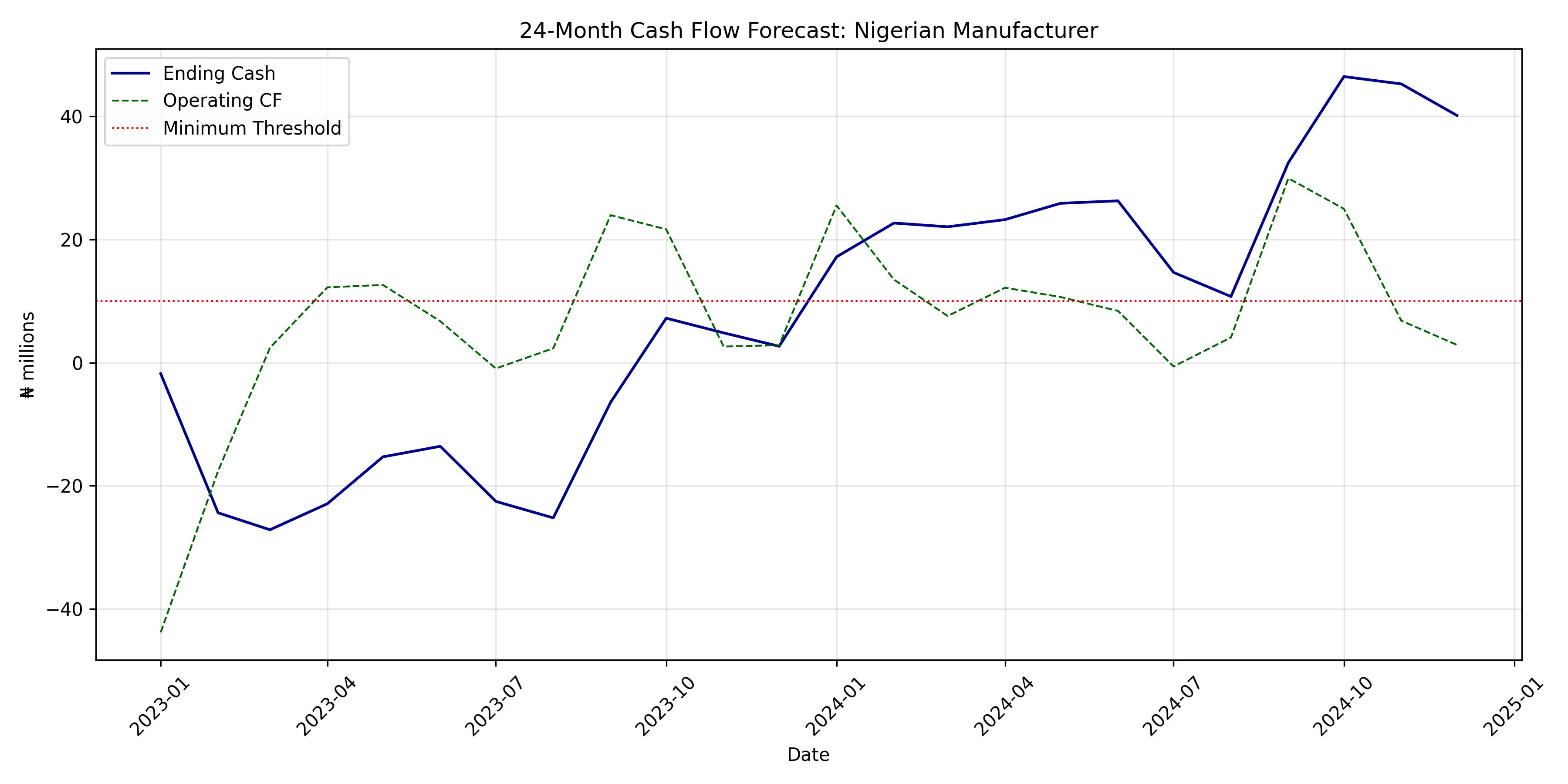
# Visualise cash balance and operating CF over time
cf_plot <- ggplot(cf_model, aes(x = date)) +
  geom_line(aes(y = ending_cash, colour = "Ending Cash"), linewidth = 1.2) +
  geom_line(aes(y = operating_cf, colour = "Operating CF"), linewidth = 0.8, linetype = "dashed") +
  geom_hline(yintercept = 10, linetype = "dotted", colour = "red", linewidth = 0.8) +
  scale_colour_manual(values = c("Ending Cash" = "darkblue", "Operating CF" = "darkgreen")) +
  labs(title = "24-Month Cash Flow Forecast: Nigerian Manufacturer",
       x = "Date", y = "₦ millions", colour = NULL) +
  theme_minimal() +
  theme(legend.position = "top", axis.text.x = element_text(angle = 45, hjust = 1))

print(cf_plot)

Show code

import pandas as pd
import numpy as np
from datetime import datetime, timedelta
import matplotlib.pyplot as plt

np.random.seed(111)
months_future = 24
dates = pd.date_range(start='2023-01-01', periods=months_future, freq='MS')

# Parameters
dso_days = 45
dpo_days = 30
dio_days = 25

# Revenue with trend and seasonality
base_revenue = 50
trend_factor = np.linspace(1, 1.4, months_future)
seasonal = np.tile([0.9, 0.95, 1.0, 0.95, 0.95, 1.0,
                    1.2, 1.3, 1.0, 0.95, 1.1, 1.2], 2)[:months_future]
revenue = base_revenue * trend_factor * seasonal + np.random.normal(0, 2, months_future)
revenue = np.maximum(revenue, 15)

cogs = revenue * 0.55
opex = revenue * 0.25

# Build cash flow model
cf_model = pd.DataFrame({
    'month': range(1, months_future + 1),
    'date': dates,
    'revenue': revenue,
    'cogs': cogs,
    'opex': opex
})

# Collections with 45-day DSO
cf_model['lag_revenue'] = cf_model['revenue'].shift(1)
cf_model['lag_revenue_2'] = cf_model['revenue'].shift(2)

cf_model['collections'] = (cf_model['revenue'] * (30 - dso_days) / 30 +
                           cf_model['lag_revenue'].fillna(0) * (min(dso_days, 30)) / 30 +
                           cf_model['lag_revenue_2'].fillna(0) * max(0, dso_days - 30) / 30)

# Supplier payments with 30-day DPO
cf_model['lag_cogs'] = cf_model['cogs'].shift(1)
cf_model['supplier_payments'] = cf_model['lag_cogs'].fillna(cf_model['cogs'] * 0.5)

# Other payments
cf_model['payroll_and_opex'] = cf_model['opex']
cf_model['capex'] = np.concatenate([np.full(12, 5), np.full(12, 8)])
cf_model['loan_repayment'] = np.tile([3, 0, 0], 8)[:months_future]

tax_pattern = np.tile([0, 0, 1, 0, 0, 0, 0, 0, 1, 0, 0, 0], 2)[:months_future]
cf_model['tax_payment'] = np.maximum(0, (cf_model['revenue'] - cf_model['cogs']) *
                                      0.20 * tax_pattern / 30)

# Calculate cash flows
cf_model['operating_cf'] = (cf_model['collections'] - cf_model['supplier_payments'] -
                            cf_model['payroll_and_opex'])
cf_model['free_cf'] = (cf_model['operating_cf'] - cf_model['capex'] -
                       cf_model['loan_repayment'] - cf_model['tax_payment'])

# Cumulative cash balance (compute both beginning and ending in lockstep)
cf_model['beginning_cash'] = 0.0
cf_model['ending_cash'] = 0.0
cf_model.loc[0, 'beginning_cash'] = 50
cf_model.loc[0, 'ending_cash'] = 50 + cf_model.loc[0, 'free_cf']
for i in range(1, len(cf_model)):
    cf_model.loc[i, 'beginning_cash'] = cf_model.loc[i-1, 'ending_cash']
    cf_model.loc[i, 'ending_cash'] = cf_model.loc[i, 'beginning_cash'] + cf_model.loc[i, 'free_cf']

print("24-Month Cash Flow Model for Nigerian Manufacturer")
#> 24-Month Cash Flow Model for Nigerian Manufacturer
print("(₦ millions)\n")
#> (₦ millions)

display_cols = ['month', 'date', 'revenue', 'collections', 'supplier_payments',
                'payroll_and_opex', 'operating_cf', 'capex', 'free_cf', 'ending_cash']
display_df = cf_model[display_cols].copy()
display_df['date'] = display_df['date'].dt.strftime('%b %Y')
for col in display_df.columns[2:]:
    display_df[col] = display_df[col].round(1)

print("First 6 months:")
#> First 6 months:
print(display_df.head(6).to_string(index=False))
#>  month     date  revenue  collections  supplier_payments  payroll_and_opex  operating_cf  capex  free_cf  ending_cash
#>      1 Jan 2023     42.7        -21.4               11.8              10.7         -43.8      5    -51.8         -1.8
#>      2 Feb 2023     49.1         18.2               23.5              12.3         -17.6      5    -22.6        -24.4
#>      3 Mar 2023     54.7         43.1               27.0              13.7           2.4      5     -2.8        -27.1
#>      4 Apr 2023     49.3         54.6               30.1              12.3          12.2      5      4.2        -22.9
#>      5 May 2023     49.2         52.0               27.1              12.3          12.6      5      7.6        -15.3
#>      6 Jun 2023     53.4         47.1               27.1              13.4           6.7      5      1.7        -13.6

print("\n\nMonths 19-24:")
#> 
#> 
#> Months 19-24:
print(display_df.tail(6).to_string(index=False))
#>  month     date  revenue  collections  supplier_payments  payroll_and_opex  operating_cf  capex  free_cf  ending_cash
#>     19 Jul 2024     81.3         55.8               36.1              20.3          -0.6      8    -11.6         14.6
#>     20 Aug 2024     87.1         70.6               44.7              21.8           4.1      8     -3.9         10.7
#>     21 Sep 2024     66.6         94.5               47.9              16.6          29.9      8     21.7         32.5
#>     22 Oct 2024     64.7         77.8               36.6              16.2          25.0      8     14.0         46.5
#>     23 Nov 2024     74.1         60.9               35.6              18.5           6.8      8     -1.2         45.3
#>     24 Dec 2024     83.8         64.6               40.8              20.9           2.9      8     -5.1         40.1

print("\n\nKey Metrics (24-month period):")
#> 
#> 
#> Key Metrics (24-month period):
metrics = {
    'Total Revenue': f"₦{cf_model['revenue'].sum():.1f}M",
    'Total Collections': f"₦{cf_model['collections'].sum():.1f}M",
    'Total Free CF': f"₦{cf_model['free_cf'].sum():.1f}M",
    'Minimum Ending Cash': f"₦{cf_model['ending_cash'].min():.1f}M",
    'Months Cash < ₦10M': sum(cf_model['ending_cash'] < 10),
    'Avg Operating CF': f"₦{cf_model['operating_cf'].mean():.1f}M"
}
for k, v in metrics.items():
    print(f"{k}: {v}")
#> Total Revenue: ₦1496.3M
#> Total Collections: ₦1333.6M
#> Total Free CF: ₦-9.9M
#> Minimum Ending Cash: ₦-27.1M
#> Months Cash < ₦10M: 12
#> Avg Operating CF: ₦7.1M

# Plot
fig, ax = plt.subplots(figsize=(12, 6))
ax.plot(cf_model['date'], cf_model['ending_cash'], label='Ending Cash',
        linewidth=1.5, color='darkblue')
ax.plot(cf_model['date'], cf_model['operating_cf'], label='Operating CF',
        linewidth=1, linestyle='--', color='darkgreen')
ax.axhline(y=10, color='red', linestyle=':', linewidth=1, label='Minimum Threshold')
ax.set_xlabel('Date')
ax.set_ylabel('₦ millions')
ax.set_title('24-Month Cash Flow Forecast: Nigerian Manufacturer')
ax.legend()
ax.grid(True, alpha=0.3)
plt.xticks(rotation=45)
#> (array([19358., 19448., 19539., 19631., 19723., 19814., 19905., 19997.,
#>        20089.]), [Text(19358.0, 0, '2023-01'), Text(19448.0, 0, '2023-04'), Text(19539.0, 0, '2023-07'), Text(19631.0, 0, '2023-10'), Text(19723.0, 0, '2024-01'), Text(19814.0, 0, '2024-04'), Text(19905.0, 0, '2024-07'), Text(19997.0, 0, '2024-10'), Text(20089.0, 0, '2025-01')])
plt.tight_layout()
plt.show()

📝 Section 26.2 Review Questions

Explain the difference between a 30-day DSO and a 60-day DSO in terms of cash collections. How much cash is tied up in each case?
In the model above, if DPO increases from 30 to 45 days, what happens to the cash balance? Why?
Calculate the cash conversion cycle (CCC) for a firm with DIO = 40, DSO = 60, DPO = 35. What does this number mean?
A business reports ₦100M profit but ending cash balance is ₦5M (down from ₦50M). Hypothesize three reasons why profit did not convert to cash.
How would you modify the cash flow model to include a seasonal loan facility (e.g., overdraft that expires at year-end)?

31.3 Time Series Methods for Cash Flow: ARIMA with Structural Breaks

Operating cash flow (inflows minus outflows) exhibits time series properties: trends, seasonality, and random shocks. ARIMA models work well for forecasting aggregate cash flows over moderate horizons (3–6 months), but struggle when the business environment changes (currency devaluation, policy shifts, supply disruptions).

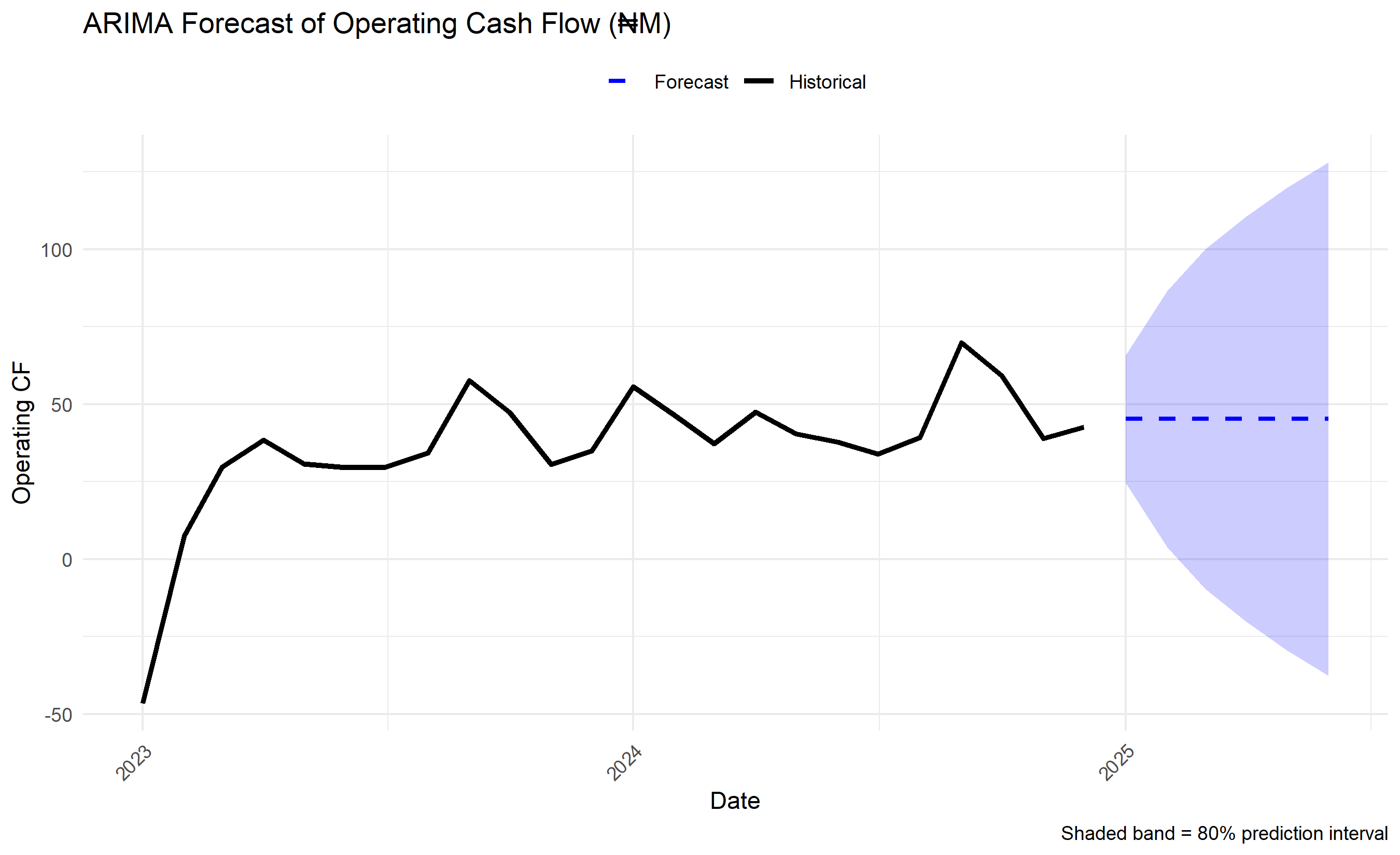
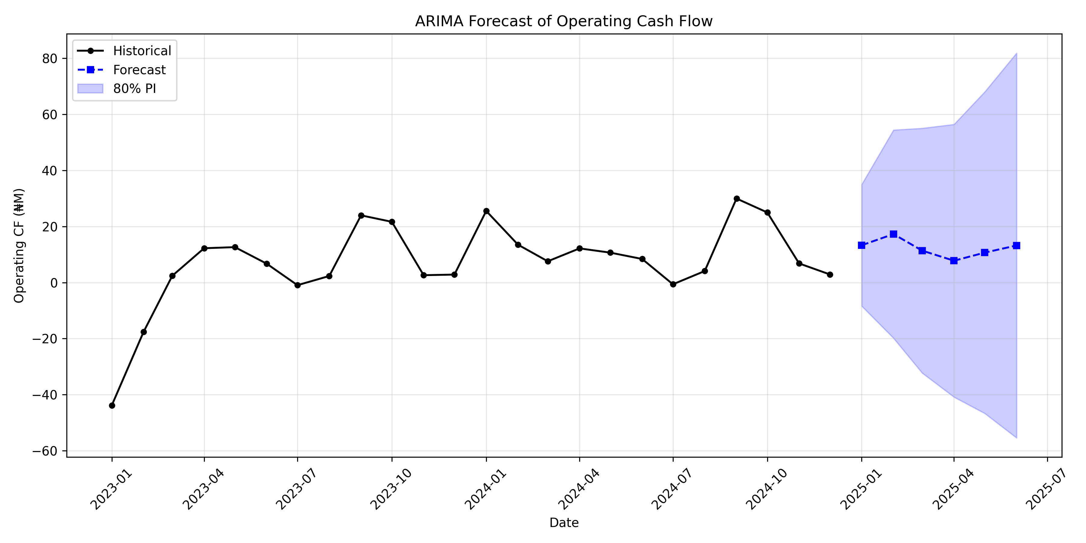
We fit ARIMA to the operating cash flows from the model above and forecast 6 months ahead. We then discuss limitations and the role of structural breaks.

📘 Theory: ARIMA for Cash Flow

An ARIMA(p, d, q) model on operating cash flow \(\text{CF}_t\) is: \[(1 - \phi_1 B - \cdots - \phi_p B^p)(1 - B)^d \text{CF}_t = (1 + \theta_1 B + \cdots + \theta_q B^q) \epsilon_t\] - \(d=1\) (first differencing) for a trending cash flow. - \(d=0\) if the series is stationary around a mean. - Seasonal ARIMA adds seasonal differencing and AR/MA terms at lags 12 (for monthly data).

When a structural break occurs (e.g., revenue drops 20% due to new regulation), the historical ARIMA coefficients become invalid. The model predicts the old mean, not the new state.

🔑 Key Formula

ARIMA(1,1,1) Specification: \[(1 - \phi_1 B)(1 - B) \text{CF}_t = (1 + \theta_1 B) \epsilon_t\] Expanding: \[\text{CF}_t = (1 + \phi_1) \text{CF}_{t-1} - \phi_1 \text{CF}_{t-2} + \epsilon_t + \theta_1 \epsilon_{t-1}\] This captures a random walk with drift (trend) plus moving average smoothing.

Show code

library(tidyverse)
library(forecast)
library(tseries)

# Use the cash flow model from above
# Extract operating CF (already computed in cf_model)
operating_cf_series <- cf_model$operating_cf[!is.na(cf_model$operating_cf)]
dates_cf <- cf_model$date[!is.na(cf_model$operating_cf)]

cat("Fitting ARIMA to Operating Cash Flow\n")
#> Fitting ARIMA to Operating Cash Flow
cat("Series: Months 1-24 of operating CF\n\n")
#> Series: Months 1-24 of operating CF

# Check stationarity
adf_test <- adf.test(operating_cf_series)
cat("Augmented Dickey-Fuller test:\n")
#> Augmented Dickey-Fuller test:
cat(sprintf("Test Statistic: %.4f\n", adf_test$statistic))
#> Test Statistic: -4.5825
cat(sprintf("P-value: %.4f\n", adf_test$p.value))
#> P-value: 0.0100
cat(sprintf("Interpretation: Series is %s\n\n",
            ifelse(adf_test$p.value < 0.05, "stationary", "non-stationary")))
#> Interpretation: Series is stationary

# Fit ARIMA using auto.arima
fit_arima <- auto.arima(operating_cf_series, trace = FALSE, stepwise = FALSE,
                        seasonal = FALSE)

cat("Best ARIMA Model:\n")
#> Best ARIMA Model:
print(fit_arima)
#> Series: operating_cf_series 
#> ARIMA(0,1,1) 
#> 
#> Coefficients:
#>          ma1
#>       0.7369
#> s.e.  0.2970
#> 
#> sigma^2 = 260:  log likelihood = -96.46
#> AIC=196.93   AICc=197.53   BIC=199.2

# Forecast 6 months ahead
fcst_arima <- forecast(fit_arima, h = 6)

# Create forecast dataframe
forecast_df <- data.frame(
  month = 25:30,
  date = seq(from = max(dates_cf) + months(1), by = "month", length.out = 6),
  forecast = fcst_arima$mean,
  lower_80 = fcst_arima$lower[, 1],
  upper_80 = fcst_arima$upper[, 1],
  lower_95 = fcst_arima$lower[, 2],
  upper_95 = fcst_arima$upper[, 2]
)

cat("\n6-Month Operating Cash Flow Forecast (₦M):\n\n")
#> 
#> 6-Month Operating Cash Flow Forecast (₦M):
print(forecast_df |>
        mutate(
          date = format(date, "%b %Y"),
          across(where(is.numeric) & !month, round, 1)
        ))
#>   month     date forecast lower_80 upper_80 lower_95 upper_95
#> 1    25 Jan 2025     45.3     24.6     65.9     13.6     76.9
#> 2    26 Feb 2025     45.3      3.8     86.7    -18.1    108.6
#> 3    27 Mar 2025     45.3     -9.6    100.1    -38.6    129.1
#> 4    28 Apr 2025     45.3    -20.3    110.8    -54.9    145.4
#> 5    29 May 2025     45.3    -29.4    120.0    -69.0    159.5
#> 6    30 Jun 2025     45.3    -37.6    128.1    -81.5    172.0

# Visualise: historical and forecast
all_dates <- c(dates_cf, forecast_df$date)
all_cf <- c(operating_cf_series, rep(NA, 6))
all_forecast <- c(rep(NA, length(operating_cf_series)), forecast_df$forecast)
all_lower <- c(rep(NA, length(operating_cf_series)), forecast_df$lower_80)
all_upper <- c(rep(NA, length(operating_cf_series)), forecast_df$upper_80)

viz_df <- data.frame(
  date = all_dates,
  actual = all_cf,
  forecast = all_forecast,
  lower = all_lower,
  upper = all_upper
)

ggplot(viz_df, aes(x = date)) +
  geom_line(aes(y = actual, colour = "Historical"), linewidth = 1.2) +
  geom_line(aes(y = forecast, colour = "Forecast"), linewidth = 1, linetype = "dashed") +
  geom_ribbon(aes(ymin = lower, ymax = upper), alpha = 0.2, fill = "blue") +
  scale_colour_manual(values = c("Historical" = "black", "Forecast" = "blue")) +
  labs(title = "ARIMA Forecast of Operating Cash Flow (₦M)",
       x = "Date", y = "Operating CF", colour = NULL,
       caption = "Shaded band = 80% prediction interval") +
  theme_minimal() +
  theme(legend.position = "top", axis.text.x = element_text(angle = 45, hjust = 1))

Show code


# Residual analysis
residuals_arima <- residuals(fit_arima)

cat("\n\nARIMA Residual Diagnostics:\n")
#> 
#> 
#> ARIMA Residual Diagnostics:
cat(sprintf("Mean residual: %.4f (should be ~0)\n", mean(residuals_arima)))
#> Mean residual: 2.0995 (should be ~0)
cat(sprintf("Std dev of residuals: %.4f\n", sd(residuals_arima)))
#> Std dev of residuals: 15.6236

# Ljung-Box test for autocorrelation
lb_test <- Box.test(residuals_arima, lag = 10, type = "Ljung-Box")
cat(sprintf("\nLjung-Box test for autocorrelation:\n"))
#> 
#> Ljung-Box test for autocorrelation:
cat(sprintf("Test Statistic: %.4f\n", lb_test$statistic))
#> Test Statistic: 5.9998
cat(sprintf("P-value: %.4f\n", lb_test$p.value))
#> P-value: 0.8153
cat(sprintf("Residuals are %s autocorrelated\n",
            ifelse(lb_test$p.value > 0.05, "NOT", "")))
#> Residuals are NOT autocorrelated

Show code

import pandas as pd
import numpy as np
from statsmodels.tsa.arima.model import ARIMA
from statsmodels.tsa.stattools import adfuller, kpss
import matplotlib.pyplot as plt

# Use the operating CF from the model
operating_cf = cf_model['operating_cf'].dropna().values

print("Fitting ARIMA to Operating Cash Flow")
#> Fitting ARIMA to Operating Cash Flow
print("Series: Months 1-24 of operating CF\n")
#> Series: Months 1-24 of operating CF

# Stationarity test
adf_result = adfuller(operating_cf)
print("Augmented Dickey-Fuller Test:")
#> Augmented Dickey-Fuller Test:
print(f"Test Statistic: {adf_result[0]:.4f}")
#> Test Statistic: -5.0470
print(f"P-value: {adf_result[1]:.4f}")
#> P-value: 0.0000
print(f"Series is {'stationary' if adf_result[1] < 0.05 else 'non-stationary'}\n")
#> Series is stationary

# Fit ARIMA
best_aic = np.inf
best_order = None

for p in range(0, 4):
    for d in range(0, 3):
        for q in range(0, 4):
            try:
                model = ARIMA(operating_cf, order=(p, d, q))
                fit = model.fit()
                if fit.aic < best_aic:
                    best_aic = fit.aic
                    best_order = (p, d, q)
            except:
                pass

print(f"Best ARIMA order: {best_order}")
#> Best ARIMA order: (2, 2, 1)
fit_arima = ARIMA(operating_cf, order=best_order).fit()
print(fit_arima.summary())
#>                                SARIMAX Results                                
#> ==============================================================================
#> Dep. Variable:                      y   No. Observations:                   24
#> Model:                 ARIMA(2, 2, 1)   Log Likelihood                 -85.259
#> Date:                Sun, 10 May 2026   AIC                            178.517
#> Time:                        15:43:31   BIC                            182.881
#> Sample:                             0   HQIC                           179.545
#>                                  - 24                                         
#> Covariance Type:                  opg                                         
#> ==============================================================================
#>                  coef    std err          z      P>|z|      [0.025      0.975]
#> ------------------------------------------------------------------------------
#> ar.L1          0.1657      0.162      1.023      0.307      -0.152       0.483
#> ar.L2         -0.6166      0.241     -2.562      0.010      -1.088      -0.145
#> ma.L1         -0.7771      0.236     -3.296      0.001      -1.239      -0.315
#> sigma2       122.3923     49.376      2.479      0.013      25.617     219.168
#> ===================================================================================
#> Ljung-Box (L1) (Q):                   0.05   Jarque-Bera (JB):                 1.10
#> Prob(Q):                              0.83   Prob(JB):                         0.58
#> Heteroskedasticity (H):               0.63   Skew:                             0.54
#> Prob(H) (two-sided):                  0.55   Kurtosis:                         2.77
#> ===================================================================================
#> 
#> Warnings:
#> [1] Covariance matrix calculated using the outer product of gradients (complex-step).

# Forecast
fcst = fit_arima.get_forecast(steps=6)
fcst_df = fcst.summary_frame()

forecast_df = pd.DataFrame({
    'month': range(25, 31),
    'date': pd.date_range(start=cf_model['date'].iloc[-1] + pd.DateOffset(months=1),
                          periods=6, freq='MS'),
    'forecast': fcst_df['mean'].values,
    'lower_80': fcst_df['mean_ci_lower'].values,
    'upper_80': fcst_df['mean_ci_upper'].values
})

print("\n\n6-Month Operating Cash Flow Forecast (₦M):\n")
#> 
#> 
#> 6-Month Operating Cash Flow Forecast (₦M):
print(forecast_df[['month', 'date', 'forecast', 'lower_80', 'upper_80']].round(1))
#>    month       date  forecast  lower_80  upper_80
#> 0     25 2025-01-01      13.3      -8.4      35.0
#> 1     26 2025-02-01      17.3     -19.8      54.4
#> 2     27 2025-03-01      11.4     -32.3      55.0
#> 3     28 2025-04-01       7.8     -40.8      56.4
#> 4     29 2025-05-01      10.7     -46.7      68.0
#> 5     30 2025-06-01      13.2     -55.4      81.8

# Plot
fig, ax = plt.subplots(figsize=(12, 6))
ax.plot(cf_model['date'], operating_cf, 'o-', label='Historical',
        linewidth=1.5, color='black', markersize=4)
ax.plot(forecast_df['date'], forecast_df['forecast'], 's--', label='Forecast',
        linewidth=1.5, color='blue', markersize=5)
ax.fill_between(forecast_df['date'], forecast_df['lower_80'], forecast_df['upper_80'],
                alpha=0.2, color='blue', label='80% PI')
ax.set_xlabel('Date')
ax.set_ylabel('Operating CF (₦M)')
ax.set_title('ARIMA Forecast of Operating Cash Flow')
ax.legend()
ax.grid(True, alpha=0.3)
plt.xticks(rotation=45)
#> (array([19358., 19448., 19539., 19631., 19723., 19814., 19905., 19997.,
#>        20089., 20179., 20270.]), [Text(19358.0, 0, '2023-01'), Text(19448.0, 0, '2023-04'), Text(19539.0, 0, '2023-07'), Text(19631.0, 0, '2023-10'), Text(19723.0, 0, '2024-01'), Text(19814.0, 0, '2024-04'), Text(19905.0, 0, '2024-07'), Text(19997.0, 0, '2024-10'), Text(20089.0, 0, '2025-01'), Text(20179.0, 0, '2025-04'), Text(20270.0, 0, '2025-07')])
plt.tight_layout()
plt.show()

Show code


# Residual diagnostics
residuals = fit_arima.resid
print(f"\n\nARIMA Residual Diagnostics:")
#> 
#> 
#> ARIMA Residual Diagnostics:
print(f"Mean residual: {residuals.mean():.4f} (should be ~0)")
#> Mean residual: -4.2516 (should be ~0)
print(f"Std dev: {residuals.std():.4f}")
#> Std dev: 16.7463

📝 Section 26.3 Review Questions

When would ARIMA be more appropriate than a structural cash flow model? When less?
What is a structural break, and how would you detect it in a cash flow series?
If a company’s currency devalues 30% mid-forecast, how would you adjust the ARIMA forecast?
Explain the trade-off between model complexity (ARIMA with seasonality) and interpretability (direct cash flow model).
How would you use walk-forward validation to backtest an ARIMA cash flow forecast?

31.4 Quantile Regression for Forecast Intervals

A point forecast (the mean) is insufficient for treasury decisions. A CFO needs to know: “With 90% confidence, what is the minimum cash balance?” This requires a forecast of the 10th percentile, not the mean. Quantile regression estimates the conditional quantile (e.g., the 10th, 50th, 90th percentile) of the target given features.

Quantile Regression Setup: Instead of minimising squared error (which estimates the mean), minimise the pinball loss: \[L_\tau(y, \hat{y}) = \begin{cases} \tau |y - \hat{y}| & \text{if } y \geq \hat{y} \\ (1 - \tau) |y - \hat{y}| & \text{if } y < \hat{y} \end{cases}\]

For \(\tau = 0.5\) (median), the pinball loss is symmetric (L1 loss). For \(\tau = 0.9\) (90th percentile), over-predictions are penalised less than under-predictions, pulling the fit toward higher values.

📘 Theory: Quantile Regression Loss

The pinball loss (also called asymmetric absolute loss or tilted L1 loss) is: \[L_\tau(y, \hat{y}) = (\tau - \mathbb{1}_{y < \hat{y}}) (y - \hat{y})\] Minimising this across a dataset fits a hyperplane (linear regression) or more complex model (nonlinear quantile regression) that estimates the conditional \(\tau\)-quantile. For \(\tau = 0.1\), the regression line is pulled toward the lower tail of the residuals; for \(\tau = 0.9\), toward the upper tail.

🔑 Key Formula

Pinball Loss for Quantile \(\tau\): \[\text{Loss}_\tau = \sum_{i=1}^{n} \begin{cases} \tau (y_i - \hat{y}_i) & \text{if } y_i > \hat{y}_i \\ (\tau - 1)(y_i - \hat{y}_i) & \text{if } y_i \leq \hat{y}_i \end{cases}\] This is equivalent to a weighted L1 loss, where over-predictions have weight \((1-\tau)\) and under-predictions have weight \(\tau\).

Show code

library(tidyverse)
library(quantreg)
library(lubridate)

# Build a dataset: lags of cash flow + calendar features as predictors
cf_data <- cf_model |>
  filter(!is.na(operating_cf)) |>
  mutate(
    lag_cf = lag(operating_cf, 1),
    lag_cf_3 = lag(operating_cf, 3),
    lag_cf_12 = lag(operating_cf, 12),
    trend = 1:n(),
    month_sin = sin(2 * pi * month(date) / 12),
    month_cos = cos(2 * pi * month(date) / 12),
    revenue_scaled = scale(revenue)[, 1]
  ) |>
  drop_na()

# Fit quantile regressions at three quantiles
tau_values <- c(0.1, 0.5, 0.9)  # 10th, 50th, 90th percentiles
qreg_models <- list()

for (tau in tau_values) {
  qr <- rq(operating_cf ~ lag_cf + lag_cf_3 + lag_cf_12 + trend +
             month_sin + month_cos + revenue_scaled,
           data = cf_data, tau = tau)
  qreg_models[[as.character(tau)]] <- qr

  cat(sprintf("\nQuantile Regression tau=%.2f (%.0f-th percentile):\n", tau, tau*100))
  print(summary(qr))
}
#> 
#> Quantile Regression tau=0.10 (10-th percentile):
#> 
#> Call: rq(formula = operating_cf ~ lag_cf + lag_cf_3 + lag_cf_12 + trend + 
#>     month_sin + month_cos + revenue_scaled, tau = tau, data = cf_data)
#> 
#> tau: [1] 0.1
#> 
#> Coefficients:
#>                coefficients   lower bd       upper bd      
#> (Intercept)      1.092914e+02 -1.797693e+308  1.797693e+308
#> lag_cf          -3.916600e-01 -1.797693e+308  1.797693e+308
#> lag_cf_3         1.044000e-01 -1.797693e+308  1.797693e+308
#> lag_cf_12        3.170200e-01 -1.797693e+308  1.797693e+308
#> trend           -2.870840e+00 -1.797693e+308  1.797693e+308
#> month_sin       -2.181661e+01 -1.797693e+308  1.797693e+308
#> month_cos        1.478224e+01 -1.797693e+308  1.797693e+308
#> revenue_scaled  -1.482898e+01 -1.797693e+308  1.797693e+308
#> 
#> Quantile Regression tau=0.50 (50-th percentile):
#> 
#> Call: rq(formula = operating_cf ~ lag_cf + lag_cf_3 + lag_cf_12 + trend + 
#>     month_sin + month_cos + revenue_scaled, tau = tau, data = cf_data)
#> 
#> tau: [1] 0.5
#> 
#> Coefficients:
#>                coefficients lower bd  upper bd 
#> (Intercept)     96.21386     45.13182 139.29372
#> lag_cf          -0.38729     -0.96577   0.77825
#> lag_cf_3         0.21136     -0.91948   0.92112
#> lag_cf_12        0.28422     -0.03081   0.59743
#> trend           -2.35614     -8.42518   4.01039
#> month_sin      -19.92137    -29.37291   1.36023
#> month_cos       14.74470      9.47069  24.92062
#> revenue_scaled -11.31516    -18.05570   0.50558
#> 
#> Quantile Regression tau=0.90 (90-th percentile):
#> 
#> Call: rq(formula = operating_cf ~ lag_cf + lag_cf_3 + lag_cf_12 + trend + 
#>     month_sin + month_cos + revenue_scaled, tau = tau, data = cf_data)
#> 
#> tau: [1] 0.9
#> 
#> Coefficients:
#>                coefficients   lower bd       upper bd      
#> (Intercept)      1.090650e+02 -1.797693e+308  1.797693e+308
#> lag_cf          -2.008700e-01 -1.797693e+308  1.797693e+308
#> lag_cf_3         5.654800e-01 -1.797693e+308  1.797693e+308
#> lag_cf_12        4.251300e-01 -1.797693e+308  1.797693e+308
#> trend           -4.483110e+00 -1.797693e+308  1.797693e+308
#> month_sin       -2.245521e+01 -1.797693e+308  1.797693e+308
#> month_cos        1.436460e+01 -1.797693e+308  1.797693e+308
#> revenue_scaled  -1.046843e+01 -1.797693e+308  1.797693e+308

# Forecast function: predict at three quantiles for next 6 months
forecast_quantiles <- function(models, last_data, future_months = 6) {
  # Extract last observed values for lags
  last_cf <- last_data$operating_cf
  last_cf_3 <- last_data$operating_cf[nrow(last_data) - 2]
  last_cf_12 <- last_data$operating_cf[nrow(last_data) - 11]
  last_trend <- nrow(last_data)
  last_month <- month(last_data$date[nrow(last_data)])
  last_revenue <- mean(last_data$revenue, na.rm = TRUE)

  forecasts <- data.frame()

  for (h in 1:future_months) {
    month_ahead <- last_month + h
    if (month_ahead > 12) month_ahead <- month_ahead - 12

    # Build feature vector for this horizon
    X_new <- data.frame(
      lag_cf = last_cf,
      lag_cf_3 = last_cf_3,
      lag_cf_12 = last_cf_12,
      trend = last_trend + h,
      month_sin = sin(2 * pi * month_ahead / 12),
      month_cos = cos(2 * pi * month_ahead / 12),
      revenue_scaled = scale(last_revenue)[1]
    )

    # Predict at each quantile
    pred_q10 <- predict(models[["0.1"]], newdata = X_new)
    pred_q50 <- predict(models[["0.5"]], newdata = X_new)
    pred_q90 <- predict(models[["0.9"]], newdata = X_new)

    forecasts <- rbind(forecasts, data.frame(
      horizon = h,
      date = last_data$date[nrow(last_data)] + months(h),
      q10 = pred_q10,
      q50 = pred_q50,
      q90 = pred_q90
    ))

    # Update for next iteration (use point forecast as lag)
    last_cf <- pred_q50
  }

  return(forecasts)
}

# Generate 6-month forecast with quantiles
fc_quantiles <- forecast_quantiles(qreg_models, cf_data, future_months = 6)

cat("\n\n6-Month Forecast with Quantile Intervals (₦M):\n")
#> 
#> 
#> 6-Month Forecast with Quantile Intervals (₦M):
print(fc_quantiles |>
        mutate(
          date = format(date, "%b %Y"),
          across(where(is.numeric) & !horizon, round, 1)
        ))
#>     horizon     date q10 q50 q90
#> 1         1 Jan 2025 NaN NaN NaN
#> 2         1 Jan 2025 NaN NaN NaN
#> 3         1 Jan 2025 NaN NaN NaN
#> 4         1 Jan 2025 NaN NaN NaN
#> 5         1 Jan 2025 NaN NaN NaN
#> 6         1 Jan 2025 NaN NaN NaN
#> 7         1 Jan 2025 NaN NaN NaN
#> 8         1 Jan 2025 NaN NaN NaN
#> 9         1 Jan 2025 NaN NaN NaN
#> 10        1 Jan 2025 NaN NaN NaN
#> 11        1 Jan 2025 NaN NaN NaN
#> 12        1 Jan 2025 NaN NaN NaN
#> 13        2 Feb 2025 NaN NaN NaN
#> 21        2 Feb 2025 NaN NaN NaN
#> 31        2 Feb 2025 NaN NaN NaN
#> 41        2 Feb 2025 NaN NaN NaN
#> 51        2 Feb 2025 NaN NaN NaN
#> 61        2 Feb 2025 NaN NaN NaN
#> 71        2 Feb 2025 NaN NaN NaN
#> 81        2 Feb 2025 NaN NaN NaN
#> 91        2 Feb 2025 NaN NaN NaN
#> 101       2 Feb 2025 NaN NaN NaN
#> 111       2 Feb 2025 NaN NaN NaN
#> 121       2 Feb 2025 NaN NaN NaN
#> 14        3 Mar 2025 NaN NaN NaN
#> 22        3 Mar 2025 NaN NaN NaN
#> 32        3 Mar 2025 NaN NaN NaN
#> 42        3 Mar 2025 NaN NaN NaN
#> 52        3 Mar 2025 NaN NaN NaN
#> 62        3 Mar 2025 NaN NaN NaN
#> 72        3 Mar 2025 NaN NaN NaN
#> 82        3 Mar 2025 NaN NaN NaN
#> 92        3 Mar 2025 NaN NaN NaN
#> 102       3 Mar 2025 NaN NaN NaN
#> 112       3 Mar 2025 NaN NaN NaN
#> 122       3 Mar 2025 NaN NaN NaN
#> 15        4 Apr 2025 NaN NaN NaN
#> 23        4 Apr 2025 NaN NaN NaN
#> 33        4 Apr 2025 NaN NaN NaN
#> 43        4 Apr 2025 NaN NaN NaN
#> 53        4 Apr 2025 NaN NaN NaN
#> 63        4 Apr 2025 NaN NaN NaN
#> 73        4 Apr 2025 NaN NaN NaN
#> 83        4 Apr 2025 NaN NaN NaN
#> 93        4 Apr 2025 NaN NaN NaN
#> 103       4 Apr 2025 NaN NaN NaN
#> 113       4 Apr 2025 NaN NaN NaN
#> 123       4 Apr 2025 NaN NaN NaN
#> 16        5 May 2025 NaN NaN NaN
#> 24        5 May 2025 NaN NaN NaN
#> 34        5 May 2025 NaN NaN NaN
#> 44        5 May 2025 NaN NaN NaN
#> 54        5 May 2025 NaN NaN NaN
#> 64        5 May 2025 NaN NaN NaN
#> 74        5 May 2025 NaN NaN NaN
#> 84        5 May 2025 NaN NaN NaN
#> 94        5 May 2025 NaN NaN NaN
#> 104       5 May 2025 NaN NaN NaN
#> 114       5 May 2025 NaN NaN NaN
#> 124       5 May 2025 NaN NaN NaN
#> 17        6 Jun 2025 NaN NaN NaN
#> 25        6 Jun 2025 NaN NaN NaN
#> 35        6 Jun 2025 NaN NaN NaN
#> 45        6 Jun 2025 NaN NaN NaN
#> 55        6 Jun 2025 NaN NaN NaN
#> 65        6 Jun 2025 NaN NaN NaN
#> 75        6 Jun 2025 NaN NaN NaN
#> 85        6 Jun 2025 NaN NaN NaN
#> 95        6 Jun 2025 NaN NaN NaN
#> 105       6 Jun 2025 NaN NaN NaN
#> 115       6 Jun 2025 NaN NaN NaN
#> 125       6 Jun 2025 NaN NaN NaN

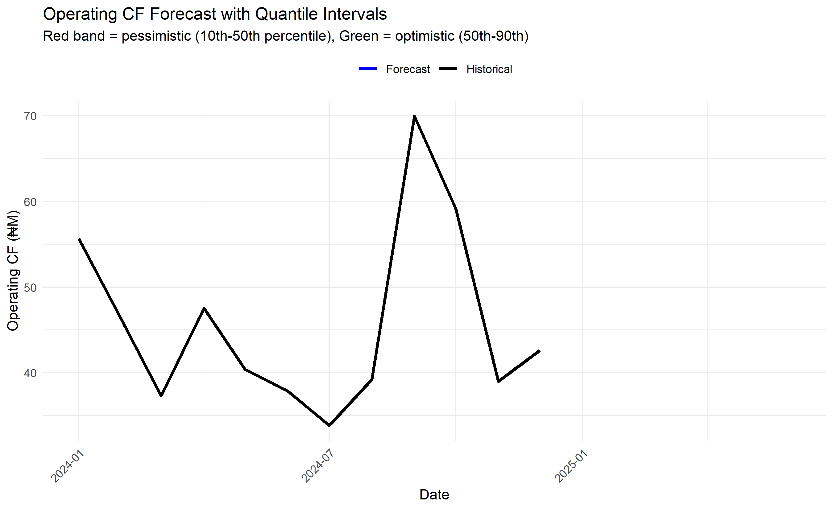
# Visualise: historical data + quantile forecast bands
viz_df_quantile <- bind_rows(
  cf_data |> select(date, operating_cf) |> rename(q50 = operating_cf) |>
    mutate(type = "Historical"),
  fc_quantiles |> mutate(type = "Forecast")
)

ggplot(viz_df_quantile, aes(x = date)) +
  geom_line(aes(y = q50, colour = type), linewidth = 1.2) +
  geom_ribbon(data = fc_quantiles, aes(ymin = q10, ymax = q90),
              alpha = 0.2, fill = "blue") +
  geom_ribbon(data = fc_quantiles, aes(ymin = q10, ymax = q50),
              alpha = 0.15, fill = "red") +
  geom_ribbon(data = fc_quantiles, aes(ymin = q50, ymax = q90),
              alpha = 0.15, fill = "green") +
  scale_colour_manual(values = c("Historical" = "black", "Forecast" = "blue")) +
  labs(title = "Operating CF Forecast with Quantile Intervals",
       subtitle = "Red band = pessimistic (10th-50th percentile), Green = optimistic (50th-90th)",
       x = "Date", y = "Operating CF (₦M)", colour = NULL) +
  theme_minimal() +
  theme(legend.position = "top", axis.text.x = element_text(angle = 45, hjust = 1))

Show code


# Interpretation for treasury
cat("\n\nTreasury Interpretation:\n")
#> 
#> 
#> Treasury Interpretation:
cat("CFO Question: 'With 80% confidence, what is the minimum monthly operating CF?\n")
#> CFO Question: 'With 80% confidence, what is the minimum monthly operating CF?
cat("Answer: Look at the 10th percentile (red band lower edge).\n\n")
#> Answer: Look at the 10th percentile (red band lower edge).

pessimistic <- fc_quantiles |>
  summarise(min_pessimistic = min(q10),
            mean_pessimistic = mean(q10),
            min_optimistic = min(q90),
            mean_optimistic = mean(q90))

cat(sprintf("Minimum Operating CF (10th percentile): ₦%.1fM\n", pessimistic$min_pessimistic))
#> Minimum Operating CF (10th percentile): ₦NaNM
cat(sprintf("Average Operating CF (10th percentile): ₦%.1fM\n", pessimistic$mean_pessimistic))
#> Average Operating CF (10th percentile): ₦NaNM
cat("Recommendation: Plan for ₦ minimum pessimistic as working capital buffer.\n")
#> Recommendation: Plan for ₦ minimum pessimistic as working capital buffer.

Show code

import pandas as pd
import numpy as np
from sklearn.linear_model import QuantileRegressor
from sklearn.preprocessing import StandardScaler
import matplotlib.pyplot as plt

# Build dataset
cf_data = cf_model[['date', 'operating_cf', 'revenue']].dropna().copy()
cf_data['lag_cf'] = cf_data['operating_cf'].shift(1)
cf_data['lag_cf_3'] = cf_data['operating_cf'].shift(3)
cf_data['lag_cf_12'] = cf_data['operating_cf'].shift(12)
cf_data['trend'] = np.arange(len(cf_data))
cf_data['month_sin'] = np.sin(2 * np.pi * cf_data['date'].dt.month / 12)
cf_data['month_cos'] = np.cos(2 * np.pi * cf_data['date'].dt.month / 12)

scaler = StandardScaler()
cf_data['revenue_scaled'] = scaler.fit_transform(cf_data[['revenue']])
cf_data = cf_data.dropna()

# Features
X = cf_data[['lag_cf', 'lag_cf_3', 'lag_cf_12', 'trend', 'month_sin', 'month_cos', 'revenue_scaled']]
y = cf_data['operating_cf']

# Fit quantile regressors
tau_values = [0.1, 0.5, 0.9]
qreg_models = {}

for tau in tau_values:
    qr = QuantileRegressor(quantile=tau, solver='highs')
    qr.fit(X, y)
    qreg_models[tau] = qr
    print(f"\nQuantile {tau:.1%} fitted (R² = {qr.score(X, y):.3f})")

QuantileRegressor(quantile=0.9)

In a Jupyter environment, please rerun this cell to show the HTML representation or trust the notebook.
On GitHub, the HTML representation is unable to render, please try loading this page with nbviewer.org.

Show code


# Forecast
last_idx = len(cf_data) - 1
forecasts = []

for h in range(1, 7):
    # Features for horizon h
    lag_cf_val = cf_data['operating_cf'].iloc[last_idx] if h == 1 else forecasts[-1]['q50']
    month_ahead = (cf_data['date'].iloc[last_idx].month + h) % 12 or 12

    X_new = np.array([[
        lag_cf_val,
        cf_data['lag_cf_3'].iloc[last_idx if h <= 3 else last_idx],
        cf_data['lag_cf_12'].iloc[last_idx - 12 + h] if h <= 12 else cf_data['lag_cf_12'].iloc[-1],
        cf_data['trend'].iloc[last_idx] + h,
        np.sin(2 * np.pi * month_ahead / 12),
        np.cos(2 * np.pi * month_ahead / 12),
        cf_data['revenue_scaled'].iloc[last_idx]
    ]])

    q10 = qreg_models[0.1].predict(X_new)[0]
    q50 = qreg_models[0.5].predict(X_new)[0]
    q90 = qreg_models[0.9].predict(X_new)[0]

    forecasts.append({
        'horizon': h,
        'date': cf_data['date'].iloc[last_idx] + pd.DateOffset(months=h),
        'q10': q10,
        'q50': q50,
        'q90': q90
    })

fc_quantiles = pd.DataFrame(forecasts)

print("\n\n6-Month Forecast with Quantile Intervals (₦M):")
#> 
#> 
#> 6-Month Forecast with Quantile Intervals (₦M):
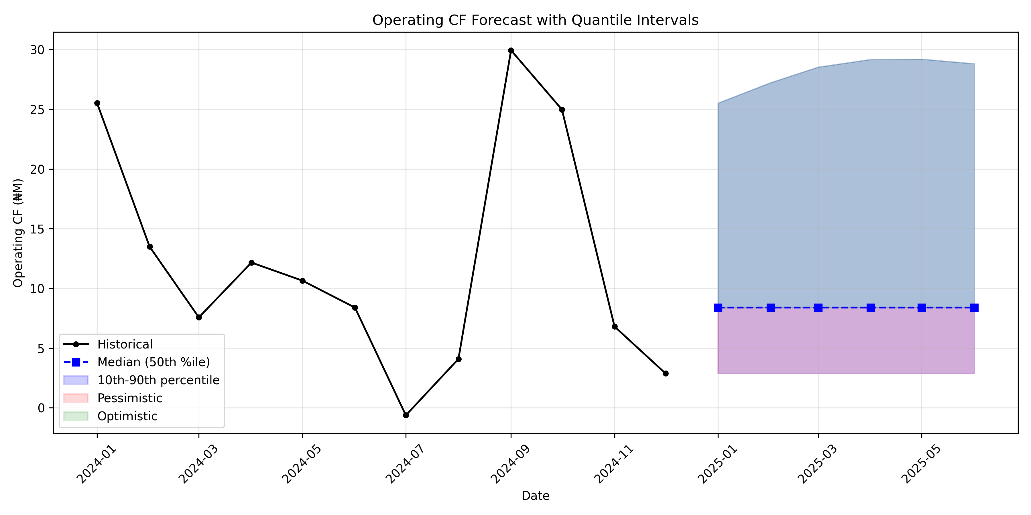
print(fc_quantiles[['horizon', 'date', 'q10', 'q50', 'q90']].round(1))
#>    horizon       date  q10  q50   q90
#> 0        1 2025-01-01  2.9  8.4  25.5
#> 1        2 2025-02-01  2.9  8.4  27.2
#> 2        3 2025-03-01  2.9  8.4  28.5
#> 3        4 2025-04-01  2.9  8.4  29.2
#> 4        5 2025-05-01  2.9  8.4  29.2
#> 5        6 2025-06-01  2.9  8.4  28.8

# Plot
fig, ax = plt.subplots(figsize=(12, 6))
ax.plot(cf_data['date'], cf_data['operating_cf'], 'o-', label='Historical',
        linewidth=1.5, color='black', markersize=4)
ax.plot(fc_quantiles['date'], fc_quantiles['q50'], 's--', label='Median (50th %ile)',
        linewidth=1.5, color='blue')
ax.fill_between(fc_quantiles['date'], fc_quantiles['q10'], fc_quantiles['q90'],
                alpha=0.2, color='blue', label='10th-90th percentile')
ax.fill_between(fc_quantiles['date'], fc_quantiles['q10'], fc_quantiles['q50'],
                alpha=0.15, color='red', label='Pessimistic')
ax.fill_between(fc_quantiles['date'], fc_quantiles['q50'], fc_quantiles['q90'],
                alpha=0.15, color='green', label='Optimistic')
ax.set_xlabel('Date')
ax.set_ylabel('Operating CF (₦M)')
ax.set_title('Operating CF Forecast with Quantile Intervals')
ax.legend()
ax.grid(True, alpha=0.3)
plt.xticks(rotation=45)
#> (array([19723., 19783., 19844., 19905., 19967., 20028., 20089., 20148.,
#>        20209.]), [Text(19723.0, 0, '2024-01'), Text(19783.0, 0, '2024-03'), Text(19844.0, 0, '2024-05'), Text(19905.0, 0, '2024-07'), Text(19967.0, 0, '2024-09'), Text(20028.0, 0, '2024-11'), Text(20089.0, 0, '2025-01'), Text(20148.0, 0, '2025-03'), Text(20209.0, 0, '2025-05')])
plt.tight_layout()
plt.show()

Show code


print("\n\nTreasury Interpretation:")
#> 
#> 
#> Treasury Interpretation:
print(f"Minimum Operating CF (10th %ile): ₦{fc_quantiles['q10'].min():.1f}M")
#> Minimum Operating CF (10th %ile): ₦2.9M
print(f"Mean Operating CF (10th %ile): ₦{fc_quantiles['q10'].mean():.1f}M")
#> Mean Operating CF (10th %ile): ₦2.9M
print("Recommendation: Plan for ₦ minimum as working capital buffer.")
#> Recommendation: Plan for ₦ minimum as working capital buffer.

📝 Section 26.4 Review Questions

Explain the pinball loss function. Why does \(\tau = 0.9\) produce a forecast higher than \(\tau = 0.5\)?
In treasury planning, why is the 10th percentile forecast more useful than the mean forecast?
How would you build a 95% prediction interval from quantile forecasts at \(\tau = 0.025\) and \(\tau = 0.975\)?
If the 10th percentile forecast for months 2-6 is ₦8, 7, 6, 5, 4M, what does this trend suggest about downside risk?
Compare quantile regression to ARIMA prediction intervals. Which is more flexible for capturing asymmetric tail risk?

31.5 Scenario Analysis and Sensitivity: Tornado Charts

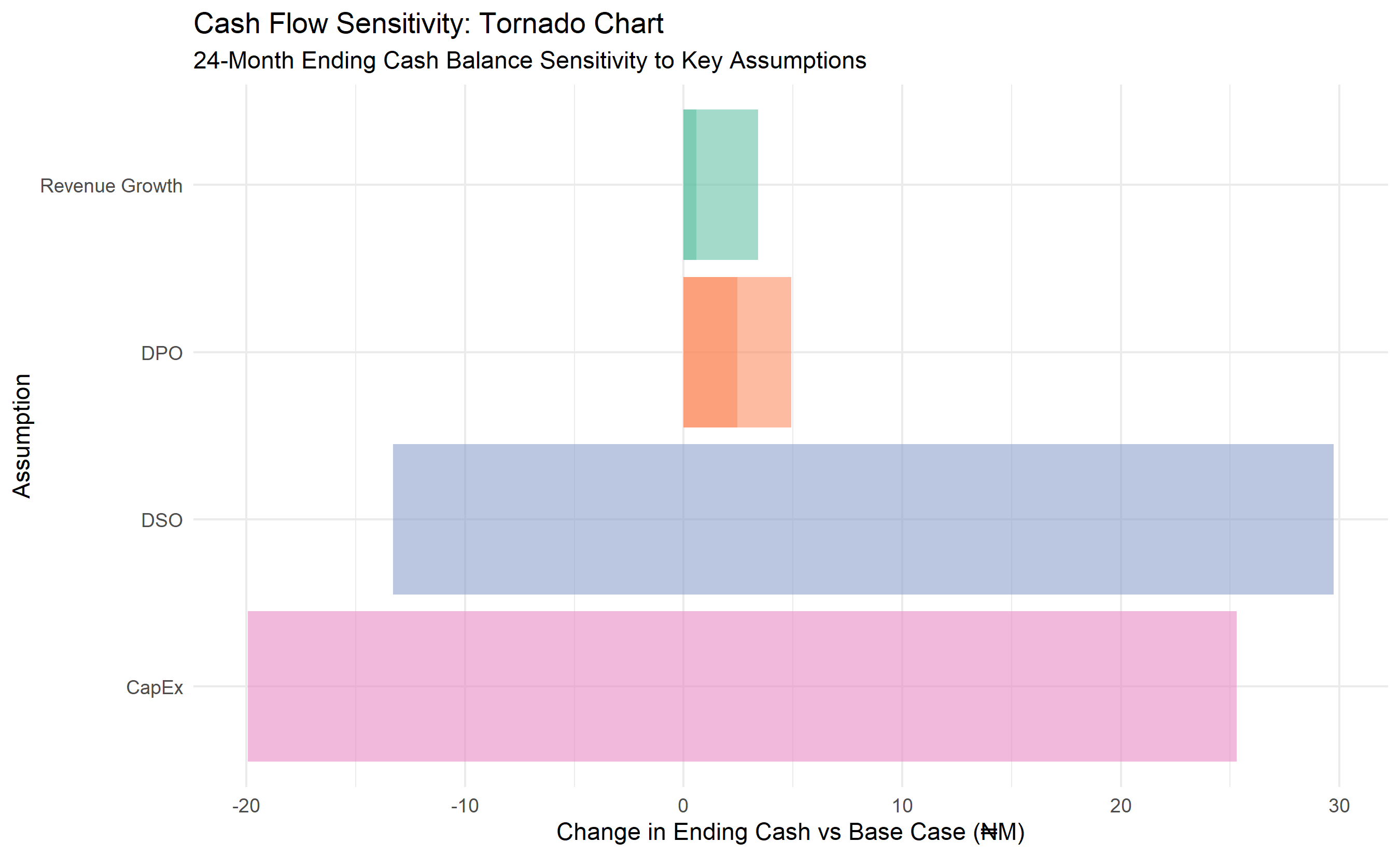
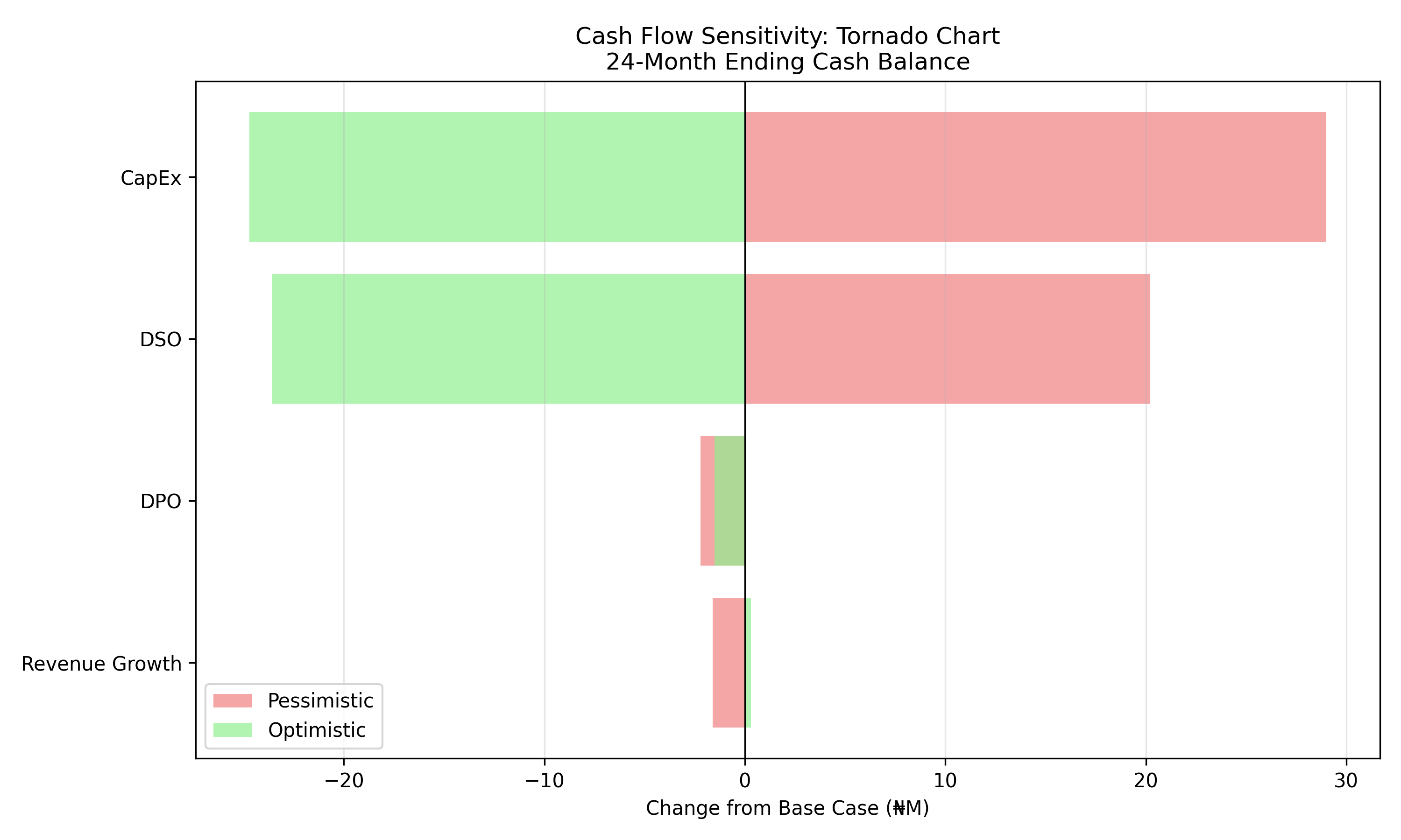
A point forecast assumes base-case assumptions (DSO = 45 days, revenue growth = 10%, etc.). Sensitivity analysis explores how forecast changes if assumptions deviate. A tornado chart ranks which assumptions have the biggest impact.

Methodology: For each key assumption, compute two scenarios: - Optimistic: +20% from base (e.g., if revenue growth = 10%, optimistic = 12%). - Pessimistic: −20% from base (e.g., pessimistic = 8%).

Then forecast 12-month cash balance under each scenario and plot the range.

📘 Theory: Sensitivity Analysis

For a cash flow function \(\text{CF}(x_1, x_2, \ldots, x_k)\), the sensitivity of CF to assumption \(x_i\) is: \[S_i = \frac{\partial \text{CF}}{\partial x_i} \approx \frac{\text{CF}(x_i^{+}) - \text{CF}(x_i^{-})}{x_i^{+} - x_i^{-}}\] where \(x_i^{+}\) and \(x_i^{-}\) are perturbed values. A positive \(S_i > 0\) means CF is positively correlated with \(x_i\).

🔑 Key Formula

Scenario Ranges: \[\text{Range}_i = \text{CF}(x_i^{+}) - \text{CF}(x_i^{-}) = S_i \times (x_i^{+} - x_i^{-})\] Sort ranges in descending order to identify which assumptions drive the most uncertainty. This is a “tornado” because the visual resembles a tornado shape.

Show code

library(tidyverse)
library(ggplot2)

# Run cash flow model with different assumptions
run_cf_model <- function(dso = 45, dpo = 30, revenue_growth_base = 0.08,
                         capex_base = 5) {
  months_future <- 24
  dates <- seq(from = as.Date("2023-01-01"), by = "month", length.out = months_future)

  base_revenue <- 50
  trend_factor <- seq(1, 1 + revenue_growth_base * 2, length.out = months_future)
  seasonal <- rep(c(0.9, 0.95, 1.0, 0.95, 0.95, 1.0, 1.2, 1.3, 1.0, 0.95, 1.1, 1.2),
                  length.out = months_future)

  revenue <- base_revenue * trend_factor * seasonal + rnorm(months_future, 0, 2)
  revenue <- pmax(revenue, 15)

  cogs <- revenue * 0.55
  opex <- revenue * 0.25

  cf_model <- data.frame(
    month = 1:months_future,
    date = dates,
    revenue = revenue,
    cogs = cogs,
    opex = opex
  ) |>
    mutate(
      lag_revenue = lag(revenue, 1),
      lag_revenue_2 = lag(revenue, 2),
      collections = revenue * (30 - dso) / 30 +
                    ifelse(is.na(lag_revenue), 0, lag_revenue * dso / 30),
      lag_cogs = lag(cogs, 1),
      supplier_payments = ifelse(is.na(lag_cogs), cogs * 0.5, lag_cogs),
      payroll_and_opex = opex,
      capex = capex_base,
      loan_repayment = c(3, 0, 0) %*% t(rep(1, 8)) |> c(),
      tax_payment = 0,
      operating_cf = collections - supplier_payments - payroll_and_opex,
      free_cf = operating_cf - capex - loan_repayment,
      beginning_cash = c(50, rep(NA_real_, months_future - 1)),
      ending_cash = NA_real_
    )

  cf_model$ending_cash[1] <- cf_model$beginning_cash[1] + cf_model$free_cf[1]
  for (i in 2:nrow(cf_model)) {
    cf_model$beginning_cash[i] <- cf_model$ending_cash[i - 1]
    cf_model$ending_cash[i] <- cf_model$beginning_cash[i] + cf_model$free_cf[i]
  }

  return(cf_model)
}

# Base case
cf_base <- run_cf_model()

# Sensitivity scenarios
assumptions <- list(
  list(name = "DSO", base = 45, vars = c(36, 54)),
  list(name = "DPO", base = 30, vars = c(24, 36)),
  list(name = "Revenue Growth", base = 0.08, vars = c(0.064, 0.096)),
  list(name = "CapEx", base = 5, vars = c(4, 6))
)

sensitivity_results <- data.frame()

for (assumption in assumptions) {
  name <- assumption$name
  base_val <- assumption$base
  var_pessimistic <- assumption$vars[1]
  var_optimistic <- assumption$vars[2]

  # Run pessimistic and optimistic
  if (name == "DSO") {
    cf_pess <- run_cf_model(dso = var_pessimistic)
    cf_opt <- run_cf_model(dso = var_optimistic)
  } else if (name == "DPO") {
    cf_pess <- run_cf_model(dpo = var_pessimistic)
    cf_opt <- run_cf_model(dpo = var_optimistic)
  } else if (name == "Revenue Growth") {
    cf_pess <- run_cf_model(revenue_growth_base = var_pessimistic)
    cf_opt <- run_cf_model(revenue_growth_base = var_optimistic)
  } else if (name == "CapEx") {
    cf_pess <- run_cf_model(capex_base = var_pessimistic)
    cf_opt <- run_cf_model(capex_base = var_optimistic)
  }

  # Extract 24-month ending cash
  cash_pess <- cf_pess$ending_cash[24]
  cash_opt <- cf_opt$ending_cash[24]
  cash_base <- cf_base$ending_cash[24]

  sensitivity_results <- rbind(sensitivity_results, data.frame(
    assumption = name,
    pessimistic = cash_pess,
    optimistic = cash_opt,
    range = cash_opt - cash_pess
  ))
}

# Sort by range (tornado order)
sensitivity_results <- sensitivity_results |>
  arrange(desc(range)) |>
  mutate(assumption = factor(assumption, levels = unique(assumption)))

cat("24-Month Ending Cash Sensitivity Analysis (₦M)\n\n")
#> 24-Month Ending Cash Sensitivity Analysis (₦M)
print(sensitivity_results |>
        mutate(across(where(is.numeric), round, 1)))
#>       assumption pessimistic optimistic range
#> 1 Revenue Growth        94.0       96.8   2.8
#> 2            DPO        95.8       98.3   2.5
#> 3            DSO       123.1       80.1 -43.0
#> 4          CapEx       118.7       73.4 -45.2

# Tornado chart
ggplot(sensitivity_results, aes(x = reorder(assumption, range), fill = assumption)) +
  geom_col(aes(y = pessimistic - cf_base$ending_cash[24]), alpha = 0.6) +
  geom_col(aes(y = optimistic - cf_base$ending_cash[24]), alpha = 0.6) +
  coord_flip() +
  scale_fill_brewer(palette = "Set2") +
  labs(title = "Cash Flow Sensitivity: Tornado Chart",
       subtitle = "24-Month Ending Cash Balance Sensitivity to Key Assumptions",
       x = "Assumption", y = "Change in Ending Cash vs Base Case (₦M)", fill = NULL) +
  theme_minimal() +
  theme(legend.position = "none")

Show code


# Create a summary recommendation table
cat("\n\nManagement Summary:\n")
#> 
#> 
#> Management Summary:
cat("Base Case 24-Month Ending Cash: ₦", round(cf_base$ending_cash[24], 1), "M\n\n")
#> Base Case 24-Month Ending Cash: ₦ 93.4 M

cat("Assumption Ranking by Impact (most to least sensitive):\n")
#> Assumption Ranking by Impact (most to least sensitive):
for (i in 1:nrow(sensitivity_results)) {
  r <- sensitivity_results[i, ]
  pct_impact <- (r$range / cf_base$ending_cash[24]) * 100
  cat(sprintf("%d. %s: ±₦%.1fM (±%.0f%% of base)\n",
              i, r$assumption, r$range / 2, pct_impact / 2))
}
#> 1. Revenue Growth: ±₦1.4M (±2% of base)
#> 2. DPO: ±₦1.2M (±1% of base)
#> 3. DSO: ±₦-21.5M (±-23% of base)
#> 4. CapEx: ±₦-22.6M (±-24% of base)

Show code

import pandas as pd
import numpy as np
import matplotlib.pyplot as plt

def run_cf_model(dso=45, dpo=30, revenue_growth_base=0.08, capex_base=5):
    months_future = 24
    dates = pd.date_range(start='2023-01-01', periods=months_future, freq='MS')

    base_revenue = 50
    trend_factor = np.linspace(1, 1 + revenue_growth_base * 2, months_future)
    seasonal = np.tile([0.9, 0.95, 1.0, 0.95, 0.95, 1.0,
                        1.2, 1.3, 1.0, 0.95, 1.1, 1.2], 2)[:months_future]
    revenue = base_revenue * trend_factor * seasonal + np.random.normal(0, 2, months_future)
    revenue = np.maximum(revenue, 15)

    cogs = revenue * 0.55
    opex = revenue * 0.25

    cf = pd.DataFrame({
        'date': dates,
        'revenue': revenue,
        'cogs': cogs,
        'opex': opex
    })

    cf['lag_revenue'] = cf['revenue'].shift(1)
    cf['collections'] = (cf['revenue'] * (30 - dso) / 30 +
                         cf['lag_revenue'].fillna(0) * dso / 30)
    cf['lag_cogs'] = cf['cogs'].shift(1)
    cf['supplier_payments'] = cf['lag_cogs'].fillna(cf['cogs'] * 0.5)
    cf['payroll_and_opex'] = cf['opex']
    cf['capex'] = capex_base
    cf['loan_repayment'] = np.tile([3, 0, 0], 8)[:months_future]
    cf['tax_payment'] = 0

    cf['operating_cf'] = cf['collections'] - cf['supplier_payments'] - cf['payroll_and_opex']
    cf['free_cf'] = cf['operating_cf'] - cf['capex'] - cf['loan_repayment']
    cf['beginning_cash'] = 50.0
    cf['ending_cash'] = 0.0
    cf.loc[0, 'ending_cash'] = cf.loc[0, 'beginning_cash'] + cf.loc[0, 'free_cf']
    for i in range(1, len(cf)):
        cf.loc[i, 'beginning_cash'] = cf.loc[i-1, 'ending_cash']
        cf.loc[i, 'ending_cash'] = cf.loc[i, 'beginning_cash'] + cf.loc[i, 'free_cf']
    return cf

# Base case
np.random.seed(111)
cf_base = run_cf_model()

# Sensitivity
assumptions = {
    'DSO': {'base': 45, 'range': [36, 54], 'param': 'dso'},
    'DPO': {'base': 30, 'range': [24, 36], 'param': 'dpo'},
    'Revenue Growth': {'base': 0.08, 'range': [0.064, 0.096], 'param': 'rev'},
    'CapEx': {'base': 5, 'range': [4, 6], 'param': 'capex'}
}

sensitivity_results = []

for name, spec in assumptions.items():
    var_pess, var_opt = spec['range']
    param = spec['param']

    if param == 'dso':
        cf_pess = run_cf_model(dso=var_pess)
        cf_opt = run_cf_model(dso=var_opt)
    elif param == 'dpo':
        cf_pess = run_cf_model(dpo=var_pess)
        cf_opt = run_cf_model(dpo=var_opt)
    elif param == 'rev':
        cf_pess = run_cf_model(revenue_growth_base=var_pess)
        cf_opt = run_cf_model(revenue_growth_base=var_opt)
    elif param == 'capex':
        cf_pess = run_cf_model(capex_base=var_pess)
        cf_opt = run_cf_model(capex_base=var_opt)

    cash_pess = cf_pess['ending_cash'].iloc[-1]
    cash_opt = cf_opt['ending_cash'].iloc[-1]
    cash_range = cash_opt - cash_pess

    sensitivity_results.append({
        'Assumption': name,
        'Pessimistic': round(cash_pess, 1),
        'Optimistic': round(cash_opt, 1),
        'Range': round(cash_range, 1)
    })

sensitivity_df = pd.DataFrame(sensitivity_results).sort_values('Range', ascending=False)

print("24-Month Ending Cash Sensitivity Analysis (₦M)\n")
#> 24-Month Ending Cash Sensitivity Analysis (₦M)
print(sensitivity_df.to_string(index=False))
#>     Assumption  Pessimistic  Optimistic  Range
#> Revenue Growth         95.4        97.3    2.0
#>            DPO         94.8        95.5    0.7
#>            DSO        117.2        73.4  -43.8
#>          CapEx        126.0        72.3  -53.7

# Tornado chart
fig, ax = plt.subplots(figsize=(10, 6))
y_pos = np.arange(len(sensitivity_df))
cash_base = cf_base['ending_cash'].iloc[-1]

# Pessimistic bars (negative)
pess_offset = sensitivity_df['Pessimistic'] - cash_base
opt_offset = sensitivity_df['Optimistic'] - cash_base

ax.barh(y_pos, pess_offset, label='Pessimistic', color='lightcoral', alpha=0.7)
ax.barh(y_pos, opt_offset, label='Optimistic', color='lightgreen', alpha=0.7)

ax.set_yticks(y_pos)
ax.set_yticklabels(sensitivity_df['Assumption'])
ax.set_xlabel('Change from Base Case (₦M)')
ax.set_title('Cash Flow Sensitivity: Tornado Chart\n24-Month Ending Cash Balance')
ax.axvline(x=0, color='black', linestyle='-', linewidth=0.8)
ax.legend()
ax.grid(True, alpha=0.3, axis='x')
plt.tight_layout()
plt.show()

Show code


print(f"\n\nBase Case 24-Month Ending Cash: ₦{cash_base:.1f}M\n")
#> 
#> 
#> Base Case 24-Month Ending Cash: ₦97.0M
print("Assumption Ranking by Impact:")
#> Assumption Ranking by Impact:
for i, row in sensitivity_df.iterrows():
    pct = (row['Range'] / cash_base) * 100
    print(f"{i+1}. {row['Assumption']}: ±₦{row['Range']/2:.1f}M (±{pct/2:.0f}%)")
#> 3. Revenue Growth: ±₦1.0M (±1%)
#> 2. DPO: ±₦0.3M (±0%)
#> 1. DSO: ±₦-21.9M (±-23%)
#> 4. CapEx: ±₦-26.9M (±-28%)

📝 Section 26.5 Review Questions

In a tornado chart, why do assumptions with larger ranges get higher priority for monitoring?
If revenue growth has the largest impact on ending cash, what strategies would you pursue to reduce that risk?
How would you set monitoring thresholds based on sensitivity analysis? (e.g., “If DSO exceeds X days, trigger action”)
Explain the difference between sensitivity analysis and scenario analysis. When would you use each?
If pessimistic DSO = ₦5M and optimistic DSO = ₦25M, but the base case ending cash is ₦50M, is DSO risk acceptable?

31.6 Monte Carlo Simulation: Quantifying Tail Risk

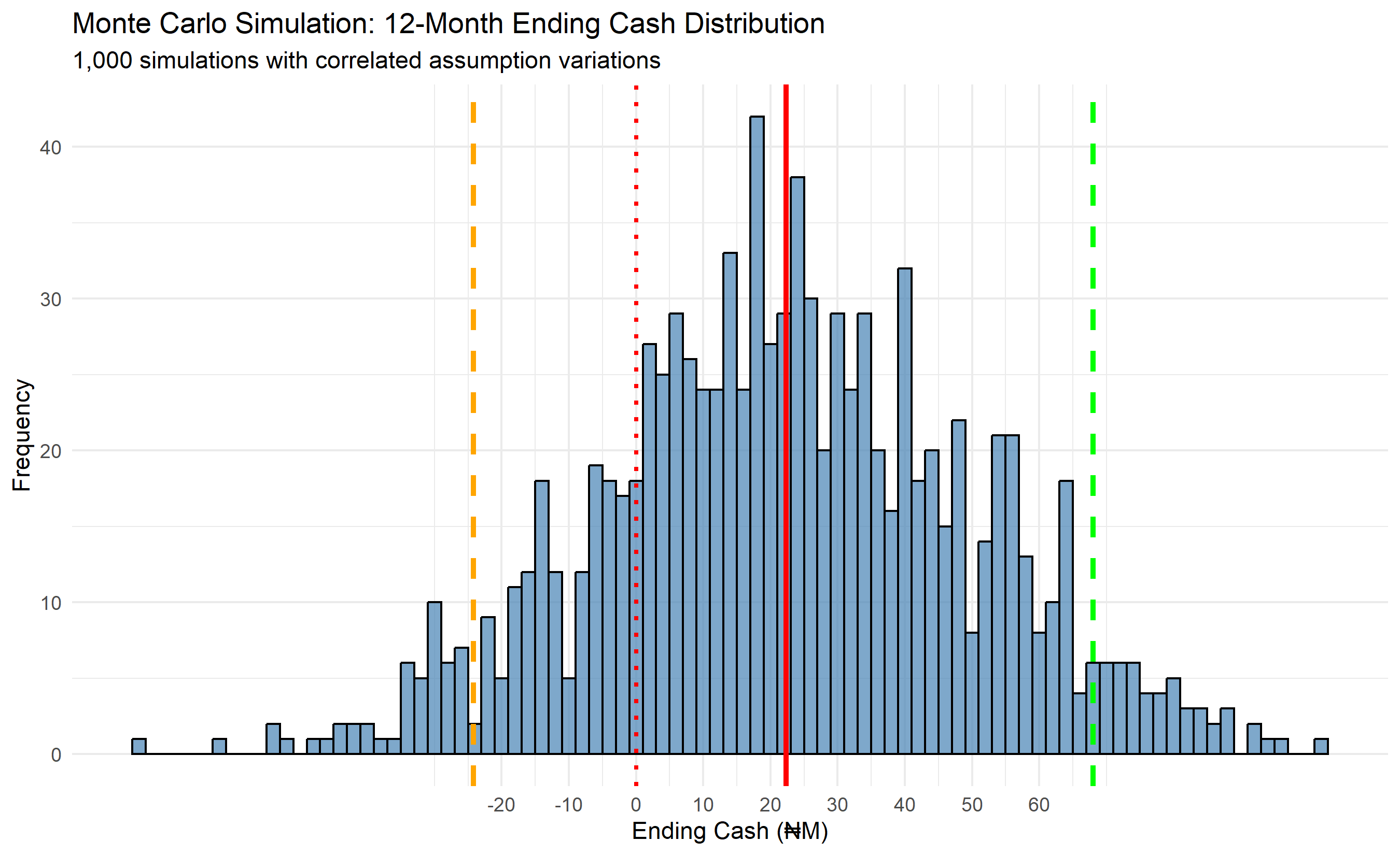
Sensitivity analysis assumes independence: only one assumption varies at a time. In reality, DSO, revenue, and costs are often correlated. When revenue drops (recession), DSO also increases (customers pay slower). Monte Carlo simulation samples all assumptions simultaneously from probability distributions and runs the cash flow model thousands of times, generating a distribution of outcomes.

The results show not just the mean and standard deviation but also tail risk: the 5th percentile (downside risk) and 95th percentile (upside potential).

📘 Theory: Monte Carlo for Cash Flow Risk

Given assumptions \((x_1, x_2, \ldots, x_k)\) drawn from distributions \(X_1, X_2, \ldots, X_k\), run the cash flow model \(N\) times (typically 500–10,000): 1. Sample \(\mathbf{x}^{(i)} = (x_1^{(i)}, \ldots, x_k^{(i)})\) from joint distribution. 2. Run CF model with \(\mathbf{x}^{(i)}\) to obtain ending cash \(C^{(i)}\). 3. Repeat for \(i = 1, \ldots, N\). 4. Estimate percentiles, variance, and probability of cash shortfall from the sample \(\{C^{(1)}, \ldots, C^{(N)}\}\).

🔑 Key Formula

Value-at-Risk (VaR) from Monte Carlo: \[\text{VaR}_{95\%} = \text{Percentile}_{5}\{C^{(1)}, \ldots, C^{(N)}\}\] The 5th percentile of simulated ending cash balances. Means there’s a 5% probability of cash falling below this level.

Show code

library(tidyverse)
library(ggplot2)

# Monte Carlo simulation for cash flow
monte_carlo_cf <- function(n_simulations = 1000, seed = 222) {
  set.seed(seed)

  months_forecast <- 12
  dates <- seq(from = as.Date("2024-01-01"), by = "month", length.out = months_forecast)

  # Distribution assumptions
  dso_dist <- rnorm(n_simulations, mean = 45, sd = 10)  # 45±10 days
  dpo_dist <- rnorm(n_simulations, mean = 30, sd = 8)   # 30±8 days
  revenue_growth <- rnorm(n_simulations, mean = 0.08, sd = 0.03)  # 8%±3%
  capex_dist <- rnorm(n_simulations, mean = 5, sd = 1.5)  # 5±1.5M

  results <- data.frame()

  for (sim in 1:n_simulations) {
    dso <- pmax(20, dso_dist[sim])  # Floor at 20 days
    dpo <- pmax(15, dpo_dist[sim])  # Floor at 15 days
    rev_growth <- pmax(0.01, revenue_growth[sim])  # Floor at 1%
    capex <- pmax(2, capex_dist[sim])  # Floor at 2M

    # Generate 12-month forecast
    base_revenue <- 50
    trend <- seq(1, 1 + rev_growth * 1, length.out = months_forecast)
    seasonal <- c(0.95, 0.95, 1.0, 0.95, 0.95, 1.0, 1.2, 1.3, 1.0, 0.95, 1.1, 1.2)

    revenue <- base_revenue * trend * seasonal + rnorm(months_forecast, 0, 2)
    revenue <- pmax(revenue, 15)

    cogs <- revenue * 0.55
    opex <- revenue * 0.25

    cf_data <- data.frame(
      month = 1:months_forecast,
      revenue = revenue,
      cogs = cogs,
      opex = opex
    ) |>
      mutate(
        lag_revenue = lag(revenue, 1),
        collections = revenue * (30 - dso) / 30 +
                      ifelse(is.na(lag_revenue), 0, lag_revenue * dso / 30),
        lag_cogs = lag(cogs, 1),
        supplier_payments = ifelse(is.na(lag_cogs), cogs * 0.5, lag_cogs),
        payroll_and_opex = opex,
        capex = capex,
        loan_repayment = 2,
        operating_cf = collections - supplier_payments - payroll_and_opex,
        free_cf = operating_cf - capex - loan_repayment,
        beginning_cash = 50
      )

    for (i in 2:nrow(cf_data)) {
      cf_data$beginning_cash[i] <- cf_data$beginning_cash[i - 1] + cf_data$free_cf[i - 1]
    }

    cf_data <- cf_data |>
      mutate(ending_cash = beginning_cash + free_cf)

    # Store 12-month ending cash
    results <- rbind(results, data.frame(
      simulation = sim,
      ending_cash_12m = cf_data$ending_cash[12],
      min_cash = min(cf_data$ending_cash),
      revenue_total = sum(cf_data$revenue),
      dso = dso,
      dpo = dpo
    ))
  }

  return(results)
}

# Run simulation
mc_results <- monte_carlo_cf(n_simulations = 1000)

# Summary statistics
cat("Monte Carlo Simulation Results (1,000 runs, 12-month forecast)\n\n")
#> Monte Carlo Simulation Results (1,000 runs, 12-month forecast)

summary_stats <- mc_results |>
  summarise(
    mean_cash = mean(ending_cash_12m),
    median_cash = median(ending_cash_12m),
    std_cash = sd(ending_cash_12m),
    p5_cash = quantile(ending_cash_12m, 0.05),
    p25_cash = quantile(ending_cash_12m, 0.25),
    p75_cash = quantile(ending_cash_12m, 0.75),
    p95_cash = quantile(ending_cash_12m, 0.95),
    min_cash = min(ending_cash_12m),
    max_cash = max(ending_cash_12m),
    prob_negative = mean(ending_cash_12m < 0),
    prob_shortfall_10m = mean(ending_cash_12m < 10)
  )

cat("12-Month Ending Cash Distribution (₦M):\n")
#> 12-Month Ending Cash Distribution (₦M):
for (col in names(summary_stats)) {
  val <- summary_stats[[col]]
  if (col == "prob_negative" || col == "prob_shortfall_10m") {
    cat(sprintf("%s: %.2f%%\n", col, val * 100))
  } else {
    cat(sprintf("%s: %.1f\n", col, val))
  }
}
#> mean_cash: 22.3
#> median_cash: 22.1
#> std_cash: 27.5
#> p5_cash: -24.2
#> p25_cash: 4.1
#> p75_cash: 40.7
#> p95_cash: 68.0
#> min_cash: -73.8
#> max_cash: 102.6
#> prob_negative: 19.70%
#> prob_shortfall_10m: 32.70%

cat("\n\nTreasury Insights:\n")
#> 
#> 
#> Treasury Insights:
cat(sprintf("Base Case (Mean): ₦%.1fM\n", summary_stats$mean_cash))
#> Base Case (Mean): ₦22.3M
cat(sprintf("Downside Risk (5th percentile): ₦%.1fM\n", summary_stats$p5_cash))
#> Downside Risk (5th percentile): ₦-24.2M
cat(sprintf("Upside Potential (95th percentile): ₦%.1fM\n", summary_stats$p95_cash))
#> Upside Potential (95th percentile): ₦68.0M
cat(sprintf("Probability of Negative Cash: %.1f%%\n", summary_stats$prob_negative * 100))
#> Probability of Negative Cash: 19.7%
cat(sprintf("Probability of Cash < ₦10M: %.1f%%\n", summary_stats$prob_shortfall_10m * 100))
#> Probability of Cash < ₦10M: 32.7%

# Distribution histogram
ggplot(mc_results, aes(x = ending_cash_12m)) +
  geom_histogram(binwidth = 2, fill = "steelblue", alpha = 0.7, color = "black") +
  geom_vline(xintercept = summary_stats$mean_cash, colour = "red", linetype = "solid",
             linewidth = 1.2, label = "Mean") +
  geom_vline(xintercept = summary_stats$p5_cash, colour = "orange", linetype = "dashed",
             linewidth = 1.2, label = "5th percentile") +
  geom_vline(xintercept = summary_stats$p95_cash, colour = "green", linetype = "dashed",
             linewidth = 1.2, label = "95th percentile") +
  geom_vline(xintercept = 0, colour = "red", linetype = "dotted",
             linewidth = 1, label = "Zero cash") +
  scale_x_continuous(breaks = seq(-20, 60, by = 10)) +
  labs(title = "Monte Carlo Simulation: 12-Month Ending Cash Distribution",
       subtitle = "1,000 simulations with correlated assumption variations",
       x = "Ending Cash (₦M)", y = "Frequency") +
  theme_minimal() +
  theme(legend.position = "top")

Show code


# Q-Q plot to check normality
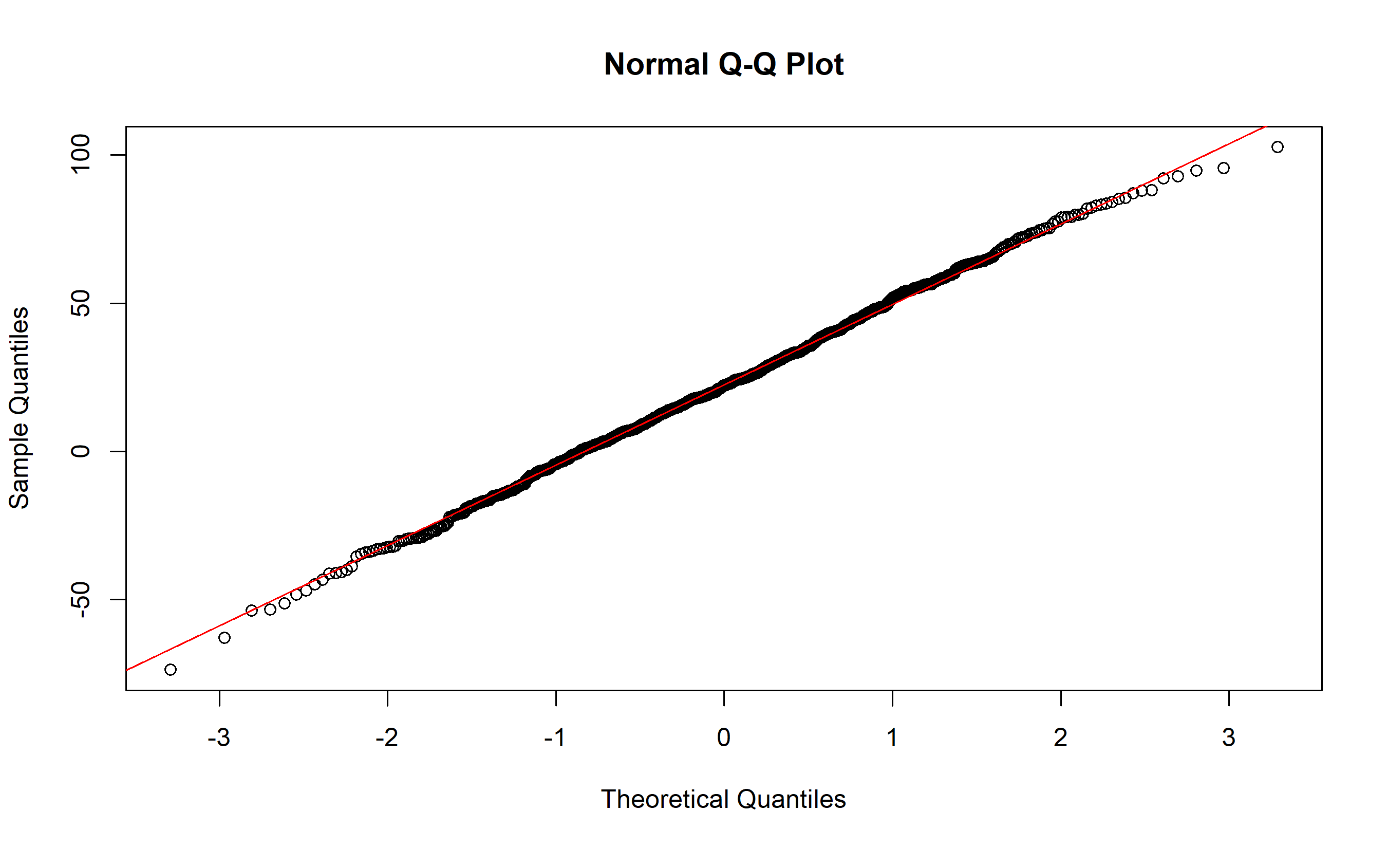
qqnorm(mc_results$ending_cash_12m)
qqline(mc_results$ending_cash_12m, col = "red")

Show code

import numpy as np
import pandas as pd
import matplotlib.pyplot as plt
from scipy import stats

def monte_carlo_cf(n_simulations=1000, seed=222):
    np.random.seed(seed)

    months_forecast = 12

    # Sample distributions
    dso_dist = np.random.normal(45, 10, n_simulations)
    dpo_dist = np.random.normal(30, 8, n_simulations)
    revenue_growth = np.random.normal(0.08, 0.03, n_simulations)
    capex_dist = np.random.normal(5, 1.5, n_simulations)

    results = []

    for sim in range(n_simulations):
        dso = max(20, dso_dist[sim])
        dpo = max(15, dpo_dist[sim])
        rev_growth = max(0.01, revenue_growth[sim])
        capex = max(2, capex_dist[sim])

        base_revenue = 50
        trend = np.linspace(1, 1 + rev_growth, months_forecast)
        seasonal = np.array([0.95, 0.95, 1.0, 0.95, 0.95, 1.0,
                            1.2, 1.3, 1.0, 0.95, 1.1, 1.2])
        revenue = base_revenue * trend * seasonal + np.random.normal(0, 2, months_forecast)
        revenue = np.maximum(revenue, 15)

        cogs = revenue * 0.55
        opex = revenue * 0.25

        cf_data = pd.DataFrame({
            'revenue': revenue,
            'cogs': cogs,
            'opex': opex
        })

        cf_data['lag_revenue'] = cf_data['revenue'].shift(1)
        cf_data['collections'] = (cf_data['revenue'] * (30 - dso) / 30 +
                                  cf_data['lag_revenue'].fillna(0) * dso / 30)
        cf_data['lag_cogs'] = cf_data['cogs'].shift(1)
        cf_data['supplier_payments'] = cf_data['lag_cogs'].fillna(cf_data['cogs'] * 0.5)
        cf_data['payroll_and_opex'] = cf_data['opex']
        cf_data['capex'] = capex
        cf_data['loan_repayment'] = 2

        cf_data['operating_cf'] = (cf_data['collections'] - cf_data['supplier_payments'] -
                                   cf_data['payroll_and_opex'])
        cf_data['free_cf'] = cf_data['operating_cf'] - cf_data['capex'] - cf_data['loan_repayment']
        cf_data['beginning_cash'] = 50.0
        cf_data['ending_cash'] = 0.0
        cf_data.loc[0, 'ending_cash'] = cf_data.loc[0, 'beginning_cash'] + cf_data.loc[0, 'free_cf']
        for i in range(1, len(cf_data)):
            cf_data.loc[i, 'beginning_cash'] = cf_data.loc[i-1, 'ending_cash']
            cf_data.loc[i, 'ending_cash'] = cf_data.loc[i, 'beginning_cash'] + cf_data.loc[i, 'free_cf']

        results.append({
            'simulation': sim,
            'ending_cash_12m': cf_data['ending_cash'].iloc[-1],
            'min_cash': cf_data['ending_cash'].min(),
            'revenue_total': cf_data['revenue'].sum(),
            'dso': dso,
            'dpo': dpo
        })

    return pd.DataFrame(results)

mc_results = monte_carlo_cf(n_simulations=1000)

print("Monte Carlo Simulation Results (1,000 runs, 12-month forecast)\n")
#> Monte Carlo Simulation Results (1,000 runs, 12-month forecast)
print("12-Month Ending Cash Distribution (₦M):")
#> 12-Month Ending Cash Distribution (₦M):
print(f"Mean: {mc_results['ending_cash_12m'].mean():.1f}")
#> Mean: 22.0
print(f"Median: {mc_results['ending_cash_12m'].median():.1f}")
#> Median: 23.0
print(f"Std Dev: {mc_results['ending_cash_12m'].std():.1f}")
#> Std Dev: 27.5
print(f"5th %ile: {mc_results['ending_cash_12m'].quantile(0.05):.1f}")
#> 5th %ile: -25.9
print(f"25th %ile: {mc_results['ending_cash_12m'].quantile(0.25):.1f}")
#> 25th %ile: 3.7
print(f"75th %ile: {mc_results['ending_cash_12m'].quantile(0.75):.1f}")
#> 75th %ile: 39.9
print(f"95th %ile: {mc_results['ending_cash_12m'].quantile(0.95):.1f}")
#> 95th %ile: 65.8
print(f"Min: {mc_results['ending_cash_12m'].min():.1f}")
#> Min: -72.5
print(f"Max: {mc_results['ending_cash_12m'].max():.1f}")
#> Max: 95.4

prob_neg = (mc_results['ending_cash_12m'] < 0).sum() / len(mc_results) * 100
prob_short = (mc_results['ending_cash_12m'] < 10).sum() / len(mc_results) * 100
print(f"\nProbability of Negative Cash: {prob_neg:.2f}%")
#> 
#> Probability of Negative Cash: 21.10%
print(f"Probability of Cash < ₦10M: {prob_short:.2f}%")
#> Probability of Cash < ₦10M: 31.50%

# Histogram
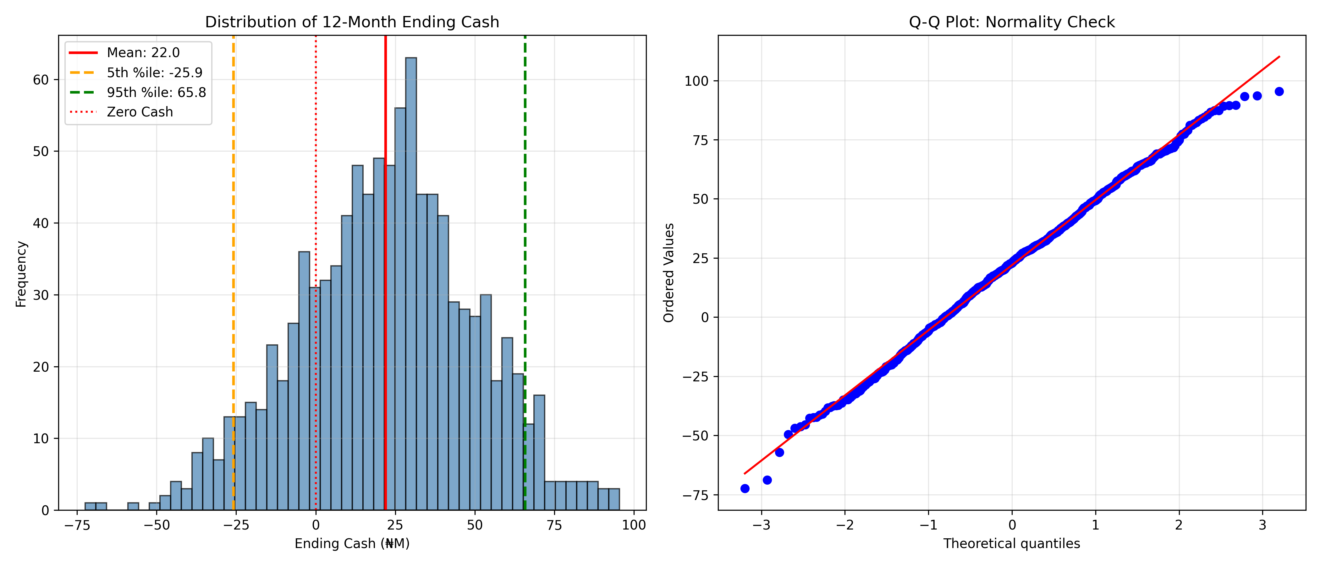
fig, (ax1, ax2) = plt.subplots(1, 2, figsize=(14, 6))

ax1.hist(mc_results['ending_cash_12m'], bins=50, color='steelblue', alpha=0.7, edgecolor='black')
ax1.axvline(mc_results['ending_cash_12m'].mean(), color='red', linestyle='-',
            linewidth=2, label=f"Mean: {mc_results['ending_cash_12m'].mean():.1f}")
ax1.axvline(mc_results['ending_cash_12m'].quantile(0.05), color='orange', linestyle='--',
            linewidth=2, label=f"5th %ile: {mc_results['ending_cash_12m'].quantile(0.05):.1f}")
ax1.axvline(mc_results['ending_cash_12m'].quantile(0.95), color='green', linestyle='--',
            linewidth=2, label=f"95th %ile: {mc_results['ending_cash_12m'].quantile(0.95):.1f}")
ax1.axvline(0, color='red', linestyle=':', linewidth=1.5, label='Zero Cash')
ax1.set_xlabel('Ending Cash (₦M)')
ax1.set_ylabel('Frequency')
ax1.set_title('Distribution of 12-Month Ending Cash')
ax1.legend()
ax1.grid(True, alpha=0.3)

# Q-Q plot
stats.probplot(mc_results['ending_cash_12m'], dist="norm", plot=ax2)
#> ((array([-3.19758950e+00, -2.93237785e+00, -2.78437841e+00, -2.67999560e+00,
#>        -2.59855946e+00, -2.53139899e+00, -2.47402263e+00, -2.42379214e+00,
#>        -2.37902149e+00, -2.33856546e+00, -2.30160949e+00, -2.26755284e+00,
#>        -2.23593934e+00, -2.20641415e+00, -2.17869564e+00, -2.15255643e+00,
#>        -2.12781017e+00, -2.10430217e+00, -2.08190261e+00, -2.06050135e+00,
#>        -2.04000420e+00, -2.02032992e+00, -2.00140792e+00, -1.98317650e+00,
#>        -1.96558137e+00, -1.94857451e+00, -1.93211325e+00, -1.91615948e+00,
#>        -1.90067901e+00, -1.88564107e+00, -1.87101783e+00, -1.85678408e+00,
#>        -1.84291686e+00, -1.82939524e+00, -1.81620005e+00, -1.80331371e+00,
#>        -1.79072004e+00, -1.77840415e+00, -1.76635224e+00, -1.75455157e+00,
#>        -1.74299028e+00, -1.73165738e+00, -1.72054262e+00, -1.70963644e+00,
#>        -1.69892989e+00, -1.68841463e+00, -1.67808281e+00, -1.66792707e+00,
#>        -1.65794051e+00, -1.64811661e+00, -1.63844924e+00, -1.62893261e+00,
#>        -1.61956127e+00, -1.61033003e+00, -1.60123402e+00, -1.59226859e+00,
#>        -1.58342935e+00, -1.57471213e+00, -1.56611295e+00, -1.55762804e+00,
#>        -1.54925381e+00, -1.54098684e+00, -1.53282387e+00, -1.52476177e+00,
#>        -1.51679758e+00, -1.50892845e+00, -1.50115166e+00, -1.49346462e+00,
#>        -1.48586482e+00, -1.47834989e+00, -1.47091753e+00, -1.46356555e+00,
#>        -1.45629184e+00, -1.44909437e+00, -1.44197119e+00, -1.43492043e+00,
#>        -1.42794030e+00, -1.42102906e+00, -1.41418503e+00, -1.40740661e+00,
#>        -1.40069224e+00, -1.39404044e+00, -1.38744975e+00, -1.38091878e+00,
#>        -1.37444619e+00, -1.36803067e+00, -1.36167098e+00, -1.35536588e+00,
#>        -1.34911421e+00, -1.34291482e+00, -1.33676663e+00, -1.33066855e+00,
#>        -1.32461956e+00, -1.31861865e+00, -1.31266485e+00, -1.30675722e+00,
#>        -1.30089485e+00, -1.29507686e+00, -1.28930237e+00, -1.28357055e+00,
#>        -1.27788060e+00, -1.27223172e+00, -1.26662315e+00, -1.26105415e+00,
#>        -1.25552398e+00, -1.25003194e+00, -1.24457735e+00, -1.23915954e+00,
#>        -1.23377786e+00, -1.22843168e+00, -1.22312038e+00, -1.21784337e+00,
#>        -1.21260004e+00, -1.20738985e+00, -1.20221223e+00, -1.19706664e+00,
#>        -1.19195255e+00, -1.18686944e+00, -1.18181682e+00, -1.17679419e+00,
#>        -1.17180107e+00, -1.16683699e+00, -1.16190151e+00, -1.15699416e+00,
#>        -1.15211453e+00, -1.14726217e+00, -1.14243667e+00, -1.13763763e+00,
#>        -1.13286465e+00, -1.12811734e+00, -1.12339532e+00, -1.11869822e+00,
#>        -1.11402566e+00, -1.10937731e+00, -1.10475280e+00, -1.10015180e+00,
#>        -1.09557397e+00, -1.09101899e+00, -1.08648653e+00, -1.08197628e+00,
#>        -1.07748793e+00, -1.07302119e+00, -1.06857575e+00, -1.06415133e+00,
#>        -1.05974765e+00, -1.05536442e+00, -1.05100137e+00, -1.04665824e+00,
#>        -1.04233476e+00, -1.03803068e+00, -1.03374574e+00, -1.02947970e+00,
#>        -1.02523232e+00, -1.02100335e+00, -1.01679256e+00, -1.01259972e+00,
#>        -1.00842461e+00, -1.00426700e+00, -1.00012668e+00, -9.96003439e-01,
#>        -9.91897058e-01, -9.87807334e-01, -9.83734067e-01, -9.79677056e-01,
#>        -9.75636106e-01, -9.71611024e-01, -9.67601623e-01, -9.63607717e-01,
#>        -9.59629122e-01, -9.55665660e-01, -9.51717154e-01, -9.47783430e-01,
#>        -9.43864319e-01, -9.39959651e-01, -9.36069261e-01, -9.32192988e-01,
#>        -9.28330671e-01, -9.24482153e-01, -9.20647280e-01, -9.16825898e-01,
#>        -9.13017857e-01, -9.09223011e-01, -9.05441213e-01, -9.01672321e-01,
#>        -8.97916193e-01, -8.94172691e-01, -8.90441678e-01, -8.86723020e-01,
#>        -8.83016583e-01, -8.79322237e-01, -8.75639853e-01, -8.71969305e-01,
#>        -8.68310468e-01, -8.64663218e-01, -8.61027434e-01, -8.57402996e-01,
#>        -8.53789787e-01, -8.50187690e-01, -8.46596591e-01, -8.43016376e-01,
#>        -8.39446935e-01, -8.35888157e-01, -8.32339934e-01, -8.28802160e-01,
#>        -8.25274728e-01, -8.21757535e-01, -8.18250479e-01, -8.14753457e-01,
#>        -8.11266372e-01, -8.07789123e-01, -8.04321614e-01, -8.00863750e-01,
#>        -7.97415434e-01, -7.93976575e-01, -7.90547079e-01, -7.87126857e-01,
#>        -7.83715817e-01, -7.80313872e-01, -7.76920933e-01, -7.73536915e-01,
#>        -7.70161733e-01, -7.66795301e-01, -7.63437536e-01, -7.60088358e-01,
#>        -7.56747683e-01, -7.53415433e-01, -7.50091527e-01, -7.46775888e-01,
#>        -7.43468439e-01, -7.40169103e-01, -7.36877804e-01, -7.33594468e-01,
#>        -7.30319022e-01, -7.27051392e-01, -7.23791507e-01, -7.20539295e-01,
#>        -7.17294687e-01, -7.14057613e-01, -7.10828003e-01, -7.07605791e-01,
#>        -7.04390909e-01, -7.01183291e-01, -6.97982871e-01, -6.94789584e-01,
#>        -6.91603367e-01, -6.88424155e-01, -6.85251886e-01, -6.82086498e-01,
#>        -6.78927930e-01, -6.75776120e-01, -6.72631010e-01, -6.69492539e-01,
#>        -6.66360648e-01, -6.63235280e-01, -6.60116377e-01, -6.57003883e-01,
#>        -6.53897740e-01, -6.50797893e-01, -6.47704287e-01, -6.44616868e-01,
#>        -6.41535581e-01, -6.38460373e-01, -6.35391191e-01, -6.32327983e-01,
#>        -6.29270697e-01, -6.26219281e-01, -6.23173684e-01, -6.20133858e-01,
#>        -6.17099750e-01, -6.14071313e-01, -6.11048498e-01, -6.08031256e-01,
#>        -6.05019539e-01, -6.02013299e-01, -5.99012491e-01, -5.96017067e-01,
#>        -5.93026981e-01, -5.90042188e-01, -5.87062643e-01, -5.84088300e-01,
#>        -5.81119115e-01, -5.78155045e-01, -5.75196045e-01, -5.72242074e-01,
#>        -5.69293087e-01, -5.66349043e-01, -5.63409899e-01, -5.60475614e-01,
#>        -5.57546147e-01, -5.54621458e-01, -5.51701504e-01, -5.48786247e-01,
#>        -5.45875647e-01, -5.42969663e-01, -5.40068258e-01, -5.37171392e-01,
#>        -5.34279026e-01, -5.31391124e-01, -5.28507646e-01, -5.25628557e-01,
#>        -5.22753817e-01, -5.19883391e-01, -5.17017243e-01, -5.14155335e-01,
#>        -5.11297632e-01, -5.08444099e-01, -5.05594699e-01, -5.02749399e-01,
#>        -4.99908163e-01, -4.97070957e-01, -4.94237747e-01, -4.91408498e-01,
#>        -4.88583178e-01, -4.85761752e-01, -4.82944188e-01, -4.80130452e-01,
#>        -4.77320513e-01, -4.74514337e-01, -4.71711893e-01, -4.68913149e-01,
#>        -4.66118073e-01, -4.63326634e-01, -4.60538801e-01, -4.57754542e-01,
#>        -4.54973827e-01, -4.52196626e-01, -4.49422908e-01, -4.46652644e-01,
#>        -4.43885803e-01, -4.41122356e-01, -4.38362274e-01, -4.35605527e-01,
#>        -4.32852086e-01, -4.30101924e-01, -4.27355010e-01, -4.24611318e-01,
#>        -4.21870818e-01, -4.19133483e-01, -4.16399284e-01, -4.13668196e-01,
#>        -4.10940189e-01, -4.08215237e-01, -4.05493313e-01, -4.02774389e-01,
#>        -4.00058440e-01, -3.97345439e-01, -3.94635359e-01, -3.91928175e-01,
#>        -3.89223860e-01, -3.86522388e-01, -3.83823735e-01, -3.81127874e-01,
#>        -3.78434779e-01, -3.75744427e-01, -3.73056792e-01, -3.70371848e-01,
#>        -3.67689572e-01, -3.65009939e-01, -3.62332924e-01, -3.59658504e-01,
#>        -3.56986653e-01, -3.54317348e-01, -3.51650566e-01, -3.48986282e-01,
#>        -3.46324472e-01, -3.43665115e-01, -3.41008186e-01, -3.38353661e-01,
#>        -3.35701519e-01, -3.33051736e-01, -3.30404290e-01, -3.27759157e-01,
#>        -3.25116316e-01, -3.22475743e-01, -3.19837417e-01, -3.17201315e-01,
#>        -3.14567416e-01, -3.11935698e-01, -3.09306138e-01, -3.06678715e-01,
#>        -3.04053407e-01, -3.01430193e-01, -2.98809052e-01, -2.96189962e-01,
#>        -2.93572903e-01, -2.90957852e-01, -2.88344790e-01, -2.85733695e-01,
#>        -2.83124547e-01, -2.80517325e-01, -2.77912008e-01, -2.75308576e-01,
#>        -2.72707009e-01, -2.70107286e-01, -2.67509388e-01, -2.64913294e-01,
#>        -2.62318984e-01, -2.59726438e-01, -2.57135637e-01, -2.54546561e-01,
#>        -2.51959189e-01, -2.49373504e-01, -2.46789484e-01, -2.44207112e-01,
#>        -2.41626367e-01, -2.39047230e-01, -2.36469683e-01, -2.33893705e-01,
#>        -2.31319279e-01, -2.28746384e-01, -2.26175004e-01, -2.23605117e-01,
#>        -2.21036707e-01, -2.18469754e-01, -2.15904240e-01, -2.13340146e-01,
#>        -2.10777454e-01, -2.08216145e-01, -2.05656202e-01, -2.03097605e-01,
#>        -2.00540338e-01, -1.97984381e-01, -1.95429717e-01, -1.92876328e-01,
#>        -1.90324196e-01, -1.87773302e-01, -1.85223630e-01, -1.82675162e-01,
#>        -1.80127879e-01, -1.77581765e-01, -1.75036802e-01, -1.72492971e-01,
#>        -1.69950256e-01, -1.67408640e-01, -1.64868105e-01, -1.62328633e-01,
#>        -1.59790208e-01, -1.57252812e-01, -1.54716428e-01, -1.52181038e-01,
#>        -1.49646627e-01, -1.47113177e-01, -1.44580670e-01, -1.42049091e-01,
#>        -1.39518421e-01, -1.36988645e-01, -1.34459745e-01, -1.31931705e-01,
#>        -1.29404507e-01, -1.26878136e-01, -1.24352575e-01, -1.21827806e-01,
#>        -1.19303813e-01, -1.16780581e-01, -1.14258092e-01, -1.11736329e-01,
#>        -1.09215277e-01, -1.06694919e-01, -1.04175238e-01, -1.01656219e-01,
#>        -9.91378445e-02, -9.66200987e-02, -9.41029651e-02, -9.15864277e-02,
#>        -8.90704701e-02, -8.65550762e-02, -8.40402299e-02, -8.15259149e-02,
#>        -7.90121153e-02, -7.64988148e-02, -7.39859974e-02, -7.14736472e-02,
#>        -6.89617480e-02, -6.64502838e-02, -6.39392387e-02, -6.14285967e-02,
#>        -5.89183419e-02, -5.64084582e-02, -5.38989299e-02, -5.13897409e-02,
#>        -4.88808755e-02, -4.63723177e-02, -4.38640516e-02, -4.13560616e-02,
#>        -3.88483316e-02, -3.63408459e-02, -3.38335886e-02, -3.13265441e-02,
#>        -2.88196964e-02, -2.63130298e-02, -2.38065286e-02, -2.13001769e-02,
#>        -1.87939590e-02, -1.62878591e-02, -1.37818616e-02, -1.12759505e-02,
#>        -8.77011034e-03, -6.26432519e-03, -3.75857938e-03, -1.25285717e-03,
#>         1.25285717e-03,  3.75857938e-03,  6.26432519e-03,  8.77011034e-03,
#>         1.12759505e-02,  1.37818616e-02,  1.62878591e-02,  1.87939590e-02,
#>         2.13001769e-02,  2.38065286e-02,  2.63130298e-02,  2.88196964e-02,
#>         3.13265441e-02,  3.38335886e-02,  3.63408459e-02,  3.88483316e-02,
#>         4.13560616e-02,  4.38640516e-02,  4.63723177e-02,  4.88808755e-02,
#>         5.13897409e-02,  5.38989299e-02,  5.64084582e-02,  5.89183419e-02,
#>         6.14285967e-02,  6.39392387e-02,  6.64502838e-02,  6.89617480e-02,
#>         7.14736472e-02,  7.39859974e-02,  7.64988148e-02,  7.90121153e-02,
#>         8.15259149e-02,  8.40402299e-02,  8.65550762e-02,  8.90704701e-02,
#>         9.15864277e-02,  9.41029651e-02,  9.66200987e-02,  9.91378445e-02,
#>         1.01656219e-01,  1.04175238e-01,  1.06694919e-01,  1.09215277e-01,
#>         1.11736329e-01,  1.14258092e-01,  1.16780581e-01,  1.19303813e-01,
#>         1.21827806e-01,  1.24352575e-01,  1.26878136e-01,  1.29404507e-01,
#>         1.31931705e-01,  1.34459745e-01,  1.36988645e-01,  1.39518421e-01,
#>         1.42049091e-01,  1.44580670e-01,  1.47113177e-01,  1.49646627e-01,
#>         1.52181038e-01,  1.54716428e-01,  1.57252812e-01,  1.59790208e-01,
#>         1.62328633e-01,  1.64868105e-01,  1.67408640e-01,  1.69950256e-01,
#>         1.72492971e-01,  1.75036802e-01,  1.77581765e-01,  1.80127879e-01,
#>         1.82675162e-01,  1.85223630e-01,  1.87773302e-01,  1.90324196e-01,
#>         1.92876328e-01,  1.95429717e-01,  1.97984381e-01,  2.00540338e-01,
#>         2.03097605e-01,  2.05656202e-01,  2.08216145e-01,  2.10777454e-01,
#>         2.13340146e-01,  2.15904240e-01,  2.18469754e-01,  2.21036707e-01,
#>         2.23605117e-01,  2.26175004e-01,  2.28746384e-01,  2.31319279e-01,
#>         2.33893705e-01,  2.36469683e-01,  2.39047230e-01,  2.41626367e-01,
#>         2.44207112e-01,  2.46789484e-01,  2.49373504e-01,  2.51959189e-01,
#>         2.54546561e-01,  2.57135637e-01,  2.59726438e-01,  2.62318984e-01,
#>         2.64913294e-01,  2.67509388e-01,  2.70107286e-01,  2.72707009e-01,
#>         2.75308576e-01,  2.77912008e-01,  2.80517325e-01,  2.83124547e-01,
#>         2.85733695e-01,  2.88344790e-01,  2.90957852e-01,  2.93572903e-01,
#>         2.96189962e-01,  2.98809052e-01,  3.01430193e-01,  3.04053407e-01,
#>         3.06678715e-01,  3.09306138e-01,  3.11935698e-01,  3.14567416e-01,
#>         3.17201315e-01,  3.19837417e-01,  3.22475743e-01,  3.25116316e-01,
#>         3.27759157e-01,  3.30404290e-01,  3.33051736e-01,  3.35701519e-01,
#>         3.38353661e-01,  3.41008186e-01,  3.43665115e-01,  3.46324472e-01,
#>         3.48986282e-01,  3.51650566e-01,  3.54317348e-01,  3.56986653e-01,
#>         3.59658504e-01,  3.62332924e-01,  3.65009939e-01,  3.67689572e-01,
#>         3.70371848e-01,  3.73056792e-01,  3.75744427e-01,  3.78434779e-01,
#>         3.81127874e-01,  3.83823735e-01,  3.86522388e-01,  3.89223860e-01,
#>         3.91928175e-01,  3.94635359e-01,  3.97345439e-01,  4.00058440e-01,
#>         4.02774389e-01,  4.05493313e-01,  4.08215237e-01,  4.10940189e-01,
#>         4.13668196e-01,  4.16399284e-01,  4.19133483e-01,  4.21870818e-01,
#>         4.24611318e-01,  4.27355010e-01,  4.30101924e-01,  4.32852086e-01,
#>         4.35605527e-01,  4.38362274e-01,  4.41122356e-01,  4.43885803e-01,
#>         4.46652644e-01,  4.49422908e-01,  4.52196626e-01,  4.54973827e-01,
#>         4.57754542e-01,  4.60538801e-01,  4.63326634e-01,  4.66118073e-01,
#>         4.68913149e-01,  4.71711893e-01,  4.74514337e-01,  4.77320513e-01,
#>         4.80130452e-01,  4.82944188e-01,  4.85761752e-01,  4.88583178e-01,
#>         4.91408498e-01,  4.94237747e-01,  4.97070957e-01,  4.99908163e-01,
#>         5.02749399e-01,  5.05594699e-01,  5.08444099e-01,  5.11297632e-01,
#>         5.14155335e-01,  5.17017243e-01,  5.19883391e-01,  5.22753817e-01,
#>         5.25628557e-01,  5.28507646e-01,  5.31391124e-01,  5.34279026e-01,
#>         5.37171392e-01,  5.40068258e-01,  5.42969663e-01,  5.45875647e-01,
#>         5.48786247e-01,  5.51701504e-01,  5.54621458e-01,  5.57546147e-01,
#>         5.60475614e-01,  5.63409899e-01,  5.66349043e-01,  5.69293087e-01,
#>         5.72242074e-01,  5.75196045e-01,  5.78155045e-01,  5.81119115e-01,
#>         5.84088300e-01,  5.87062643e-01,  5.90042188e-01,  5.93026981e-01,
#>         5.96017067e-01,  5.99012491e-01,  6.02013299e-01,  6.05019539e-01,
#>         6.08031256e-01,  6.11048498e-01,  6.14071313e-01,  6.17099750e-01,
#>         6.20133858e-01,  6.23173684e-01,  6.26219281e-01,  6.29270697e-01,
#>         6.32327983e-01,  6.35391191e-01,  6.38460373e-01,  6.41535581e-01,
#>         6.44616868e-01,  6.47704287e-01,  6.50797893e-01,  6.53897740e-01,
#>         6.57003883e-01,  6.60116377e-01,  6.63235280e-01,  6.66360648e-01,
#>         6.69492539e-01,  6.72631010e-01,  6.75776120e-01,  6.78927930e-01,
#>         6.82086498e-01,  6.85251886e-01,  6.88424155e-01,  6.91603367e-01,
#>         6.94789584e-01,  6.97982871e-01,  7.01183291e-01,  7.04390909e-01,
#>         7.07605791e-01,  7.10828003e-01,  7.14057613e-01,  7.17294687e-01,
#>         7.20539295e-01,  7.23791507e-01,  7.27051392e-01,  7.30319022e-01,
#>         7.33594468e-01,  7.36877804e-01,  7.40169103e-01,  7.43468439e-01,
#>         7.46775888e-01,  7.50091527e-01,  7.53415433e-01,  7.56747683e-01,
#>         7.60088358e-01,  7.63437536e-01,  7.66795301e-01,  7.70161733e-01,
#>         7.73536915e-01,  7.76920933e-01,  7.80313872e-01,  7.83715817e-01,
#>         7.87126857e-01,  7.90547079e-01,  7.93976575e-01,  7.97415434e-01,
#>         8.00863750e-01,  8.04321614e-01,  8.07789123e-01,  8.11266372e-01,
#>         8.14753457e-01,  8.18250479e-01,  8.21757535e-01,  8.25274728e-01,
#>         8.28802160e-01,  8.32339934e-01,  8.35888157e-01,  8.39446935e-01,
#>         8.43016376e-01,  8.46596591e-01,  8.50187690e-01,  8.53789787e-01,
#>         8.57402996e-01,  8.61027434e-01,  8.64663218e-01,  8.68310468e-01,
#>         8.71969305e-01,  8.75639853e-01,  8.79322237e-01,  8.83016583e-01,
#>         8.86723020e-01,  8.90441678e-01,  8.94172691e-01,  8.97916193e-01,
#>         9.01672321e-01,  9.05441213e-01,  9.09223011e-01,  9.13017857e-01,
#>         9.16825898e-01,  9.20647280e-01,  9.24482153e-01,  9.28330671e-01,
#>         9.32192988e-01,  9.36069261e-01,  9.39959651e-01,  9.43864319e-01,
#>         9.47783430e-01,  9.51717154e-01,  9.55665660e-01,  9.59629122e-01,
#>         9.63607717e-01,  9.67601623e-01,  9.71611024e-01,  9.75636106e-01,
#>         9.79677056e-01,  9.83734067e-01,  9.87807334e-01,  9.91897058e-01,
#>         9.96003439e-01,  1.00012668e+00,  1.00426700e+00,  1.00842461e+00,
#>         1.01259972e+00,  1.01679256e+00,  1.02100335e+00,  1.02523232e+00,
#>         1.02947970e+00,  1.03374574e+00,  1.03803068e+00,  1.04233476e+00,
#>         1.04665824e+00,  1.05100137e+00,  1.05536442e+00,  1.05974765e+00,
#>         1.06415133e+00,  1.06857575e+00,  1.07302119e+00,  1.07748793e+00,
#>         1.08197628e+00,  1.08648653e+00,  1.09101899e+00,  1.09557397e+00,
#>         1.10015180e+00,  1.10475280e+00,  1.10937731e+00,  1.11402566e+00,
#>         1.11869822e+00,  1.12339532e+00,  1.12811734e+00,  1.13286465e+00,
#>         1.13763763e+00,  1.14243667e+00,  1.14726217e+00,  1.15211453e+00,
#>         1.15699416e+00,  1.16190151e+00,  1.16683699e+00,  1.17180107e+00,
#>         1.17679419e+00,  1.18181682e+00,  1.18686944e+00,  1.19195255e+00,
#>         1.19706664e+00,  1.20221223e+00,  1.20738985e+00,  1.21260004e+00,
#>         1.21784337e+00,  1.22312038e+00,  1.22843168e+00,  1.23377786e+00,
#>         1.23915954e+00,  1.24457735e+00,  1.25003194e+00,  1.25552398e+00,
#>         1.26105415e+00,  1.26662315e+00,  1.27223172e+00,  1.27788060e+00,
#>         1.28357055e+00,  1.28930237e+00,  1.29507686e+00,  1.30089485e+00,
#>         1.30675722e+00,  1.31266485e+00,  1.31861865e+00,  1.32461956e+00,
#>         1.33066855e+00,  1.33676663e+00,  1.34291482e+00,  1.34911421e+00,
#>         1.35536588e+00,  1.36167098e+00,  1.36803067e+00,  1.37444619e+00,
#>         1.38091878e+00,  1.38744975e+00,  1.39404044e+00,  1.40069224e+00,
#>         1.40740661e+00,  1.41418503e+00,  1.42102906e+00,  1.42794030e+00,
#>         1.43492043e+00,  1.44197119e+00,  1.44909437e+00,  1.45629184e+00,
#>         1.46356555e+00,  1.47091753e+00,  1.47834989e+00,  1.48586482e+00,
#>         1.49346462e+00,  1.50115166e+00,  1.50892845e+00,  1.51679758e+00,
#>         1.52476177e+00,  1.53282387e+00,  1.54098684e+00,  1.54925381e+00,
#>         1.55762804e+00,  1.56611295e+00,  1.57471213e+00,  1.58342935e+00,
#>         1.59226859e+00,  1.60123402e+00,  1.61033003e+00,  1.61956127e+00,
#>         1.62893261e+00,  1.63844924e+00,  1.64811661e+00,  1.65794051e+00,
#>         1.66792707e+00,  1.67808281e+00,  1.68841463e+00,  1.69892989e+00,
#>         1.70963644e+00,  1.72054262e+00,  1.73165738e+00,  1.74299028e+00,
#>         1.75455157e+00,  1.76635224e+00,  1.77840415e+00,  1.79072004e+00,
#>         1.80331371e+00,  1.81620005e+00,  1.82939524e+00,  1.84291686e+00,
#>         1.85678408e+00,  1.87101783e+00,  1.88564107e+00,  1.90067901e+00,
#>         1.91615948e+00,  1.93211325e+00,  1.94857451e+00,  1.96558137e+00,
#>         1.98317650e+00,  2.00140792e+00,  2.02032992e+00,  2.04000420e+00,
#>         2.06050135e+00,  2.08190261e+00,  2.10430217e+00,  2.12781017e+00,
#>         2.15255643e+00,  2.17869564e+00,  2.20641415e+00,  2.23593934e+00,
#>         2.26755284e+00,  2.30160949e+00,  2.33856546e+00,  2.37902149e+00,
#>         2.42379214e+00,  2.47402263e+00,  2.53139899e+00,  2.59855946e+00,
#>         2.67999560e+00,  2.78437841e+00,  2.93237785e+00,  3.19758950e+00]), array([-7.24631327e+01, -6.88087025e+01, -5.71013783e+01, -4.95663722e+01,
#>        -4.69871194e+01, -4.63233105e+01, -4.54762606e+01, -4.26838331e+01,
#>        -4.24015754e+01, -4.23213856e+01, -4.13587615e+01, -4.09008178e+01,
#>        -3.97238587e+01, -3.82968376e+01, -3.81460129e+01, -3.76056896e+01,
#>        -3.73978334e+01, -3.73544874e+01, -3.72187443e+01, -3.65235411e+01,
#>        -3.62618743e+01, -3.50319226e+01, -3.49590981e+01, -3.48728896e+01,
#>        -3.48026737e+01, -3.40796563e+01, -3.39479587e+01, -3.33023437e+01,
#>        -3.24981299e+01, -3.24391203e+01, -3.23432004e+01, -3.19921082e+01,
#>        -3.13668909e+01, -3.13070946e+01, -3.10098087e+01, -3.01832793e+01,
#>        -2.93982488e+01, -2.93728334e+01, -2.87342910e+01, -2.86005600e+01,
#>        -2.81364244e+01, -2.78198267e+01, -2.72756589e+01, -2.72592576e+01,
#>        -2.68505441e+01, -2.65557381e+01, -2.61479000e+01, -2.61027477e+01,
#>        -2.59474530e+01, -2.59464965e+01, -2.58546357e+01, -2.49989138e+01,
#>        -2.47485713e+01, -2.41161464e+01, -2.38841130e+01, -2.37144551e+01,
#>        -2.33823864e+01, -2.33521227e+01, -2.32145641e+01, -2.31638986e+01,
#>        -2.29392126e+01, -2.28791989e+01, -2.24261006e+01, -2.22689495e+01,
#>        -2.16581418e+01, -2.09848567e+01, -2.09597542e+01, -2.08222084e+01,
#>        -2.06044002e+01, -2.03727532e+01, -2.03259086e+01, -2.02708489e+01,
#>        -2.02174444e+01, -2.01484453e+01, -2.01094345e+01, -1.95848451e+01,
#>        -1.95436111e+01, -1.94711476e+01, -1.93657504e+01, -1.85941553e+01,
#>        -1.83541880e+01, -1.82867997e+01, -1.82144720e+01, -1.81227429e+01,
#>        -1.80344896e+01, -1.75404547e+01, -1.74502320e+01, -1.72605382e+01,
#>        -1.69296257e+01, -1.63905581e+01, -1.60612790e+01, -1.58630303e+01,
#>        -1.57100948e+01, -1.52888737e+01, -1.51693228e+01, -1.50789324e+01,
#>        -1.48386849e+01, -1.46639603e+01, -1.45756861e+01, -1.44776351e+01,
#>        -1.41950071e+01, -1.40430664e+01, -1.40426579e+01, -1.40321317e+01,
#>        -1.39925492e+01, -1.37626655e+01, -1.36190072e+01, -1.32986295e+01,
#>        -1.32601909e+01, -1.31377019e+01, -1.28802781e+01, -1.28085843e+01,
#>        -1.25114242e+01, -1.21966303e+01, -1.20907378e+01, -1.20558602e+01,
#>        -1.19253467e+01, -1.14503513e+01, -1.13491185e+01, -1.11741359e+01,
#>        -1.11278272e+01, -1.10926399e+01, -1.10423411e+01, -1.08915596e+01,
#>        -1.07386350e+01, -1.06036325e+01, -1.04286864e+01, -1.02276194e+01,
#>        -9.90234199e+00, -9.86573112e+00, -9.51205179e+00, -9.08021748e+00,
#>        -9.06912427e+00, -8.76200397e+00, -8.58329123e+00, -8.44877839e+00,
#>        -8.42267220e+00, -8.32304735e+00, -8.25128183e+00, -8.17482547e+00,
#>        -8.05341778e+00, -7.54329609e+00, -7.46550742e+00, -7.44508963e+00,
#>        -7.35084081e+00, -7.31282850e+00, -6.97793744e+00, -6.93175905e+00,
#>        -6.84694712e+00, -6.78568814e+00, -6.70161732e+00, -6.69221624e+00,
#>        -6.64384680e+00, -6.23201291e+00, -6.20025160e+00, -6.16073389e+00,
#>        -6.11213239e+00, -5.80899269e+00, -5.79974434e+00, -5.56776466e+00,
#>        -5.24163517e+00, -4.64727795e+00, -4.51816328e+00, -4.50373006e+00,
#>        -4.44145444e+00, -4.39215420e+00, -4.33900859e+00, -4.32169443e+00,
#>        -4.08447855e+00, -3.98343619e+00, -3.96031574e+00, -3.90409343e+00,
#>        -3.89194297e+00, -3.87881152e+00, -3.87798533e+00, -3.82875974e+00,
#>        -3.57671597e+00, -3.57184478e+00, -3.18767708e+00, -3.17592373e+00,
#>        -3.16562610e+00, -3.07783380e+00, -3.06839090e+00, -3.06068662e+00,
#>        -2.96877423e+00, -2.84887081e+00, -2.82641596e+00, -2.76766339e+00,
#>        -2.55715952e+00, -2.42683499e+00, -2.41827385e+00, -2.34858772e+00,
#>        -2.25378670e+00, -2.21245273e+00, -2.20822754e+00, -2.16651447e+00,
#>        -1.90353871e+00, -1.80305773e+00, -1.76625400e+00, -1.42335505e+00,
#>        -1.26267092e+00, -8.62825593e-01, -8.28317170e-01, -7.68885731e-01,
#>        -7.28621574e-01, -6.00402919e-01, -5.66455090e-01, -3.47005763e-01,
#>        -3.00219755e-01, -1.27113895e-01, -3.82307403e-02,  1.42666892e-01,
#>         1.70660058e-01,  2.79628741e-01,  3.09161780e-01,  6.07487001e-01,
#>         6.14998276e-01,  6.21827919e-01,  6.25980561e-01,  6.35132132e-01,
#>         7.28830721e-01,  7.53809096e-01,  8.43944076e-01,  9.30868909e-01,
#>         1.13901315e+00,  1.31622038e+00,  1.35658851e+00,  1.40664051e+00,
#>         1.49544361e+00,  1.61259036e+00,  1.63265452e+00,  1.68682403e+00,
#>         1.80798289e+00,  1.89257528e+00,  1.89462654e+00,  2.20156171e+00,
#>         2.20447280e+00,  2.44183122e+00,  2.44590928e+00,  2.60569810e+00,
#>         2.61883846e+00,  2.66107064e+00,  2.68639569e+00,  2.78471500e+00,
#>         2.92293162e+00,  3.08360775e+00,  3.20777583e+00,  3.21734021e+00,
#>         3.30883029e+00,  3.41141199e+00,  3.79099143e+00,  3.79993285e+00,
#>         3.81472439e+00,  3.89643765e+00,  3.95248592e+00,  4.12908209e+00,
#>         4.23860282e+00,  4.26336454e+00,  4.53593474e+00,  4.76667798e+00,
#>         4.87194684e+00,  4.96253158e+00,  4.96893929e+00,  5.14736415e+00,
#>         5.22146154e+00,  5.26977844e+00,  5.27622510e+00,  5.27873931e+00,
#>         5.44062680e+00,  5.48802287e+00,  5.59889442e+00,  5.61794040e+00,
#>         5.67158691e+00,  5.74917003e+00,  5.76114222e+00,  5.79978443e+00,
#>         5.84188961e+00,  6.08036614e+00,  6.08302310e+00,  6.12406934e+00,
#>         6.14719618e+00,  6.63626169e+00,  6.70375875e+00,  6.71193083e+00,
#>         6.79887222e+00,  6.83814197e+00,  7.25067616e+00,  7.31995511e+00,
#>         7.48397027e+00,  7.55784128e+00,  7.90174681e+00,  7.90242395e+00,
#>         7.96714575e+00,  8.30446217e+00,  8.34623962e+00,  8.44784591e+00,
#>         8.52006305e+00,  8.52139086e+00,  8.63330187e+00,  8.88629569e+00,
#>         8.89955637e+00,  8.98330021e+00,  9.00124691e+00,  9.09546556e+00,
#>         9.09898628e+00,  9.10320127e+00,  9.18079371e+00,  9.23815683e+00,
#>         9.37266701e+00,  9.56703085e+00,  9.56895768e+00,  9.66448912e+00,
#>         9.66604054e+00,  9.79604761e+00,  9.88187151e+00,  1.00425732e+01,
#>         1.00697356e+01,  1.03783449e+01,  1.04328242e+01,  1.04782949e+01,
#>         1.06150637e+01,  1.06505030e+01,  1.07320076e+01,  1.07475256e+01,
#>         1.08448608e+01,  1.09397192e+01,  1.12240780e+01,  1.12270796e+01,
#>         1.12543688e+01,  1.12722882e+01,  1.12957286e+01,  1.13395962e+01,
#>         1.13543070e+01,  1.14450962e+01,  1.14873191e+01,  1.15206885e+01,
#>         1.18355617e+01,  1.18593491e+01,  1.20849457e+01,  1.21383058e+01,
#>         1.22848334e+01,  1.24843428e+01,  1.25211786e+01,  1.25471526e+01,
#>         1.25704408e+01,  1.25948395e+01,  1.26279712e+01,  1.26845546e+01,
#>         1.26890258e+01,  1.27122544e+01,  1.27188623e+01,  1.27261110e+01,
#>         1.27267161e+01,  1.27490633e+01,  1.27502086e+01,  1.27843111e+01,
#>         1.27959849e+01,  1.28609641e+01,  1.29203756e+01,  1.31921997e+01,
#>         1.32265812e+01,  1.32369055e+01,  1.32378095e+01,  1.32882051e+01,
#>         1.32891630e+01,  1.34121006e+01,  1.34364399e+01,  1.34536013e+01,
#>         1.35466252e+01,  1.35665524e+01,  1.36424975e+01,  1.37684341e+01,
#>         1.38867400e+01,  1.39212539e+01,  1.39377982e+01,  1.39953542e+01,
#>         1.40399048e+01,  1.40442223e+01,  1.40517783e+01,  1.41743530e+01,
#>         1.43625213e+01,  1.47303323e+01,  1.48869622e+01,  1.49346611e+01,
#>         1.53552263e+01,  1.53593045e+01,  1.54070099e+01,  1.54301663e+01,
#>         1.54418189e+01,  1.55391583e+01,  1.57227811e+01,  1.57677981e+01,
#>         1.59735667e+01,  1.59809293e+01,  1.64018895e+01,  1.64253332e+01,
#>         1.66123882e+01,  1.66444481e+01,  1.66525625e+01,  1.66947581e+01,
#>         1.67367323e+01,  1.67541234e+01,  1.67869048e+01,  1.68011628e+01,
#>         1.68066798e+01,  1.68294291e+01,  1.68420786e+01,  1.69284286e+01,
#>         1.71915076e+01,  1.73684831e+01,  1.74133532e+01,  1.74410894e+01,
#>         1.74714095e+01,  1.75069659e+01,  1.75287749e+01,  1.75457046e+01,
#>         1.75686326e+01,  1.75773904e+01,  1.77311301e+01,  1.77788285e+01,
#>         1.77952101e+01,  1.78299330e+01,  1.78787863e+01,  1.79735061e+01,
#>         1.80147291e+01,  1.80150666e+01,  1.82120507e+01,  1.82179671e+01,
#>         1.82342406e+01,  1.83435076e+01,  1.83901340e+01,  1.84426795e+01,
#>         1.84529836e+01,  1.85188242e+01,  1.86223240e+01,  1.86610424e+01,
#>         1.87663787e+01,  1.88307334e+01,  1.89865369e+01,  1.90430413e+01,
#>         1.90728808e+01,  1.92339514e+01,  1.92381407e+01,  1.92476416e+01,
#>         1.92900708e+01,  1.94550989e+01,  1.95478266e+01,  1.95576866e+01,
#>         1.95620175e+01,  1.95729739e+01,  1.96091758e+01,  1.96145563e+01,
#>         1.97449439e+01,  1.97779888e+01,  1.98009710e+01,  1.98701027e+01,
#>         1.98915884e+01,  1.99125414e+01,  1.99627558e+01,  1.99676365e+01,
#>         2.00076918e+01,  2.01169425e+01,  2.01583166e+01,  2.01848294e+01,
#>         2.02144929e+01,  2.03533421e+01,  2.05129878e+01,  2.05712521e+01,
#>         2.09299603e+01,  2.09349202e+01,  2.10019145e+01,  2.10693449e+01,
#>         2.11934055e+01,  2.13870384e+01,  2.14416493e+01,  2.16233695e+01,
#>         2.17266431e+01,  2.18366658e+01,  2.18827099e+01,  2.19756334e+01,
#>         2.19806375e+01,  2.20646976e+01,  2.20710425e+01,  2.21209453e+01,
#>         2.22142076e+01,  2.22260561e+01,  2.22264600e+01,  2.23208868e+01,
#>         2.24486818e+01,  2.25363386e+01,  2.25562446e+01,  2.26141693e+01,
#>         2.26207150e+01,  2.26317245e+01,  2.26543668e+01,  2.26827223e+01,
#>         2.27280584e+01,  2.27687785e+01,  2.28120121e+01,  2.28868370e+01,
#>         2.31180949e+01,  2.31292383e+01,  2.31342533e+01,  2.33158666e+01,
#>         2.35821744e+01,  2.35929405e+01,  2.36749069e+01,  2.37663136e+01,
#>         2.37880364e+01,  2.38742783e+01,  2.39117652e+01,  2.39527272e+01,
#>         2.41286447e+01,  2.41495448e+01,  2.42362548e+01,  2.42578997e+01,
#>         2.43097979e+01,  2.43270835e+01,  2.43553625e+01,  2.44643725e+01,
#>         2.48054743e+01,  2.48338021e+01,  2.48816598e+01,  2.49014385e+01,
#>         2.49256846e+01,  2.49445093e+01,  2.50752293e+01,  2.51229185e+01,
#>         2.52446346e+01,  2.52552590e+01,  2.52572672e+01,  2.52779215e+01,
#>         2.52942054e+01,  2.53399945e+01,  2.55194161e+01,  2.55266229e+01,
#>         2.55484979e+01,  2.55802052e+01,  2.61183192e+01,  2.61202417e+01,
#>         2.61429570e+01,  2.61552434e+01,  2.63084750e+01,  2.64982916e+01,
#>         2.65352378e+01,  2.65494918e+01,  2.65572836e+01,  2.68367944e+01,
#>         2.69117607e+01,  2.69550464e+01,  2.69622386e+01,  2.70384140e+01,
#>         2.71044669e+01,  2.71306455e+01,  2.71511500e+01,  2.71839018e+01,
#>         2.71875513e+01,  2.72365780e+01,  2.73884571e+01,  2.74206090e+01,
#>         2.74533985e+01,  2.76025779e+01,  2.76074939e+01,  2.76345244e+01,
#>         2.76441428e+01,  2.77283535e+01,  2.77468190e+01,  2.77556291e+01,
#>         2.77566054e+01,  2.77933648e+01,  2.78534967e+01,  2.79855767e+01,
#>         2.80274224e+01,  2.80371532e+01,  2.80511929e+01,  2.80519884e+01,
#>         2.81561800e+01,  2.82276627e+01,  2.82411163e+01,  2.83026916e+01,
#>         2.83275276e+01,  2.84044564e+01,  2.84237711e+01,  2.84328806e+01,
#>         2.84430607e+01,  2.84649306e+01,  2.84896540e+01,  2.85188927e+01,
#>         2.85212704e+01,  2.86680378e+01,  2.86725998e+01,  2.87204050e+01,
#>         2.88771324e+01,  2.89465109e+01,  2.90118231e+01,  2.91694887e+01,
#>         2.91721610e+01,  2.92351714e+01,  2.92772892e+01,  2.92850442e+01,
#>         2.92925780e+01,  2.93339370e+01,  2.97351483e+01,  2.97854308e+01,
#>         2.98195128e+01,  2.98656709e+01,  2.98861713e+01,  2.99419557e+01,
#>         2.99757470e+01,  2.99774607e+01,  3.00112265e+01,  3.00658389e+01,
#>         3.02840896e+01,  3.03284917e+01,  3.03314394e+01,  3.03475862e+01,
#>         3.03516708e+01,  3.03654129e+01,  3.03959715e+01,  3.04131399e+01,
#>         3.04716482e+01,  3.06010862e+01,  3.06101704e+01,  3.06625927e+01,
#>         3.06692460e+01,  3.07449543e+01,  3.07810522e+01,  3.08240043e+01,
#>         3.08337828e+01,  3.09104265e+01,  3.09219840e+01,  3.09356436e+01,
#>         3.09829206e+01,  3.10964562e+01,  3.11558042e+01,  3.11672272e+01,
#>         3.12165932e+01,  3.12943244e+01,  3.14946331e+01,  3.15501647e+01,
#>         3.15525699e+01,  3.16118951e+01,  3.16299023e+01,  3.17245498e+01,
#>         3.18046803e+01,  3.18672422e+01,  3.19916044e+01,  3.20261214e+01,
#>         3.20505701e+01,  3.20674026e+01,  3.21061216e+01,  3.21135725e+01,
#>         3.21537477e+01,  3.21665199e+01,  3.22334296e+01,  3.22458052e+01,
#>         3.22965043e+01,  3.23686618e+01,  3.24532381e+01,  3.26248002e+01,
#>         3.28688950e+01,  3.29390630e+01,  3.29591492e+01,  3.30681820e+01,
#>         3.31155560e+01,  3.31857491e+01,  3.31890114e+01,  3.32649870e+01,
#>         3.33604484e+01,  3.34258017e+01,  3.35139454e+01,  3.37193655e+01,
#>         3.37660292e+01,  3.38407569e+01,  3.38916319e+01,  3.39799716e+01,
#>         3.43422440e+01,  3.44478399e+01,  3.44623837e+01,  3.46831976e+01,
#>         3.48232612e+01,  3.48514270e+01,  3.48586116e+01,  3.48893427e+01,
#>         3.48909602e+01,  3.49548091e+01,  3.50399970e+01,  3.50549345e+01,
#>         3.50832816e+01,  3.51190917e+01,  3.51946157e+01,  3.52599538e+01,
#>         3.52811963e+01,  3.53750215e+01,  3.54270995e+01,  3.54734630e+01,
#>         3.55318486e+01,  3.56002182e+01,  3.56183722e+01,  3.57151540e+01,
#>         3.57168321e+01,  3.58041362e+01,  3.58441977e+01,  3.58826147e+01,
#>         3.59594919e+01,  3.59861172e+01,  3.59934628e+01,  3.62016549e+01,
#>         3.64786221e+01,  3.65297121e+01,  3.66017798e+01,  3.66396479e+01,
#>         3.67163783e+01,  3.67223364e+01,  3.67591161e+01,  3.67970488e+01,
#>         3.68693917e+01,  3.70682326e+01,  3.74955445e+01,  3.75004032e+01,
#>         3.75381254e+01,  3.75994469e+01,  3.76848560e+01,  3.77490994e+01,
#>         3.78504417e+01,  3.78506201e+01,  3.79293276e+01,  3.80905853e+01,
#>         3.82298323e+01,  3.83045291e+01,  3.84127795e+01,  3.84754549e+01,
#>         3.84823272e+01,  3.85389189e+01,  3.86063252e+01,  3.86201764e+01,
#>         3.86350714e+01,  3.86692974e+01,  3.89101542e+01,  3.89539203e+01,
#>         3.90555441e+01,  3.90636617e+01,  3.91280991e+01,  3.93339164e+01,
#>         3.94594531e+01,  3.95510312e+01,  3.95588915e+01,  3.97186645e+01,
#>         3.98217924e+01,  3.98492354e+01,  3.98894853e+01,  3.99132551e+01,
#>         3.99811493e+01,  3.99928726e+01,  4.01509967e+01,  4.02019551e+01,
#>         4.02731122e+01,  4.03444199e+01,  4.04852856e+01,  4.06367486e+01,
#>         4.08214940e+01,  4.08228639e+01,  4.09215661e+01,  4.10478936e+01,
#>         4.11034060e+01,  4.11172492e+01,  4.11574420e+01,  4.13166940e+01,
#>         4.15325606e+01,  4.15777783e+01,  4.15927268e+01,  4.18419432e+01,
#>         4.19016581e+01,  4.19339053e+01,  4.20447173e+01,  4.24027352e+01,
#>         4.24179575e+01,  4.24859382e+01,  4.27220627e+01,  4.27848627e+01,
#>         4.27901522e+01,  4.29170317e+01,  4.29318768e+01,  4.29553611e+01,
#>         4.31971844e+01,  4.33442395e+01,  4.33944264e+01,  4.34469430e+01,
#>         4.34911955e+01,  4.35439655e+01,  4.38768566e+01,  4.39536813e+01,
#>         4.39901285e+01,  4.41155450e+01,  4.42457553e+01,  4.42816442e+01,
#>         4.42886182e+01,  4.46616815e+01,  4.46756737e+01,  4.48670236e+01,
#>         4.53445583e+01,  4.55140762e+01,  4.56799040e+01,  4.57440976e+01,
#>         4.60887763e+01,  4.61584939e+01,  4.62131672e+01,  4.62554118e+01,
#>         4.63305620e+01,  4.63499347e+01,  4.63791475e+01,  4.64110750e+01,
#>         4.67032483e+01,  4.68939545e+01,  4.69476531e+01,  4.70376700e+01,
#>         4.70619886e+01,  4.71145073e+01,  4.71733350e+01,  4.72405778e+01,
#>         4.73196499e+01,  4.73346211e+01,  4.73414908e+01,  4.77480994e+01,
#>         4.80322469e+01,  4.81423590e+01,  4.81786239e+01,  4.82681377e+01,
#>         4.84173641e+01,  4.84189706e+01,  4.85906962e+01,  4.87647699e+01,
#>         4.88776964e+01,  4.89073697e+01,  4.89363695e+01,  4.90174509e+01,
#>         4.91454990e+01,  4.91886495e+01,  4.92017148e+01,  4.92178096e+01,
#>         4.92698784e+01,  4.93326851e+01,  4.94982349e+01,  4.95200879e+01,
#>         4.99195395e+01,  4.99678113e+01,  5.00730646e+01,  5.01027571e+01,
#>         5.05393440e+01,  5.05808000e+01,  5.09549040e+01,  5.09636879e+01,
#>         5.13645603e+01,  5.13909649e+01,  5.17409933e+01,  5.17714030e+01,
#>         5.18017444e+01,  5.19219700e+01,  5.20891787e+01,  5.21274211e+01,
#>         5.22253153e+01,  5.23942676e+01,  5.26424452e+01,  5.26501020e+01,
#>         5.27751591e+01,  5.27781666e+01,  5.30130515e+01,  5.31155142e+01,
#>         5.31430129e+01,  5.31440400e+01,  5.33675363e+01,  5.34095064e+01,
#>         5.34290581e+01,  5.38421018e+01,  5.39108239e+01,  5.40215143e+01,
#>         5.41649350e+01,  5.42584105e+01,  5.42814635e+01,  5.43756350e+01,
#>         5.43981627e+01,  5.47135056e+01,  5.47247612e+01,  5.48003835e+01,
#>         5.48932880e+01,  5.52385616e+01,  5.52660149e+01,  5.52714315e+01,
#>         5.54914447e+01,  5.55855799e+01,  5.56659288e+01,  5.57075241e+01,
#>         5.58506368e+01,  5.59717495e+01,  5.71380961e+01,  5.74789986e+01,
#>         5.75577550e+01,  5.76170226e+01,  5.77958496e+01,  5.78278926e+01,
#>         5.79102355e+01,  5.80852664e+01,  5.81050516e+01,  5.85605732e+01,
#>         5.89300043e+01,  5.90095300e+01,  5.90614356e+01,  5.94867203e+01,
#>         5.95487895e+01,  5.95747624e+01,  5.96251396e+01,  5.96896293e+01,
#>         5.97778618e+01,  6.00995549e+01,  6.01523849e+01,  6.01799918e+01,
#>         6.05516795e+01,  6.05812303e+01,  6.06361392e+01,  6.07615955e+01,
#>         6.08865593e+01,  6.12650590e+01,  6.13673620e+01,  6.13776687e+01,
#>         6.16694222e+01,  6.17712184e+01,  6.18252354e+01,  6.18880084e+01,
#>         6.19081108e+01,  6.19441661e+01,  6.22032520e+01,  6.25540032e+01,
#>         6.32724975e+01,  6.36954405e+01,  6.37781926e+01,  6.40324251e+01,
#>         6.40824728e+01,  6.42351800e+01,  6.42648503e+01,  6.45396352e+01,
#>         6.46116304e+01,  6.47866060e+01,  6.49394593e+01,  6.50691925e+01,
#>         6.51325235e+01,  6.51608482e+01,  6.55874476e+01,  6.56041474e+01,
#>         6.57768224e+01,  6.57776750e+01,  6.57941219e+01,  6.60973502e+01,
#>         6.63013493e+01,  6.71467646e+01,  6.73258792e+01,  6.77983254e+01,
#>         6.79844789e+01,  6.85204332e+01,  6.89982737e+01,  6.90008528e+01,
#>         6.90564792e+01,  6.90814789e+01,  6.94797565e+01,  6.95192005e+01,
#>         6.99885079e+01,  7.01308662e+01,  7.01898340e+01,  7.03845309e+01,
#>         7.07634377e+01,  7.09175955e+01,  7.11703788e+01,  7.13296718e+01,
#>         7.15248551e+01,  7.17194566e+01,  7.24144049e+01,  7.37946275e+01,
#>         7.40801113e+01,  7.48140664e+01,  7.66043849e+01,  7.73546839e+01,
#>         7.74213205e+01,  7.83649099e+01,  7.90125000e+01,  8.10369781e+01,
#>         8.10654602e+01,  8.17524672e+01,  8.22778776e+01,  8.31944404e+01,
#>         8.39196078e+01,  8.45793960e+01,  8.54500380e+01,  8.66528176e+01,
#>         8.73407516e+01,  8.73616327e+01,  8.92387788e+01,  8.94676550e+01,
#>         8.96382758e+01,  9.33318960e+01,  9.35857742e+01,  9.54008224e+01])), (np.float64(27.542306427317087), np.float64(21.986069027509934), np.float64(0.9989212490099474)))
ax2.set_title('Q-Q Plot: Normality Check')
ax2.grid(True, alpha=0.3)

plt.tight_layout()
plt.show()

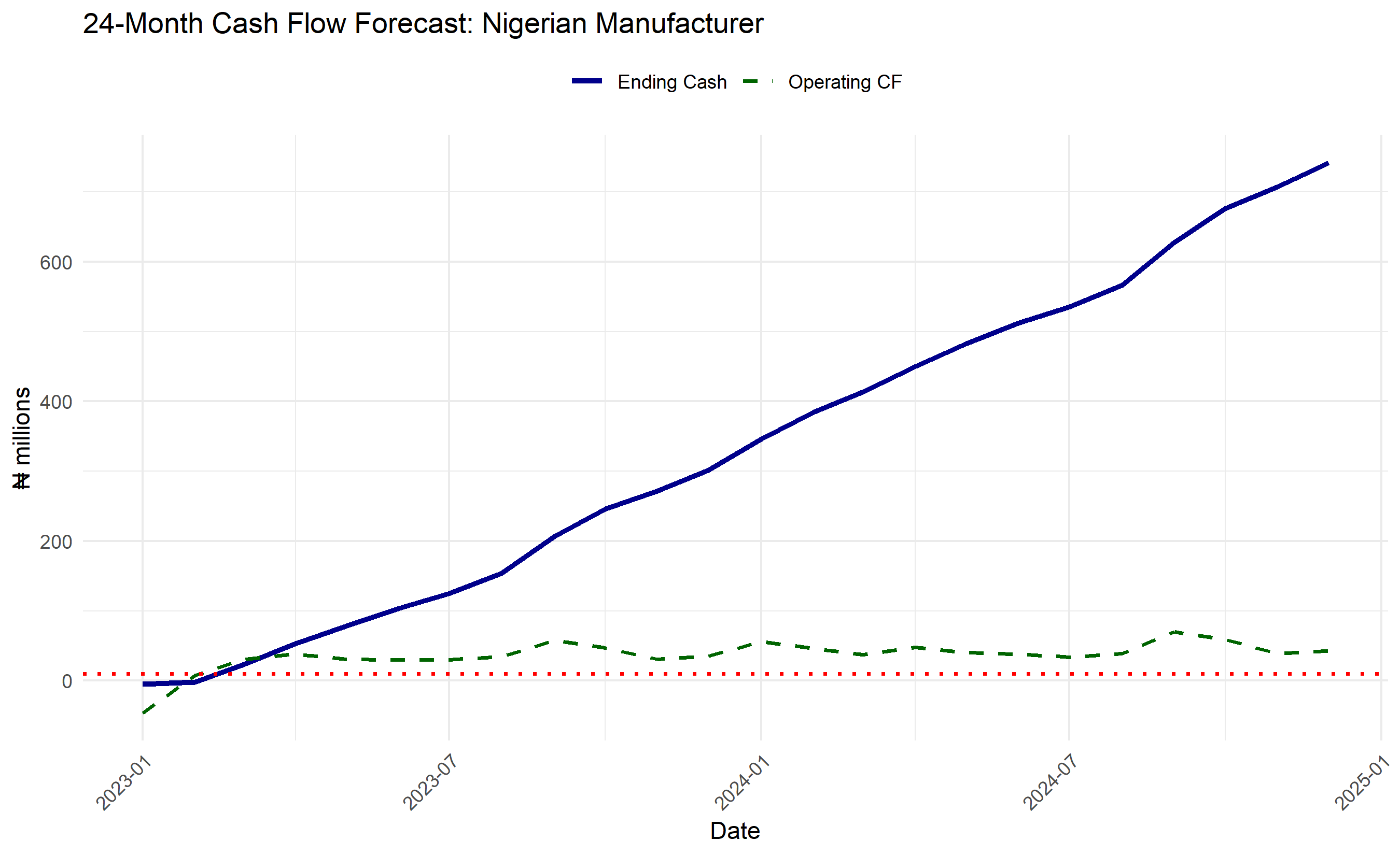
📝 Section 26.6 Review Questions

In the Monte Carlo output, if the 5th percentile is ₦5M and the mean is ₦40M, what does this asymmetry suggest?
If 15% of simulations show negative cash, what actions should the CFO take?
How would you use the 95th percentile (upside) forecast to decide on dividend policy?
Compare the Monte Carlo approach to deterministic scenario analysis. What insights does Monte Carlo add?
If the probability of cash shortfall is 2%, do you still need a credit line? Why or why not?

31.7 Chapter Exercises

Chapter 26 Exercises

Exercise 26.1: Reading and Interpreting a Cash Flow Statement

A Nigerian retail company provides the following summary cash flow data for the last quarter:

Item	Amount (₦ millions)
Net profit after tax	45.0
Add: Depreciation	8.5
(Decrease)/Increase in trade receivables	(12.0)
(Decrease)/Increase in inventory	(18.5)
Increase/(Decrease) in trade payables	7.0
Operating Cash Flow	?
Capital expenditure on new equipment	(25.0)
Proceeds from sale of old machinery	4.0
Investing Cash Flow	?
New bank loan received	30.0
Loan repayment	(15.0)
Dividend paid	(10.0)
Financing Cash Flow	?
Net Change in Cash	?
Opening cash balance	22.5
Closing cash balance	?

Complete the table: calculate Operating Cash Flow, Investing Cash Flow, Financing Cash Flow, Net Change in Cash, and the Closing Cash Balance.
Despite a net profit of ₦45 million, the company’s operating cash flow is much lower. Explain why this can happen, using the specific items in the table above.
The company borrowed ₦30 million and spent ₦25 million on equipment. How would you interpret this combination of investing and financing activities? Is this a sign of financial strength or stress?
A bank is considering giving this company a short-term working capital loan. Using only the information in this cash flow statement, identify two things that would concern you and one thing that would be reassuring.

Exercise 26.2: The Cash Conversion Cycle

A manufacturing company in Aba has the following data: - Annual credit sales: ₦720 million - Cost of goods sold: ₦480 million
- Average accounts receivable: ₦120 million - Average inventory: ₦80 million - Average accounts payable: ₦60 million

Calculate the Days Sales Outstanding (DSO): Average Receivables ÷ (Annual Sales ÷ 365)
Calculate the Days Inventory Outstanding (DIO): Average Inventory ÷ (COGS ÷ 365)
Calculate the Days Payable Outstanding (DPO): Average Payables ÷ (COGS ÷ 365)
Calculate the Cash Conversion Cycle (CCC): DSO + DIO − DPO
The industry average CCC is 45 days. How does this company compare? What specific action would reduce the CCC by the greatest amount?
If the company could reduce DSO by 10 days (collecting receivables faster), how much cash would this release, assuming the same annual sales level? Show your calculation.

Exercise 26.3: Building a 13-Week Cash Flow Forecast

You are the CFO of a trading company in Lagos. You need to build a 13-week direct cash flow forecast. From your records and business plans, you know:

Inflows: - Collections from customers (credit sales from prior weeks, typically 60% collected in 2 weeks, 30% in 4 weeks, 10% in 6 weeks) - This week’s credit sales: ₦8 million; growing at 5% per week for the first month, then flat

Outflows: - Supplier payments: ₦4 million per week (due 3 weeks after purchase) - Wages: ₦1.5 million every 2 weeks (next payroll in Week 2) - Rent: ₦0.8 million in Week 4 and Week 13 - Tax instalment: ₦2.0 million in Week 8

Opening cash balance: ₦6 million

For each of the first 6 weeks, calculate total cash inflows from collections (using the collection pattern above). Show how collections in Week 3, for example, depend on sales from Weeks 1 and 2.
List all cash outflows for each of the 13 weeks.
Calculate the net cash flow and running cash balance week by week.
In which week(s), if any, does the cash balance fall below ₦2 million (your minimum operating buffer)? What would you do in advance of this point?
Identify the peak cash deficit period. If you needed to arrange a revolving credit facility, what size would you request from your bank, and when would you need it in place?

Exercise 26.4: Stress Testing a Cash Flow Forecast

Using the forecast from Exercise 26.3 (or your own version), build a simple stress test.

Scenario 1 (Slow collections): Suppose customers pay more slowly — only 40% collected in 2 weeks, 40% in 4 weeks, 20% in 6 weeks. Recalculate the 13-week cash flow and identify the worst week.
Scenario 2 (Revenue shock): In Week 5, a major customer cancels their order, reducing weekly sales by ₦3 million for 4 weeks. Recalculate.
Scenario 3 (Combined): Apply both slow collections AND the revenue shock simultaneously. What is the worst-case ending cash balance?
Create a simple summary table showing the ending cash balance under Base Case, Scenario 1, Scenario 2, and Scenario 3. Present this in a format suitable for a board meeting.
What specific management actions could the company take in advance to protect against each scenario? Suggest at least two practical actions per scenario.

Exercise 26.5: Machine Learning vs. Traditional Forecasting for Cash Flows

A large telecoms company has 5 years of daily cash inflow and outflow data. Their Treasury team uses a traditional 13-week rolling forecast built in Excel. A data scientist proposes replacing this with an XGBoost model trained on the historical data.

List three advantages of using a machine learning model for cash flow forecasting over a traditional spreadsheet-based approach.
List three challenges or risks of the machine learning approach that the Excel approach does not have.
The Finance Director asks: “If the model was trained on normal operating periods, what happens if there’s a financial crisis or a major regulatory change?” How would you address this concern?
Propose a hybrid approach that combines the strengths of both methods. Describe in 3–4 sentences how this would work in practice.
How would you evaluate the performance of the cash flow forecasting model over time? Describe the specific metrics and monitoring process you would put in place.

31.8 Further Reading

Damodaran, A. (2012). Corporate Finance: Theory and Practice (3rd ed.). John Wiley & Sons. Chapter on working capital and cash flow forecasting.
Vélez-Pareja, I., & Burbano-Pérez, A. (2005). Evaluating working capital management through cash conversion cycle: A case study in Latin America. Journal of Applied Finance, 15(2), 60–72.
Shim, J. K., & Siegel, J. G. (2012). Handbook of Financial Analysis, Forecasting, and Modeling (3rd ed.). Business Expert Press. Chapters on cash flow and scenario analysis.
Wilmott, P. (2019). Machine Learning in Finance: The Case for a Bayesian Approach. Wiley. Section on quantile forecasting for financial risk.

31.9 Chapter 26 Appendix: Mathematical Derivations

31.9.1 A26.1 Pinball (Quantile) Loss Function Derivation

The pinball loss for quantile \(\tau\) is defined as: \[L_\tau(y, \hat{y}) = \begin{cases} \tau(y - \hat{y}) & \text{if } y > \hat{y} \\ (\tau - 1)(y - \hat{y}) & \text{if } y \leq \hat{y} \end{cases}\]

This can be written compactly as: \[L_\tau(y, \hat{y}) = (\tau - \mathbb{1}_{y < \hat{y}}) (y - \hat{y}) = (\tau - \mathbb{1}_{\epsilon < 0}) \epsilon\] where \(\epsilon = y - \hat{y}\) is the error and \(\mathbb{1}_{\cdot}\) is the indicator function.

Intuition: For an over-prediction (\(y < \hat{y}\), so \(\epsilon < 0\)), the loss is \((\tau - 1) |\epsilon|\). Since \(\tau - 1 < 0\), the coefficient is negative, but we typically report the absolute value. The loss is proportional to \((1 - \tau)\). For \(\tau = 0.9\) (90th percentile), the coefficient is \((1 - 0.9) = 0.1\), penalising over-predictions lightly. For an under-prediction (\(y > \hat{y}\), so \(\epsilon > 0\)), the loss is \(\tau |\epsilon|\). For \(\tau = 0.9\), the coefficient is 0.9, penalising under-predictions heavily.

Minimisation: To estimate the conditional \(\tau\)-quantile, fit a linear model \(\hat{y} = X\beta\) by minimising: \[\min_\beta \sum_{i=1}^{n} L_\tau(y_i, X_i \beta)\]

This is a linear programming problem, solved by QR (quantile regression) algorithms.

31.9.2 A26.2 Quantile Regression as Linear Programming

The quantile regression problem: \[\min_\beta \sum_{i=1}^{n} L_\tau(y_i, X_i \beta)\]

can be reformulated as: \[\min_{\beta, u, v} \sum_{i=1}^{n} (\tau u_i + (1 - \tau) v_i)\] subject to: \[y_i - X_i \beta = u_i - v_i, \quad u_i, v_i \geq 0\]

Here \(u_i\) and \(v_i\) are positive and negative residuals, respectively. The objective weights positive residuals by \(\tau\) and negative residuals by \((1 - \tau)\). This is a linear program (LP) and can be solved efficiently using interior-point or simplex methods.

31.9.3 A26.3 Cash Conversion Cycle: Working Capital Finance

The Cash Conversion Cycle (CCC) measures the days between cash outflow for inventory and cash inflow from sales: \[\text{CCC} = \text{DIO} + \text{DSO} - \text{DPO}\]

Interpretation: - DIO (Days Inventory Outstanding): Days inventory is held. Reducing DIO (faster turnover) frees cash. - DSO (Days Sales Outstanding): Days to collect from customers. Reducing DSO (faster payment terms) frees cash. - DPO (Days Payable Outstanding): Days to pay suppliers. Increasing DPO (negotiating longer terms) delays outflow, freeing cash.

Example: A firm with DIO = 30, DSO = 60, DPO = 30 has: \[\text{CCC} = 30 + 60 - 30 = 60 \text{ days}\]

Financially, the firm must finance 60 days of operations. If daily operating costs are ₦500,000, the firm needs ₦30M in working capital.

Optimisation: A firm can reduce CCC by: 1. Reducing DIO (just-in-time inventory, better demand forecasting). 2. Reducing DSO (tighter credit policies, early payment discounts, factor receivables). 3. Increasing DPO (negotiate longer payment terms, but maintain supplier relationships).

A 10-day reduction in CCC frees ₦5M in the example above.

31.9.4 A26.4 Monte Carlo Value-at-Risk Estimation

From a Monte Carlo sample \(\{C^{(1)}, C^{(2)}, \ldots, C^{(N)}\}\) of ending cash balances:

Empirical Quantile (nonparametric VaR): \[\text{VaR}_\alpha = C_{(\lceil (1 - \alpha) N \rceil)}\] where \(C_{(k)}\) is the \(k\)-th order statistic (sorted value) and \(\alpha\) is the confidence level. For \(\alpha = 0.05\) (95% confidence, 5% tail), we report the 5th percentile (0.05 × 1000 = 50th smallest value).

Expected Shortfall (tail risk beyond VaR): \[\text{ES}_\alpha = \mathbb{E}[C | C \leq \text{VaR}_\alpha] \approx \frac{1}{\lceil \alpha N \rceil} \sum_{i=1}^{\lceil \alpha N \rceil} C_{(i)}\]

This is the average of all outcomes worse than VaR, providing the expected loss if the worst case occurs.

Practical Use: If VaR₀.₀₅ = ₦10M and ES₀.₀₅ = ₦5M, there’s a 5% chance cash falls below ₦10M, and conditional on that, the average balance is ₦5M (deeply negative). The CFO should plan for this tail risk, e.g., by arranging a ₦15M credit line.