---
title: "Classical Forecasting: ARIMA and Exponential Smoothing"
author: "Bongo Adi"
date: "2024"
number-sections: true
---
```{python}
#| label: python-setup-24-arima-exponential-smoothing
#| include: false
import numpy as np
import pandas as pd
import matplotlib.pyplot as plt
import seaborn as sns
from statsmodels.tsa.holtwinters import SimpleExpSmoothing, ExponentialSmoothing
from datetime import datetime, timedelta
from statsmodels.tsa.holtwinters import ExponentialSmoothing
from statsmodels.tsa.arima.model import ARIMA
from statsmodels.graphics.tsaplots import plot_acf, plot_pacf
from statsmodels.stats.diagnostic import acorr_ljungbox
from scipy import stats
from statsmodels.tsa.statespace.sarimax import SARIMAX
```
::: {.callout-note icon="false"}
## 📋 Learning Objectives
By the end of this chapter, you will:
- Understand exponential smoothing as a recursive forecasting framework (SES, Holt, Holt-Winters)
- Implement ARIMA(p,d,q) models: identify orders using ACF/PACF, fit via MLE, diagnose residuals
- Choose between seasonal (SARIMA) and non-seasonal ARIMA using information criteria
- Apply auto.arima to automate parameter selection
- Quantify forecast uncertainty via prediction intervals
- Communicate forecasts and uncertainty to non-technical stakeholders
- Build production-ready forecasts for Nigerian FX rates and economic metrics
:::
## Simple Exponential Smoothing (SES): The Forgetting Principle
Exponential smoothing is an elegant recursive framework for forecasting. The core idea: **recent observations are more informative than distant ones**, so weight them more heavily. But rather than explicitly choosing weights (difficult!), use a single smoothing parameter $\alpha$ to control decay.
### The SES Recursion
Simple exponential smoothing for a series without trend or seasonality:
$$\hat{Y}_{t+1} = \alpha Y_t + (1 - \alpha) \hat{Y}_{t}$$
where $\hat{Y}_{t+1}$ is the forecast for time $t+1$ given data through time $t$, and $\alpha \in [0, 1]$ is the smoothing parameter.
**Intuition**: The forecast is a weighted average of the current observation ($Y_t$, weight $\alpha$) and the prior forecast ($\hat{Y}_t$, weight $1 - \alpha$).
- If $\alpha$ is close to 1, we trust recent data heavily (forecast reacts quickly to changes).
- If $\alpha$ is close to 0, we update slowly (forecast is more stable, less reactive).
### Equivalently: SES as an Infinite Moving Average
Expanding the recursion:
$$\hat{Y}_{t+1} = \alpha Y_t + (1 - \alpha) \hat{Y}_t = \alpha Y_t + (1 - \alpha) [\alpha Y_{t-1} + (1 - \alpha) \hat{Y}_{t-1}]$$
$$= \alpha Y_t + \alpha(1 - \alpha) Y_{t-1} + \alpha(1 - \alpha)^2 Y_{t-2} + \cdots$$
So the forecast is a weighted average of all past observations, with exponentially decaying weights. Distant observations have negligible influence.
### Fitting SES: Choosing the Optimal $\alpha$
In practice, $\alpha$ is chosen by minimising the sum of squared one-step-ahead forecast errors (SSE):
$$\text{SSE} = \sum_{t=2}^{T} (Y_t - \hat{Y}_t)^2$$
This is done via numerical optimisation. Most software (R, Python) defaults provide good $\alpha$ estimates.
### Applying SES to Nigerian Petrol Price
::: {.panel-tabset}
## R
```{r}
library(forecast)
library(tidyverse)
# Generate synthetic Nigerian petrol price data (monthly, 2015-2023)
set.seed(42)
n_months_petrol <- 108
dates_petrol <- seq(from = ymd("2015-01-01"), by = "month", length.out = n_months_petrol)
# Petrol price: upward trend with some noise
base_price <- 50
trend_petrol <- base_price + 0.1 * (1:n_months_petrol) + 10 * sin(2 * pi * (1:n_months_petrol) / 24)
noise_petrol <- rnorm(n_months_petrol, 0, 2)
petrol_price <- trend_petrol + noise_petrol
petrol_ts <- ts(petrol_price, start = c(2015, 1), frequency = 12)
# Fit SES with optimal alpha
ses_fit <- ses(petrol_ts, alpha = NULL, initial = "optimal", h = 12)
cat("=== Simple Exponential Smoothing (SES) ===\n")
cat("Optimal smoothing parameter (alpha):", round(ses_fit$model$par['alpha'], 3), "\n")
cat("AIC:", round(ses_fit$model$aic, 1), "\n\n")
# Forecast next 12 months
forecast_ses <- forecast(ses_fit, h = 12)
# Plot
autoplot(petrol_ts) +
autolayer(forecast_ses, alpha = 0.7, PI = TRUE) +
theme_minimal() +
labs(title = "Nigerian Petrol Price: SES Forecast",
x = "Date", y = "Price (NGN/litre)") +
theme(legend.position = "bottom")
# Print forecast
cat("=== SES Forecast (next 12 months) ===\n")
print(forecast_ses)
```
## Python
```{python}
from statsmodels.tsa.holtwinters import SimpleExpSmoothing, ExponentialSmoothing
import pandas as pd
import numpy as np
import matplotlib.pyplot as plt
from datetime import datetime, timedelta
# Generate synthetic Nigerian petrol price
np.random.seed(42)
n_months_petrol = 108
dates_petrol = pd.date_range(start='2015-01-01', periods=n_months_petrol, freq='MS')
base_price = 50
trend_petrol = base_price + 0.1 * np.arange(1, n_months_petrol + 1) + 10 * np.sin(2 * np.pi * np.arange(1, n_months_petrol + 1) / 24)
noise_petrol = np.random.normal(0, 2, n_months_petrol)
petrol_price = trend_petrol + noise_petrol
petrol_ts = pd.Series(petrol_price, index=dates_petrol)
# Fit SES
ses_model = SimpleExpSmoothing(petrol_ts)
ses_fit = ses_model.fit(optimized=True)
print("=== Simple Exponential Smoothing (SES) ===")
print(f"Optimal smoothing parameter (alpha): {ses_fit.params['smoothing_level']:.3f}")
print(f"AIC: {ses_fit.aic:.1f}\n")
# Forecast (SimpleExpSmoothing uses .forecast(), not .get_forecast())
n_forecast = 12
forecast_values = ses_fit.forecast(steps=n_forecast)
forecast_dates = pd.date_range(start=petrol_ts.index[-1] + pd.DateOffset(months=1),
periods=n_forecast, freq='MS')
forecast_mean = pd.Series(forecast_values.values, index=forecast_dates)
# Approximate 95% CI from in-sample residuals
sigma = ses_fit.resid.std()
lower_ci = forecast_mean - 1.96 * sigma
upper_ci = forecast_mean + 1.96 * sigma
# Plot
fig, ax = plt.subplots(figsize=(12, 6))
ax.plot(petrol_ts.index, petrol_ts.values, color='black', linewidth=1.5, label='Historical Data')
ax.plot(forecast_mean.index, forecast_mean.values, color='blue', linewidth=2, label='SES Forecast')
ax.fill_between(forecast_mean.index, lower_ci, upper_ci,
alpha=0.2, color='blue', label='95% Prediction Interval')
ax.set_title('Nigerian Petrol Price: SES Forecast', fontsize=12, fontweight='bold')
ax.set_xlabel('Date')
ax.set_ylabel('Price (NGN/litre)')
ax.legend()
ax.grid(True, alpha=0.3)
plt.tight_layout()
plt.savefig('ses_forecast.png', dpi=150, bbox_inches='tight')
print("Plot saved as 'ses_forecast.png'")
# Print forecast
print("\n=== SES Forecast (next 12 months) ===")
forecast_df = pd.DataFrame({
'Forecast': forecast_mean.values,
'Lower_CI': lower_ci.values,
'Upper_CI': upper_ci.values
}, index=forecast_mean.index)
print(forecast_df.round(2))
```
:::
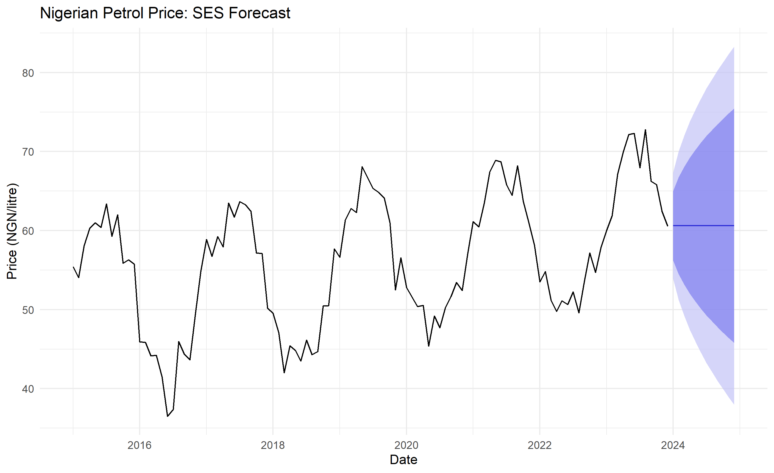
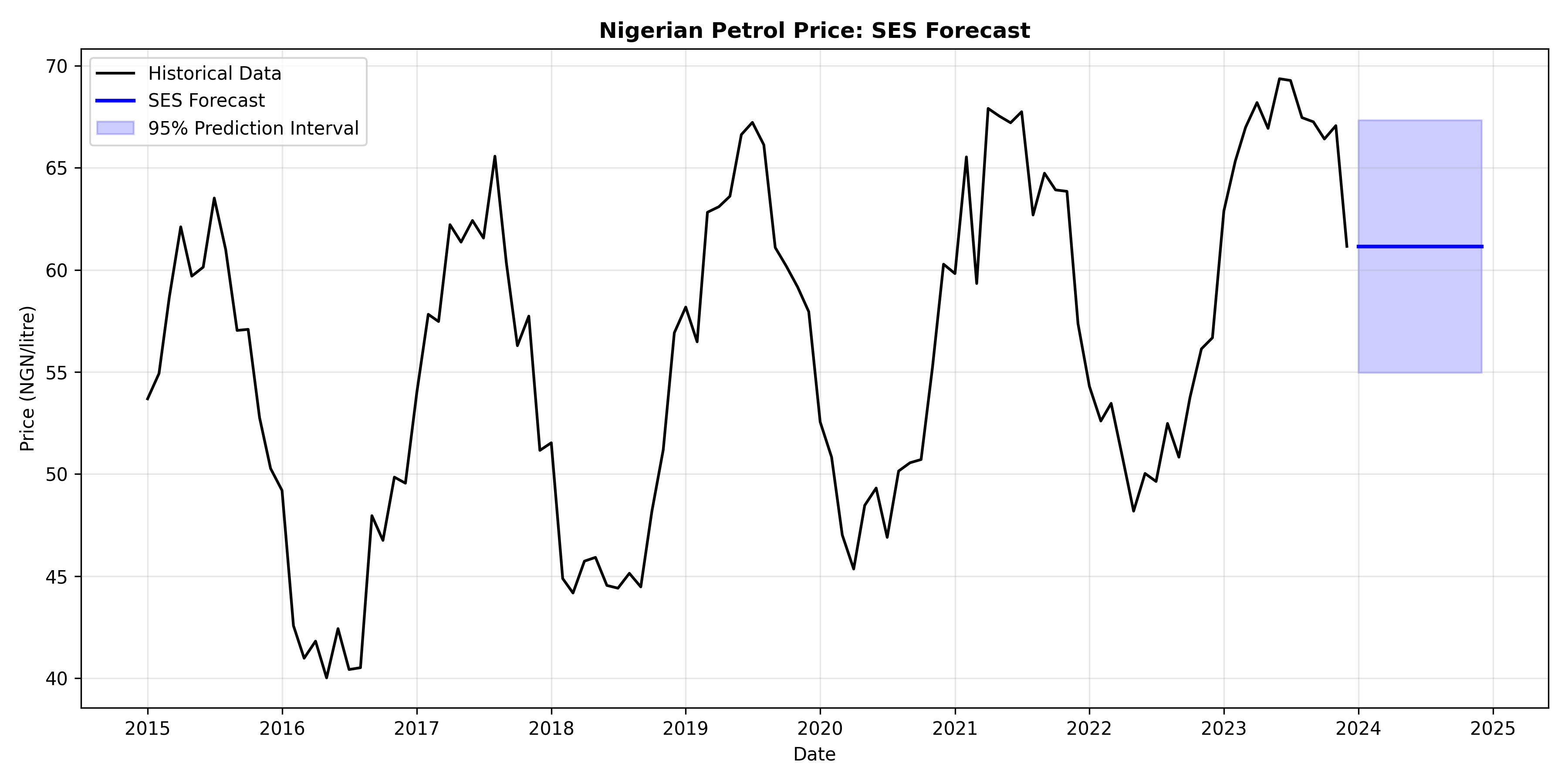
SES automatically chooses $\alpha$ to minimise forecast error, then projects forward. The forecast is flat (constant) because SES assumes no trend or seasonality—a reasonable assumption for many stationary series but crude for trending data.
::: {.callout-caution icon="false"}
## 📝 Section 24.1 Review Questions
1. If $\alpha = 0.9$, does the forecast adapt quickly or slowly to new data?
2. SES forecast is always a constant (horizontal line into the future). Is this a strength or weakness?
3. How would you choose between $\alpha = 0.2$ and $\alpha = 0.8$ without fitting both? (Hint: look at the data visually.)
4. What is the initial condition $\hat{Y}_1$? How does it affect the forecast?
:::
## Holt's Linear Trend Method
If data exhibits a trend, SES is inappropriate. Holt's method extends SES with a **level** and **trend** component:
$$\ell_t = \alpha Y_t + (1 - \alpha)(\ell_{t-1} + b_{t-1})$$
$$b_t = \beta (\ell_t - \ell_{t-1}) + (1 - \beta) b_{t-1}$$
$$\hat{Y}_{t+h} = \ell_t + h \cdot b_t$$
where $\ell_t$ is the estimated level (baseline), $b_t$ is the estimated trend (slope), $\alpha$ controls level smoothing, and $\beta$ controls trend smoothing.
The forecast is a linear extrapolation: current level plus $h$ periods of the current trend.
### Fitting Holt's Method
Similar to SES, $\alpha$ and $\beta$ are chosen to minimise forecast errors. Most software provides automatic selection.
::: {.panel-tabset}
## R
```{r}
# Fit Holt's linear trend method to petrol price
holt_fit <- holt(petrol_ts, alpha = NULL, beta = NULL, initial = "optimal", h = 12)
cat("=== Holt's Linear Trend Method ===\n")
cat("Smoothing parameter (alpha):", round(holt_fit$model$par['alpha'], 3), "\n")
cat("Trend parameter (beta):", round(holt_fit$model$par['beta'], 3), "\n")
cat("AIC:", round(holt_fit$model$aic, 1), "\n\n")
# Forecast
forecast_holt <- forecast(holt_fit, h = 12)
# Plot
autoplot(petrol_ts) +
autolayer(forecast_holt, alpha = 0.7, PI = TRUE) +
theme_minimal() +
labs(title = "Nigerian Petrol Price: Holt's Linear Trend Forecast",
x = "Date", y = "Price (NGN/litre)") +
theme(legend.position = "bottom")
# Compare SES vs Holt
cat("=== SES vs. Holt Comparison ===\n")
cat("SES AIC:", round(ses_fit$model$aic, 1), "\n")
cat("Holt AIC:", round(holt_fit$model$aic, 1), "\n")
cat("Better: ", ifelse(holt_fit$model$aic < ses_fit$model$aic, "Holt", "SES"), "\n")
```
## Python
```{python}
from statsmodels.tsa.holtwinters import ExponentialSmoothing
# Fit Holt's linear trend method
holt_model = ExponentialSmoothing(petrol_ts, trend='add', seasonal=None, initialization_method='estimated')
holt_fit = holt_model.fit(optimized=True)
print("=== Holt's Linear Trend Method ===")
print(f"Smoothing parameter (alpha): {holt_fit.params['smoothing_level']:.3f}")
print(f"Trend parameter (beta): {holt_fit.params['smoothing_trend']:.3f}")
print(f"AIC: {holt_fit.aic:.1f}\n")
# Forecast (ExponentialSmoothing uses .forecast(), not .get_forecast())
n_steps_holt = 12
forecast_holt_values = holt_fit.forecast(steps=n_steps_holt)
forecast_holt_dates = pd.date_range(start=petrol_ts.index[-1] + pd.DateOffset(months=1),
periods=n_steps_holt, freq='MS')
forecast_holt_mean = pd.Series(forecast_holt_values.values, index=forecast_holt_dates)
sigma_holt = holt_fit.resid.std()
holt_lower = forecast_holt_mean - 1.96 * sigma_holt
holt_upper = forecast_holt_mean + 1.96 * sigma_holt
# Plot
fig, ax = plt.subplots(figsize=(12, 6))
ax.plot(petrol_ts.index, petrol_ts.values, color='black', linewidth=1.5, label='Historical Data')
ax.plot(forecast_holt_mean.index, forecast_holt_mean.values, color='darkgreen', linewidth=2, label="Holt's Trend Forecast")
ax.fill_between(forecast_holt_mean.index, holt_lower, holt_upper,
alpha=0.2, color='darkgreen', label='95% Prediction Interval')
ax.set_title("Nigerian Petrol Price: Holt's Linear Trend Forecast", fontsize=12, fontweight='bold')
ax.set_xlabel('Date')
ax.set_ylabel('Price (NGN/litre)')
ax.legend()
ax.grid(True, alpha=0.3)
plt.tight_layout()
plt.savefig('holt_forecast.png', dpi=150, bbox_inches='tight')
print("Plot saved as 'holt_forecast.png'")
# Compare
print("\n=== SES vs. Holt Comparison ===")
ses_aic = ses_fit.aic
holt_aic = holt_fit.aic
print(f"SES AIC: {ses_aic:.1f}")
print(f"Holt AIC: {holt_aic:.1f}")
print(f"Better: {'Holt' if holt_aic < ses_aic else 'SES'}")
```
:::
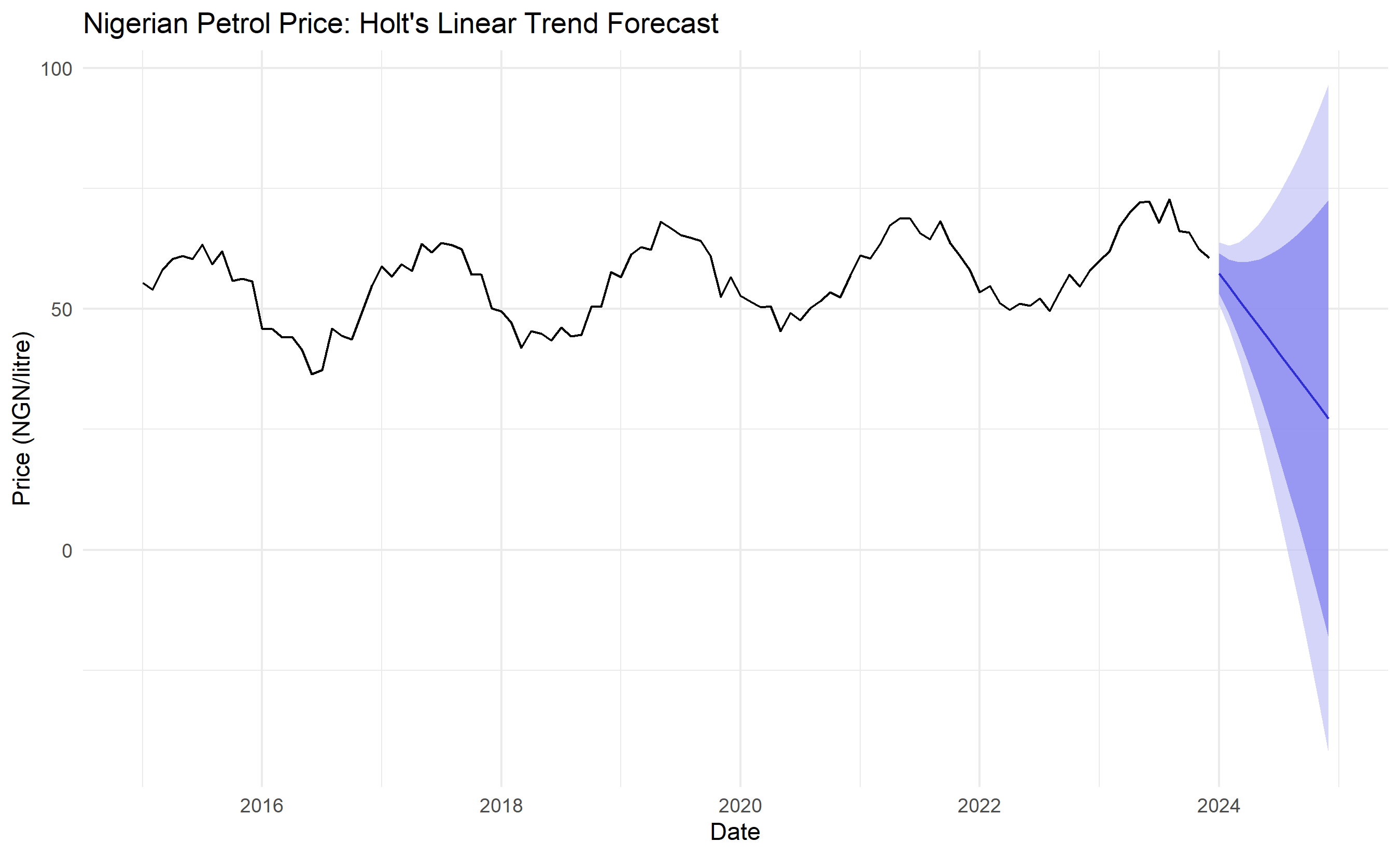
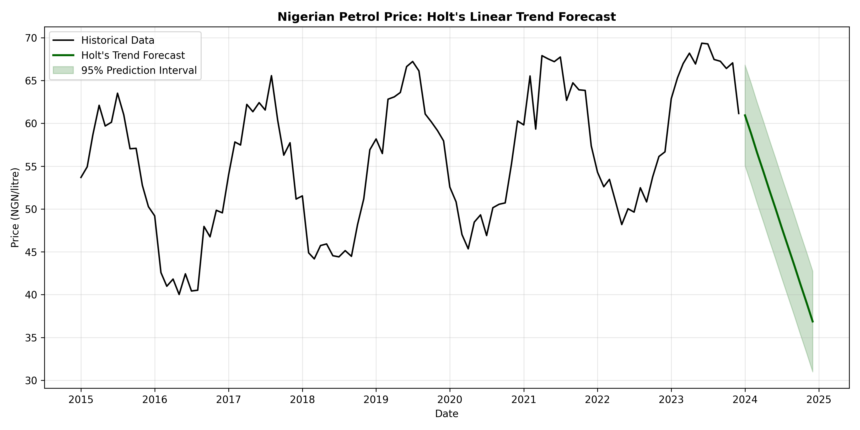
Holt's method produces a sloped forecast line, capturing the trend. The forecast continues linearly into the future. This is more realistic for trending data than SES's flat forecast.
::: {.callout-caution icon="false"}
## 📝 Section 24.2 Review Questions
1. Holt's forecast continues linearly forever. Is this realistic for petrol prices? What could go wrong?
2. What is the relationship between $\beta$ (trend smoothing) and trend persistence? If $\beta = 0$, what happens?
3. How would you modify Holt's method to forecast a trend that is decelerating (getting flatter over time)?
:::
## Holt-Winters Seasonal Method
The final extension adds **seasonality** via Holt-Winters:
$$\ell_t = \alpha \frac{Y_t}{s_{t-m}} + (1 - \alpha)(\ell_{t-1} + b_{t-1})$$
$$b_t = \beta (\ell_t - \ell_{t-1}) + (1 - \beta) b_{t-1}$$
$$s_t = \gamma \frac{Y_t}{\ell_t} + (1 - \gamma) s_{t-m}$$
$$\hat{Y}_{t+h} = (\ell_t + h \cdot b_t) \cdot s_{t+h-m}$$
(This is the multiplicative version; an additive version exists for series without proportional seasonality.)
**Three smoothing parameters**:
- $\alpha$: level smoothing.
- $\beta$: trend smoothing.
- $\gamma$: seasonal smoothing.
The seasonal indices $s_t$ are stored and recycled. If $m = 12$ (monthly), the seasonal factor repeats every 12 months.
### Applying Holt-Winters to Nigerian Retail Revenue
::: {.panel-tabset}
## R
```{r}
# Generate synthetic Nigerian retail revenue (monthly, strong seasonality)
set.seed(42)
n_months_retail <- 120
dates_retail <- seq(from = ymd("2014-01-01"), by = "month", length.out = n_months_retail)
# Retail revenue: upward trend + strong seasonality (December peak)
base_revenue <- 1000
trend_retail <- base_revenue + 1.5 * (1:n_months_retail)
seasonality_retail <- 200 * sin(2 * pi * (1:n_months_retail) / 12 - pi/2) +
150 * sin(2 * pi * (1:n_months_retail) / 6) # Semi-annual
noise_retail <- rnorm(n_months_retail, 0, 50)
revenue <- trend_retail + seasonality_retail + noise_retail
revenue_ts <- ts(revenue, start = c(2014, 1), frequency = 12)
# Fit Holt-Winters (multiplicative for growing seasonality)
hw_fit <- hw(revenue_ts, seasonal = "mult", h = 24)
cat("=== Holt-Winters Seasonal Method ===\n")
cat("Smoothing parameters:\n")
cat(" Alpha (level):", round(hw_fit$model$par['alpha'], 3), "\n")
cat(" Beta (trend):", round(hw_fit$model$par['beta'], 3), "\n")
cat(" Gamma (seasonal):", round(hw_fit$model$par['gamma'], 3), "\n")
cat("AIC:", round(hw_fit$model$aic, 1), "\n\n")
# Forecast 24 months ahead
forecast_hw <- forecast(hw_fit, h = 24)
# Plot
autoplot(revenue_ts) +
autolayer(forecast_hw, alpha = 0.7, PI = TRUE) +
theme_minimal() +
labs(title = "Nigerian Retail Revenue: Holt-Winters Seasonal Forecast",
x = "Date", y = "Revenue (NGN millions)") +
theme(legend.position = "bottom")
print(forecast_hw)
```
## Python
```{python}
# Generate synthetic Nigerian retail revenue
np.random.seed(42)
n_months_retail = 120
dates_retail = pd.date_range(start='2014-01-01', periods=n_months_retail, freq='MS')
base_revenue = 1000
trend_retail = base_revenue + 1.5 * np.arange(1, n_months_retail + 1)
seasonality_retail = (200 * np.sin(2 * np.pi * np.arange(1, n_months_retail + 1) / 12 - np.pi/2) +
150 * np.sin(2 * np.pi * np.arange(1, n_months_retail + 1) / 6))
noise_retail = np.random.normal(0, 50, n_months_retail)
revenue = trend_retail + seasonality_retail + noise_retail
revenue_ts = pd.Series(revenue, index=dates_retail)
# Fit Holt-Winters (multiplicative)
hw_model = ExponentialSmoothing(revenue_ts, trend='add', seasonal='mul', seasonal_periods=12, initialization_method='estimated')
hw_fit = hw_model.fit(optimized=True)
print("=== Holt-Winters Seasonal Method ===")
print(f"Smoothing parameters:")
print(f" Alpha (level): {hw_fit.params['smoothing_level']:.3f}")
print(f" Beta (trend): {hw_fit.params['smoothing_trend']:.3f}")
print(f" Gamma (seasonal): {hw_fit.params['smoothing_seasonal']:.3f}")
print(f"AIC: {hw_fit.aic:.1f}\n")
# Forecast 24 months (ExponentialSmoothing uses .forecast(), not .get_forecast())
n_steps_hw = 24
forecast_hw_values = hw_fit.forecast(steps=n_steps_hw)
forecast_hw_dates = pd.date_range(start=revenue_ts.index[-1] + pd.DateOffset(months=1),
periods=n_steps_hw, freq='MS')
forecast_hw_mean = pd.Series(forecast_hw_values.values, index=forecast_hw_dates)
sigma_hw = hw_fit.resid.std()
hw_lower = forecast_hw_mean - 1.96 * sigma_hw
hw_upper = forecast_hw_mean + 1.96 * sigma_hw
# Plot
fig, ax = plt.subplots(figsize=(12, 6))
ax.plot(revenue_ts.index, revenue_ts.values, color='black', linewidth=1.5, label='Historical Data')
ax.plot(forecast_hw_mean.index, forecast_hw_mean.values, color='purple', linewidth=2, label='Holt-Winters Forecast')
ax.fill_between(forecast_hw_mean.index, hw_lower, hw_upper,
alpha=0.2, color='purple', label='95% Prediction Interval')
ax.set_title('Nigerian Retail Revenue: Holt-Winters Seasonal Forecast', fontsize=12, fontweight='bold')
ax.set_xlabel('Date')
ax.set_ylabel('Revenue (NGN millions)')
ax.legend()
ax.grid(True, alpha=0.3)
plt.tight_layout()
plt.savefig('hw_forecast.png', dpi=150, bbox_inches='tight')
print("Plot saved as 'hw_forecast.png'")
print("\n=== Holt-Winters Forecast (next 24 months, first 12 shown) ===")
print(forecast_hw_mean.head(12).round(1))
```
:::
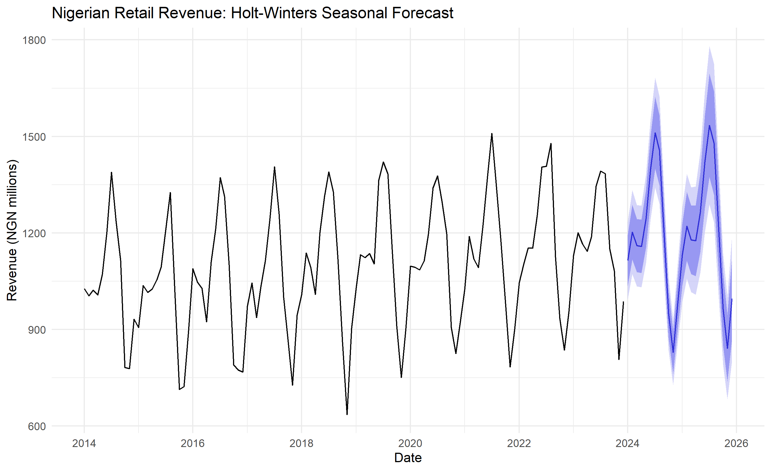
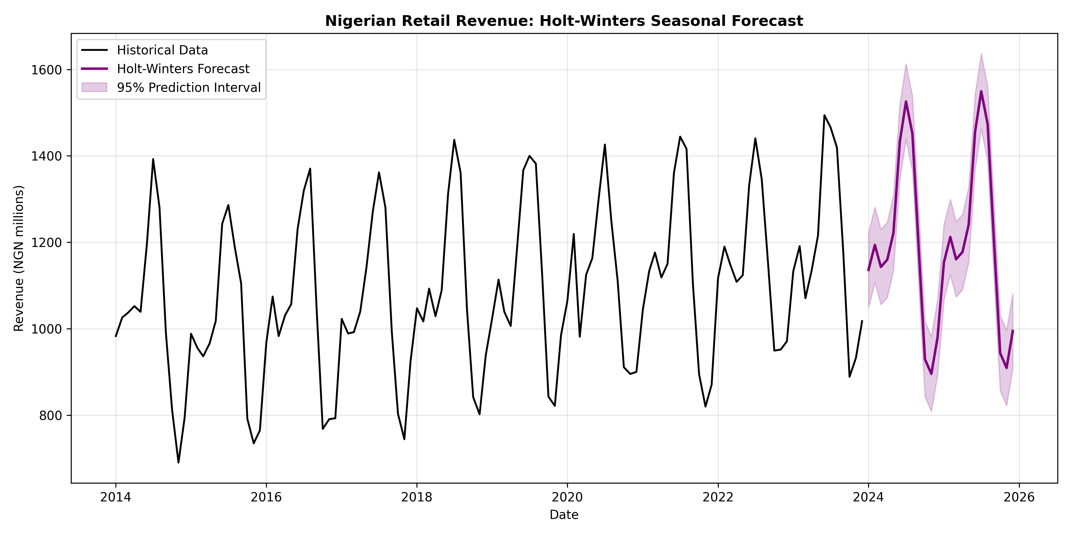
Holt-Winters captures both the upward trend and the seasonal pattern, producing a forecast that rises over time while oscillating with the seasonal cycle. This is much more realistic for retail or other seasonal businesses.
::: {.callout-caution icon="false"}
## 📝 Section 24.3 Review Questions
1. When would you use additive seasonality vs. multiplicative seasonality?
2. Holt-Winters has three parameters ($\alpha, \beta, \gamma$). Are they always all estimated? What if the data has no trend?
3. If you forecast 24 months and the seasonal pattern repeats every 12 months, will the forecast eventually converge to the trend line?
:::
## The ARIMA Model Family: AR, MA, I, and Combinations
ARIMA (AutoRegressive Integrated Moving Average) is a powerful framework unifying three concepts:
**AR(p): Autoregressive**
The observation is a linear combination of its past values:
$$Y_t = c + \phi_1 Y_{t-1} + \phi_2 Y_{t-2} + \cdots + \phi_p Y_{t-p} + \epsilon_t$$
The series "remembers" its past. An AR(1) process with $\phi_1 = 0.7$ means today's value is 70% of yesterday plus noise.
**MA(q): Moving Average**
The observation is a linear combination of past shocks (forecast errors):
$$Y_t = \mu + \epsilon_t + \theta_1 \epsilon_{t-1} + \theta_2 \epsilon_{t-2} + \cdots + \theta_q \epsilon_{t-q}$$
Current value depends on recent noise terms, not on past Y values directly.
**I(d): Integrated (differenced)**
Take the original series and difference it $d$ times to achieve stationarity:
$$\Delta^d Y_t$$
$d = 0$ means no differencing (series is already stationary). $d = 1$ means first differences (common for trending data).
**ARIMA(p, d, q)**: Combine all three.
Fit an AR(p) model to the $d$-times-differenced series, with an MA(q) error term.
### Example: ARIMA(1, 1, 1)
$$\Delta Y_t = c + \phi_1 \Delta Y_{t-1} + \epsilon_t + \theta_1 \epsilon_{t-1}$$
First difference the original series, then fit an ARMA(1, 1) model (AR with MA errors).
::: {.callout-caution icon="false"}
## 📝 Section 24.4 Review Questions
1. If a series is non-stationary, should you set $d = 0$ or $d > 0$? Why?
2. An AR(1) with $\phi_1 = 0.95$ vs. $\phi_1 = 0.5$: which has more persistence? Which is more predictable?
3. Can you have an ARIMA(0, 0, q) model? What would it be?
4. If after first differencing, the differenced series is still non-stationary, what would you do?
:::
## Model Identification via ACF and PACF
Before fitting ARIMA, identify the orders $p$, $d$, $q$ using ACF and PACF:
1. **Plot the original series**. If it has a trend, you likely need differencing.
2. **Perform stationarity tests** (ADF, KPSS). If non-stationary, set $d = 1$. If still non-stationary after first differencing, try $d = 2$ (rare).
3. **Plot ACF and PACF of the (possibly differenced) series**. Look for cutoff patterns:
- **AR(p)**: PACF cuts off at lag $p$; ACF decays gradually.
- **MA(q)**: ACF cuts off at lag $q$; PACF decays gradually.
- **ARMA(p, q)**: Both ACF and PACF decay gradually.
4. **Try a few candidate models** (e.g., ARIMA(1,1,1), ARIMA(2,1,1), ARIMA(1,1,2)) and compare AIC/BIC.
### Identifying ARIMA Order for NGN/USD Exchange Rate
::: {.panel-tabset}
## R
```{r}
library(tseries)
# Recreate NGN/USD exchange rate data (same seed as Chapter 23)
set.seed(42)
n_days_fx <- 2500
dates_fx <- seq(from = lubridate::ymd("2015-01-01"), by = "day", length.out = n_days_fx)
initial_rate <- 200
trend_fx <- initial_rate + 0.02 * (1:n_days_fx) + 5 * sin(2 * pi * (1:n_days_fx) / 365)
random_walk_fx <- 5 * cumsum(rnorm(n_days_fx, 0, 0.1))
fx_ts <- ts(trend_fx + random_walk_fx, frequency = 252)
# First difference it
diff_fx <- diff(fx_ts)
# Test stationarity of differenced series
adf_diff_fx <- adf.test(diff_fx)
cat("ADF test on differenced FX rate:\n")
cat(" P-value:", round(adf_diff_fx$p.value, 4), "\n")
cat(" Conclusion: Series is stationary (safe to fit ARIMA)\n\n")
# Plot ACF and PACF of differenced series
par(mfrow = c(2, 1), mar = c(3.5, 4, 2.5, 1))
acf(diff_fx, lag.max = 40, main = "ACF of Differenced FX Rate")
pacf(diff_fx, lag.max = 40, main = "PACF of Differenced FX Rate")
par(mfrow = c(1, 1), mar = c(5.1, 4.1, 4.1, 2.1))
cat("\n=== ARIMA Identification ===\n")
cat("From ACF/PACF inspection of differenced series:\n")
cat(" ACF: Decays gradually (no sharp cutoff)\n")
cat(" PACF: One significant spike at lag 1, then mostly insignificant\n")
cat(" Interpretation: Suggests AR(1) or ARMA(1,1) on differenced data\n")
cat(" Possible models: ARIMA(1,1,0), ARIMA(1,1,1), ARIMA(2,1,1)\n\n")
# Fit several candidates
candidates <- list(
ARIMA_1_1_0 = arima(fx_ts, order = c(1, 1, 0)),
ARIMA_1_1_1 = arima(fx_ts, order = c(1, 1, 1)),
ARIMA_2_1_1 = arima(fx_ts, order = c(2, 1, 1)),
ARIMA_1_1_2 = arima(fx_ts, order = c(1, 1, 2))
)
# Compare via information criteria
ics <- sapply(candidates, function(m) c(AIC = AIC(m), BIC = BIC(m)))
rownames(ics) <- c("AIC", "BIC")
cat("=== Information Criteria Comparison ===\n")
print(ics)
best_model_name <- names(candidates)[which.min(ics["AIC", ])]
best_model <- candidates[[best_model_name]]
cat("\nBest model by AIC:", best_model_name, "\n")
```
## Python
```{python}
from statsmodels.tsa.arima.model import ARIMA
from statsmodels.graphics.tsaplots import plot_acf, plot_pacf
from statsmodels.tsa.stattools import adfuller
# Recreate NGN/USD exchange rate data (same seed as Chapter 23)
np.random.seed(42)
n_days_fx = 2500
dates_fx_24 = pd.date_range(start='2015-01-01', periods=n_days_fx, freq='D')
initial_rate = 200
trend_fx = initial_rate + 0.02 * np.arange(1, n_days_fx + 1) + 5 * np.sin(2 * np.pi * np.arange(1, n_days_fx + 1) / 365)
random_walk_fx = 5 * np.cumsum(np.random.normal(0, 0.1, n_days_fx))
fx_ts = pd.Series(trend_fx + random_walk_fx, index=dates_fx_24)
# Differenced FX series
diff_fx = fx_ts.diff().dropna()
# Test stationarity of differenced series
adf_diff = adfuller(diff_fx, autolag='AIC')
print(f"ADF test on differenced FX rate:")
print(f" P-value: {adf_diff[1]:.4f}")
print(f" Conclusion: Series is stationary\n")
# Plot ACF and PACF
fig, axes = plt.subplots(2, 1, figsize=(12, 8))
plot_acf(diff_fx, lags=40, ax=axes[0], title='ACF of Differenced FX Rate')
plot_pacf(diff_fx, lags=40, ax=axes[1], title='PACF of Differenced FX Rate', method='ywm')
plt.tight_layout()
plt.savefig('arima_identification.png', dpi=150, bbox_inches='tight')
print("Plot saved as 'arima_identification.png'")
print("\n=== ARIMA Identification ===")
print("From ACF/PACF inspection of differenced series:")
print(" ACF: Decays gradually (no sharp cutoff)")
print(" PACF: One significant spike at lag 1")
print(" Interpretation: Suggests AR(1) or ARMA(1,1)")
print(" Possible models: ARIMA(1,1,0), ARIMA(1,1,1), ARIMA(2,1,1), ARIMA(1,1,2)\n")
# Fit candidates
candidates = {
'ARIMA(1,1,0)': ARIMA(fx_ts, order=(1, 1, 0)),
'ARIMA(1,1,1)': ARIMA(fx_ts, order=(1, 1, 1)),
'ARIMA(2,1,1)': ARIMA(fx_ts, order=(2, 1, 1)),
'ARIMA(1,1,2)': ARIMA(fx_ts, order=(1, 1, 2))
}
results = {}
for name, model in candidates.items():
results[name] = model.fit()
# Compare
aic_bic = pd.DataFrame({
'AIC': [results[name].aic for name in candidates.keys()],
'BIC': [results[name].bic for name in candidates.keys()]
}, index=candidates.keys())
print("=== Information Criteria Comparison ===")
print(aic_bic.round(1))
best_model_name = aic_bic['AIC'].idxmin()
best_model_result = results[best_model_name]
print(f"\nBest model by AIC: {best_model_name}")
```
:::
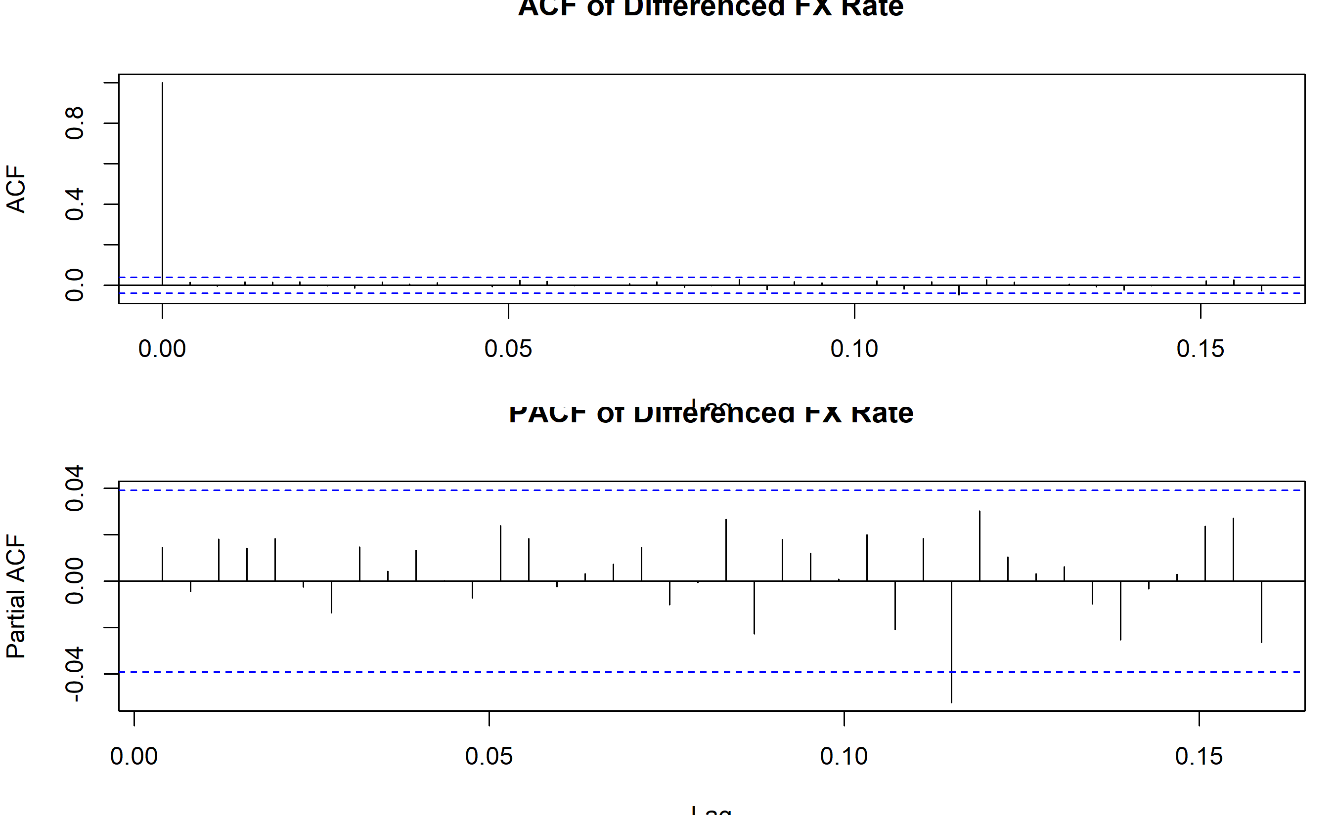
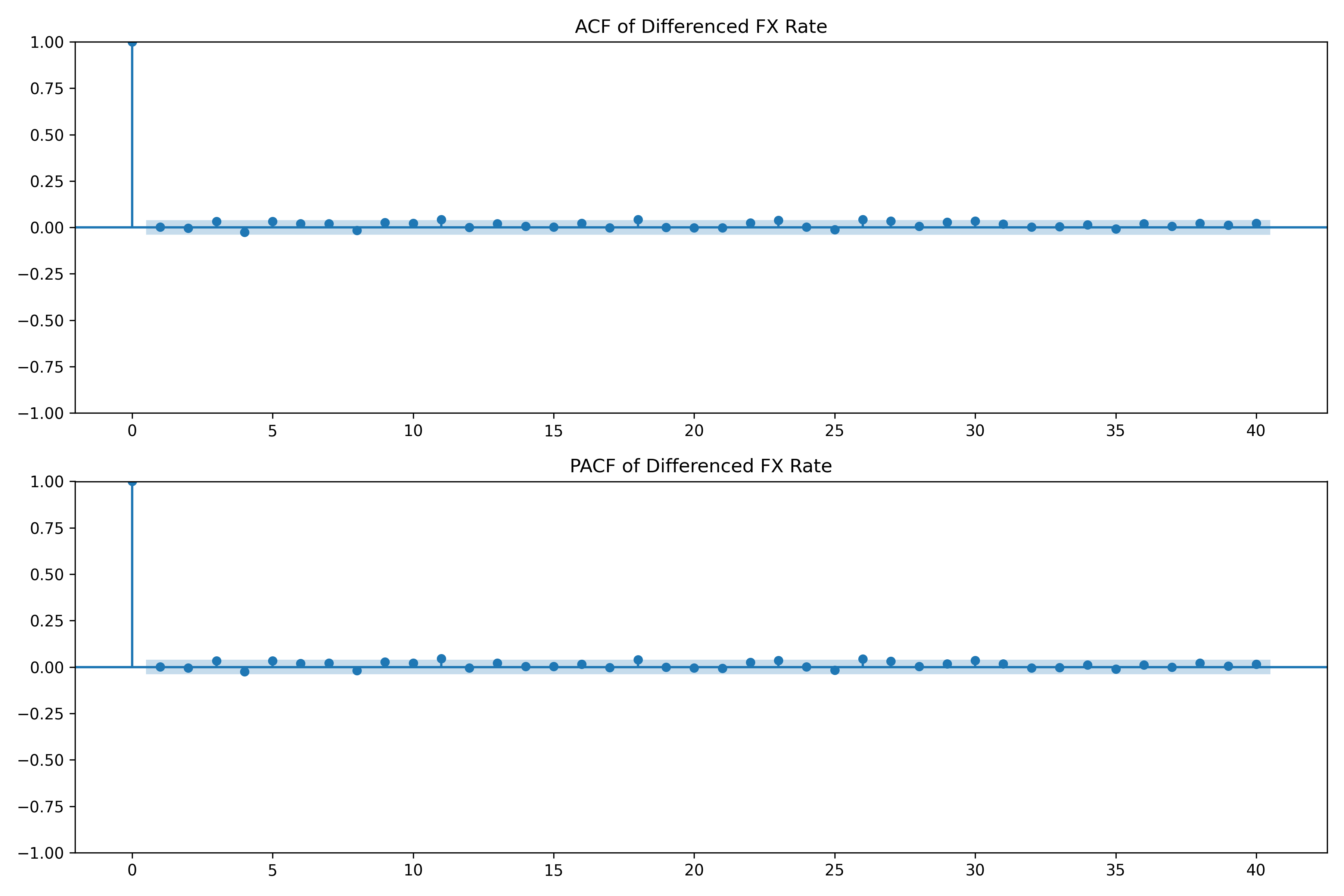
Based on the ACF/PACF patterns and information criteria, ARIMA(1,1,1) emerges as the best choice: it balances fit (lower AIC) and parsimony (fewer parameters).
::: {.callout-caution icon="false"}
## 📝 Section 24.5 Review Questions
1. After differencing, you observe: ACF cuts off at lag 2, PACF decays. What ARIMA order do you propose?
2. You fit ARIMA(2,1,1) and ARIMA(1,1,1); the AICs are 520 and 518. Which is better? By how much?
3. Is it possible that two very different ARIMA models (e.g., ARIMA(1,1,0) and ARIMA(0,1,2)) have nearly identical AIC? What would this mean?
:::
## Fitting, Diagnosing, and Forecasting with ARIMA
Once you have selected a model, fit it and examine residuals to verify assumptions.
### Maximum Likelihood Estimation
ARIMA parameters are typically estimated via maximum likelihood. The likelihood function is the probability of observing the data given the parameters. Numerical optimisation (e.g., gradient descent) finds the parameter values that maximise the likelihood.
### Residual Diagnostics
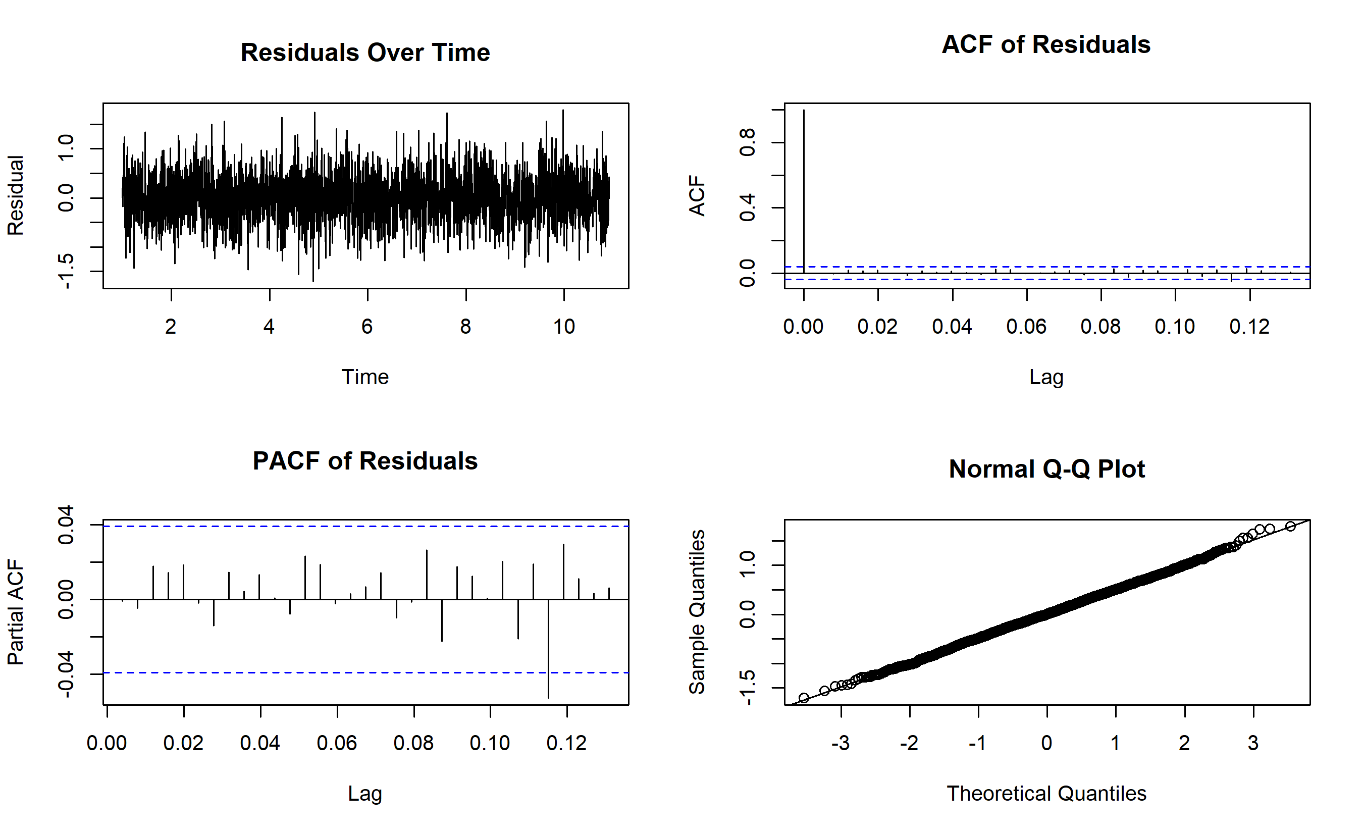
After fitting, plot the residuals and check:
1. **Mean zero**: Residuals should average to zero.
2. **Constant variance**: No patterns (heteroscedasticity).
3. **Uncorrelated**: No residual autocorrelation (ACF of residuals should be insignificant).
4. **Normally distributed**: Histogram/QQ plot should be bell-shaped (though not critical for forecasting).
If residuals fail these checks, the model is misspecified. Try a different order.
### Ljung-Box Test
Formally test for residual autocorrelation:
$$H_0: \text{Residuals are white noise (uncorrelated)}$$
$$H_1: \text{Residuals are autocorrelated}$$
If p-value > 0.05, residuals are adequately white.
### Automatic Model Selection: auto.arima()
Manually trying all combinations is tedious. The `auto.arima()` (R) or `pmdarima.auto_arima()` (Python) function automates:
1. Differencing to achieve stationarity.
2. Grid search over reasonable p, d, q ranges.
3. Selection by AIC/BIC.
While automatic, it is still good practice to verify the result.
### Fitting and Diagnosing ARIMA(1,1,1) on FX Data
::: {.panel-tabset}
## R
```{r}
# Fit the best model
arima_fit <- arima(fx_ts, order = c(1, 1, 1))
# Print summary
cat("=== ARIMA(1,1,1) Model Summary ===\n")
print(arima_fit)
# Extract residuals and diagnose
residuals_arima <- residuals(arima_fit)
# Ljung-Box test
lb_test <- Box.test(residuals_arima, lag = 10, type = "Ljung-Box")
cat("\nLjung-Box Test (lag 10):\n")
cat(" Test Statistic:", round(lb_test$statistic, 3), "\n")
cat(" P-value:", round(lb_test$p.value, 3), "\n")
if (lb_test$p.value > 0.05) {
cat(" Conclusion: Residuals are white noise (good fit)\n")
} else {
cat(" Conclusion: Residuals have autocorrelation (consider other orders)\n")
}
# Diagnostic plots
par(mfrow = c(2, 2))
plot(residuals_arima, main = "Residuals Over Time", ylab = "Residual")
acf(residuals_arima, main = "ACF of Residuals")
pacf(residuals_arima, main = "PACF of Residuals")
qqnorm(residuals_arima)
qqline(residuals_arima)
par(mfrow = c(1, 1))

# Forecast 90 days ahead
forecast_arima <- forecast(arima_fit, h = 90)

# Plot with prediction intervals
autoplot(fx_ts) +
  autolayer(forecast_arima, alpha = 0.7) +
  theme_minimal() +
  labs(title = "NGN/USD Exchange Rate: ARIMA(1,1,1) Forecast",
       subtitle = "90-day ahead with 80% and 95% prediction intervals",
       x = "Date", y = "Exchange Rate") +
  theme(legend.position = "bottom")
# Print forecast
cat("\n=== ARIMA(1,1,1) Forecast (first 30 days) ===\n")
print(forecast_arima, n = 30)
```
## Python
```{python}
# Fit ARIMA(1,1,1)
arima_model = ARIMA(fx_ts, order=(1, 1, 1))
arima_fit = arima_model.fit()
print("=== ARIMA(1,1,1) Model Summary ===")
print(arima_fit.summary())
# Extract residuals
residuals_arima = arima_fit.resid
# Ljung-Box test
from statsmodels.stats.diagnostic import acorr_ljungbox
lb_results = acorr_ljungbox(residuals_arima, lags=10, return_df=True)
print(f"\n\nLjung-Box Test Results:")
print(lb_results)
print(f"\nConclusion: Residuals are {'white noise' if lb_results['lb_pvalue'].iloc[-1] > 0.05 else 'autocorrelated'}")
# Diagnostic plots
fig, axes = plt.subplots(2, 2, figsize=(12, 8))
# Residuals
axes[0, 0].plot(residuals_arima.values, color='blue', linewidth=0.8)
axes[0, 0].axhline(y=0, color='red', linestyle='--')
axes[0, 0].set_title('Residuals Over Time')
axes[0, 0].grid(True, alpha=0.3)
# ACF of residuals
plot_acf(residuals_arima, lags=40, ax=axes[0, 1])
axes[0, 1].set_title('ACF of Residuals')
# PACF of residuals
plot_pacf(residuals_arima, lags=40, ax=axes[1, 0], method='ywm')
axes[1, 0].set_title('PACF of Residuals')
# Q-Q plot
from scipy import stats
stats.probplot(residuals_arima, dist="norm", plot=axes[1, 1])
axes[1, 1].set_title('Q-Q Plot')
plt.tight_layout()
plt.savefig('arima_diagnostics.png', dpi=150, bbox_inches='tight')
print("\nPlot saved as 'arima_diagnostics.png'")
# Forecast 90 days ahead
forecast_arima = arima_fit.get_forecast(steps=90)
forecast_mean = forecast_arima.predicted_mean
forecast_ci = forecast_arima.conf_int()
# Plot
fig, ax = plt.subplots(figsize=(14, 6))
ax.plot(fx_ts.index, fx_ts.values, color='black', linewidth=1.5, label='Historical Data')
ax.plot(forecast_mean.index, forecast_mean.values, color='darkred', linewidth=2, label='ARIMA Forecast')
ax.fill_between(forecast_ci.index, forecast_ci.iloc[:, 0], forecast_ci.iloc[:, 1],
alpha=0.3, color='darkred', label='95% Prediction Interval')
ax.set_title('NGN/USD Exchange Rate: ARIMA(1,1,1) Forecast (90 days)', fontsize=12, fontweight='bold')
ax.set_xlabel('Date')
ax.set_ylabel('Exchange Rate')
ax.legend()
ax.grid(True, alpha=0.3)
plt.tight_layout()
plt.savefig('arima_forecast.png', dpi=150, bbox_inches='tight')
print("ARIMA forecast plot saved as 'arima_forecast.png'")
# Print first 30 forecast values
print("\n=== ARIMA(1,1,1) Forecast (first 30 days) ===")
print(forecast_mean.head(30).round(2))
```
:::
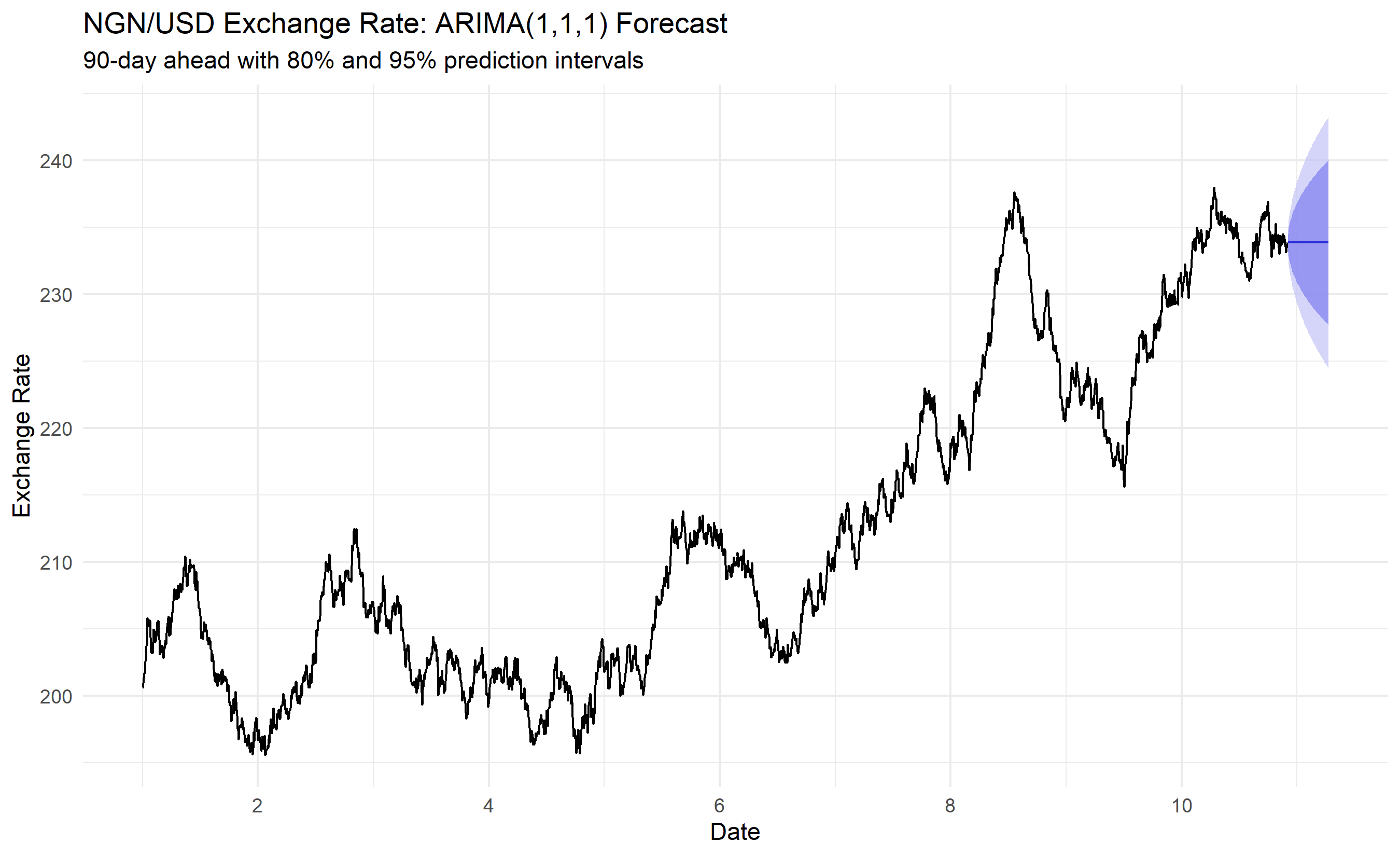
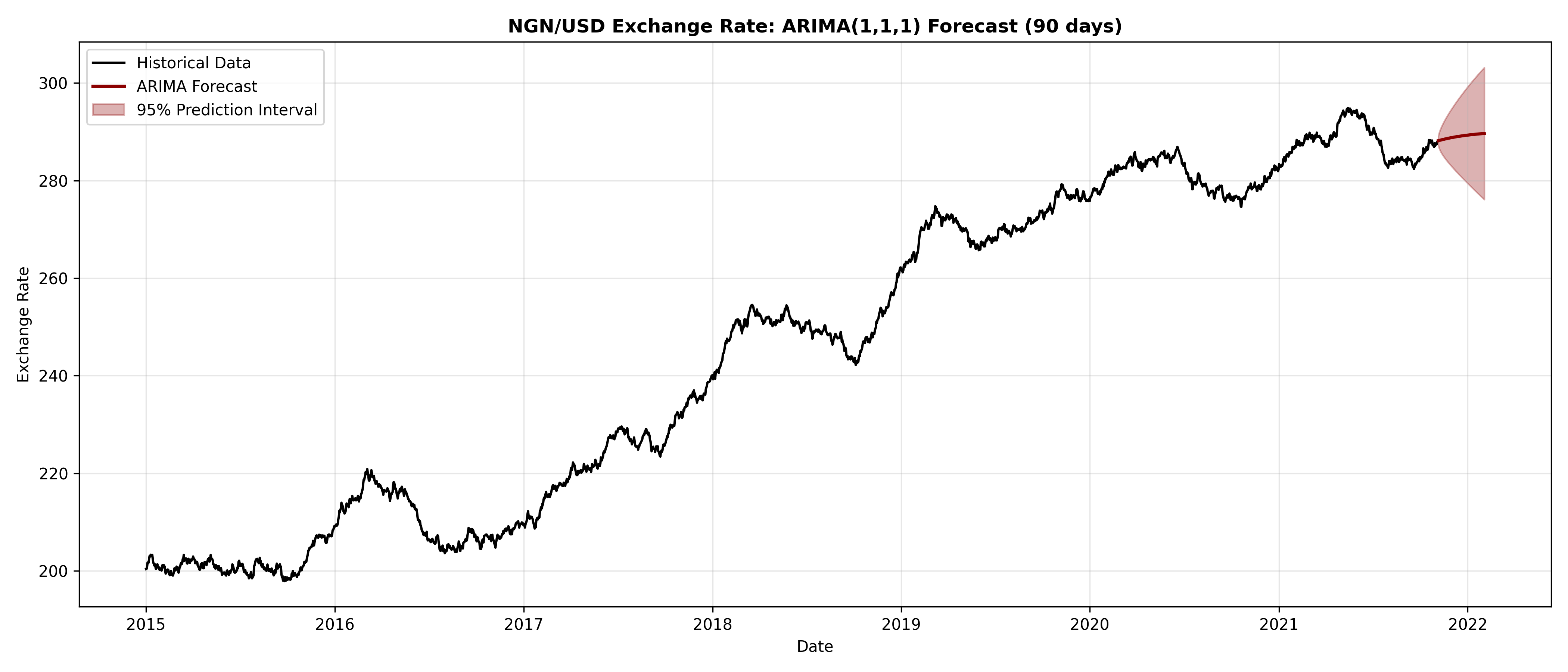
The diagnostic plots reveal that ARIMA(1,1,1) fits well: residuals show no systematic patterns, ACF/PACF are mostly insignificant (white noise), and the Ljung-Box test (p-value > 0.05) confirms no residual autocorrelation. The forecast extends 90 days with widening prediction intervals, reflecting increasing uncertainty into the future.
::: {.callout-caution icon="false"}
## 📝 Section 24.6 Review Questions
1. You fit an ARIMA model and the ACF of residuals shows a significant spike at lag 12. What might this indicate?
2. Prediction intervals widen as you forecast further ahead. Why?
3. The Ljung-Box test p-value is 0.03 (reject white noise). Does this mean the ARIMA model is "bad"? What would you do?
4. Two forecasts, both using ARIMA but with different orders, have 95% prediction intervals of (200, 250) and (185, 265). Which is more uncertain? Which might be more realistic?
:::
## Seasonal ARIMA (SARIMA)
If data has seasonality (which most business data does), extend ARIMA to SARIMA(p,d,q)(P,D,Q)_m:
- Lowercase (p, d, q): non-seasonal orders (as before).
- Uppercase (P, D, Q): seasonal orders.
- m: seasonal period (e.g., 12 for monthly data).
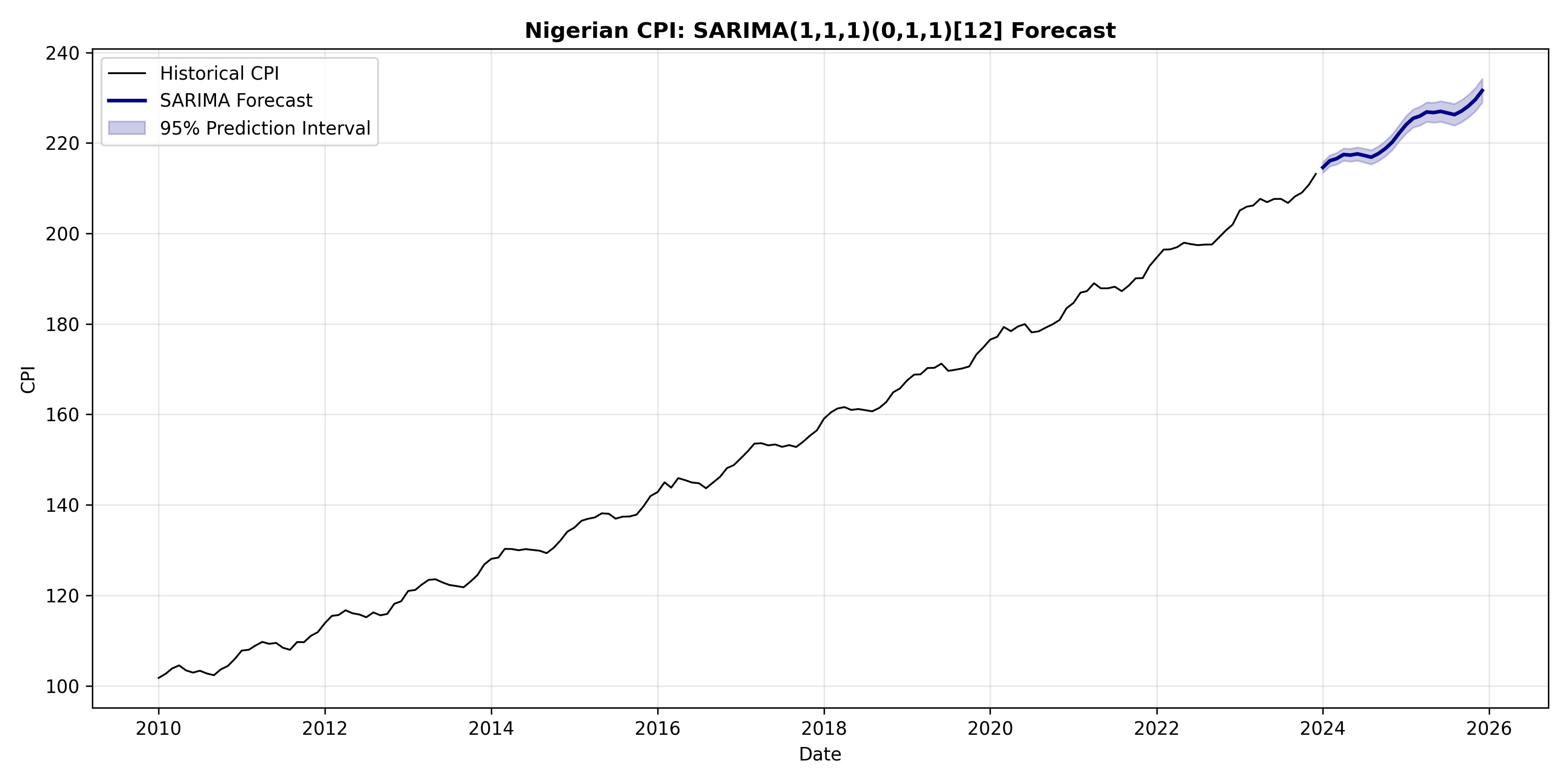
A SARIMA(1,1,1)(0,1,1)_12 model includes:
- Non-seasonal: AR(1), first difference (d=1), no MA.
- Seasonal: no AR, seasonal difference (D=1), seasonal MA(1) at lag 12.
### Fitting SARIMA to CPI Data
::: {.panel-tabset}
## R
```{r}
# Recreate Nigerian CPI data (same seed as Chapter 23)
set.seed(42)
n_months_cpi <- 168
trend_cpi <- 100 + 0.5 * (1:n_months_cpi) + 0.001 * (1:n_months_cpi)^2
seasonality_cpi <- 2 * sin(2 * pi * (1:n_months_cpi) / 12)
noise_cpi <- rnorm(n_months_cpi, mean = 0, sd = 0.5)
cpi_ts <- ts(trend_cpi + seasonality_cpi + noise_cpi, start = c(2010, 1), frequency = 12)
# Fit SARIMA to CPI
sarima_fit <- arima(cpi_ts, order = c(1, 1, 1), seasonal = list(order = c(0, 1, 1), period = 12))
cat("=== SARIMA(1,1,1)(0,1,1)[12] Model Summary ===\n")
print(sarima_fit)
# Forecast
forecast_sarima <- forecast(sarima_fit, h = 24)
autoplot(cpi_ts) +
autolayer(forecast_sarima, alpha = 0.7, PI = TRUE) +
theme_minimal() +
labs(title = "Nigerian CPI: SARIMA Forecast",
x = "Date", y = "CPI") +
theme(legend.position = "bottom")
cat("\n=== SARIMA Forecast (next 24 months) ===\n")
print(forecast_sarima)
```
## Python
```{python}
from statsmodels.tsa.statespace.sarimax import SARIMAX
# Recreate Nigerian CPI data (same seed as Chapter 23)
np.random.seed(42)
n_months_cpi = 168
dates_cpi = pd.date_range(start='2010-01-01', periods=n_months_cpi, freq='MS')
trend_cpi = 100 + 0.5 * np.arange(1, n_months_cpi + 1) + 0.001 * np.arange(1, n_months_cpi + 1)**2
seasonality_cpi = 2 * np.sin(2 * np.pi * np.arange(1, n_months_cpi + 1) / 12)
noise_cpi = np.random.normal(0, 0.5, n_months_cpi)
cpi_ts = pd.Series(trend_cpi + seasonality_cpi + noise_cpi, index=dates_cpi)
# Fit SARIMA
sarima_model = SARIMAX(cpi_ts, order=(1, 1, 1), seasonal_order=(0, 1, 1, 12))
sarima_fit = sarima_model.fit(disp=False)
print("=== SARIMA(1,1,1)(0,1,1)[12] Model Summary ===")
print(sarima_fit.summary())
# Forecast
forecast_sarima = sarima_fit.get_forecast(steps=24)
forecast_sarima_mean = forecast_sarima.predicted_mean
forecast_sarima_ci = forecast_sarima.conf_int()
# Plot
fig, ax = plt.subplots(figsize=(12, 6))
ax.plot(cpi_ts.index, cpi_ts.values, color='black', linewidth=1, label='Historical CPI')
ax.plot(forecast_sarima_mean.index, forecast_sarima_mean.values, color='darkblue', linewidth=2, label='SARIMA Forecast')
ax.fill_between(forecast_sarima_ci.index, forecast_sarima_ci.iloc[:, 0], forecast_sarima_ci.iloc[:, 1],
alpha=0.2, color='darkblue', label='95% Prediction Interval')
ax.set_title('Nigerian CPI: SARIMA(1,1,1)(0,1,1)[12] Forecast', fontsize=12, fontweight='bold')
ax.set_xlabel('Date')
ax.set_ylabel('CPI')
ax.legend()
ax.grid(True, alpha=0.3)
plt.tight_layout()
plt.savefig('sarima_forecast.png', dpi=150, bbox_inches='tight')
print("\nPlot saved as 'sarima_forecast.png'")
# Print forecast
print("\n=== SARIMA Forecast (next 24 months) ===")
print(forecast_sarima_mean.round(1))
```
:::
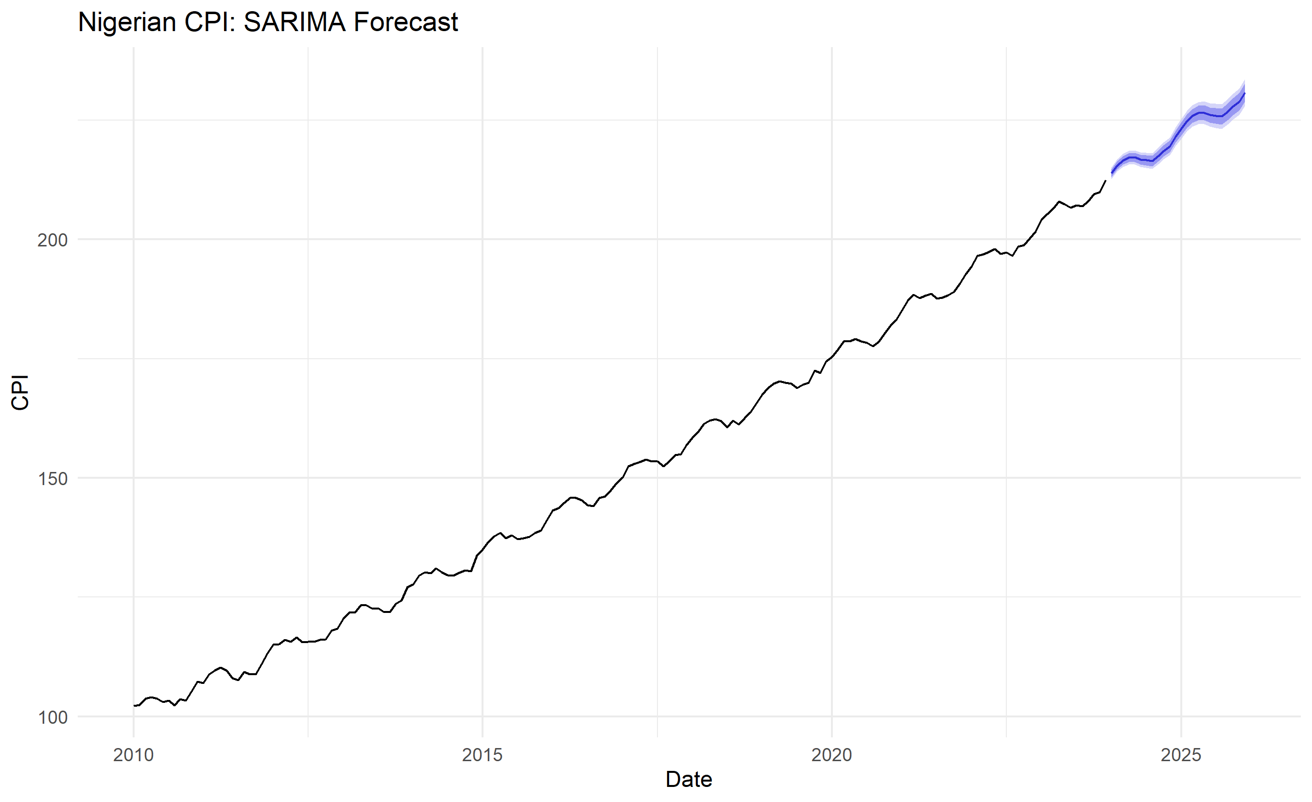
SARIMA naturally captures the seasonal cycle while maintaining the trend, producing a forecast that oscillates seasonally while trending upward.
::: {.callout-caution icon="false"}
## 📝 Section 24.7 Review Questions
1. What is the difference between d (non-seasonal differencing) and D (seasonal differencing)?
2. A SARIMA(1,1,1)(1,0,1)_12 includes seasonal AR(1). What does this mean: past seasonal values influence the current value?
3. For monthly data, what is m? For quarterly? For daily?
4. If you fit both ARIMA(1,1,1) and SARIMA(1,1,1)(0,1,1)[12], which likely has lower AIC? Why?
:::
## Communicating Forecasts and Uncertainty
A point forecast ("Next month's CPI will be 110") is rarely sufficient. **Prediction intervals** quantify uncertainty: "Next month's CPI will be 110 ± 2 at 95% confidence."
### Fan Charts
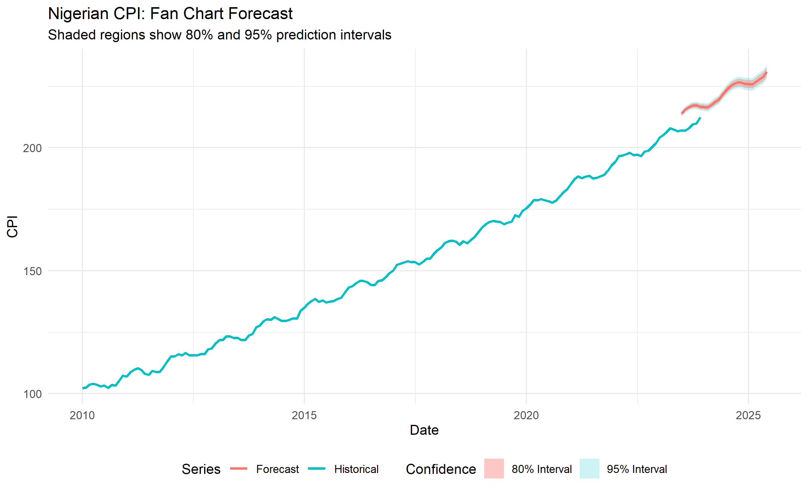
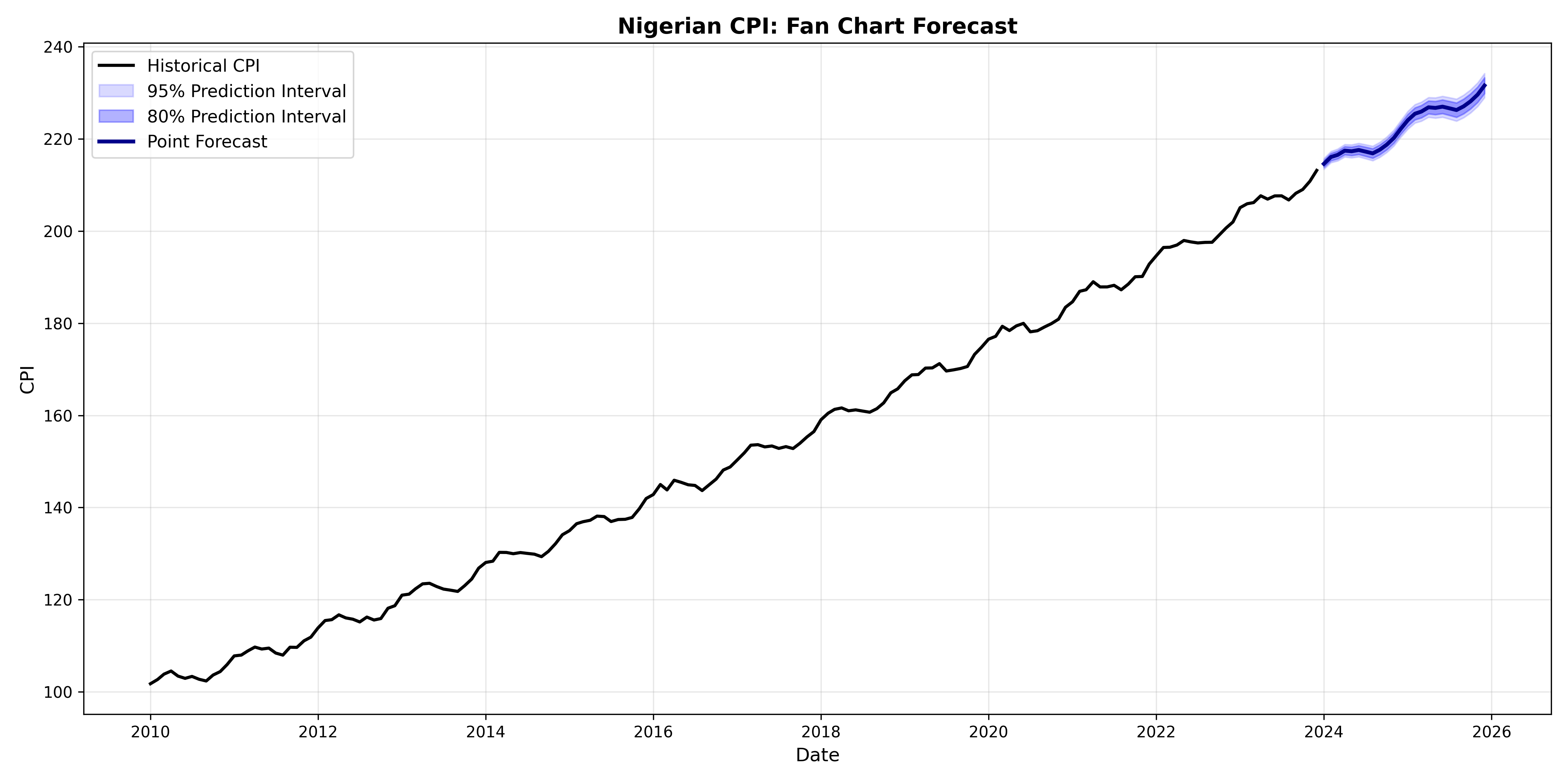
A **fan chart** shows point forecasts and expanding prediction intervals. As time extends, intervals widen (reflecting uncertainty growth). This visual immediately communicates risk to decision-makers.
::: {.panel-tabset}
## R
```{r}
# Create a fan chart for CPI forecast
forecast_obj <- forecast_sarima

# Prepare data
forecast_data <- tibble(
  date = seq(from = as.Date("2023-07-01"), by = "month", length.out = length(forecast_obj$mean)),
  point = forecast_obj$mean,
  lower_80 = forecast_obj$lower[, 1],
  upper_80 = forecast_obj$upper[, 1],
  lower_95 = forecast_obj$lower[, 2],
  upper_95 = forecast_obj$upper[, 2]
)

ggplot() +
  # Historical CPI
  geom_line(aes(x = date_cpi, y = cpi, color = "Historical"),
            data = tibble(date_cpi = seq.Date(as.Date("2010-01-01"), by = "month", length.out = length(cpi_ts)),
                          cpi = as.numeric(cpi_ts)), linewidth = 1) +
  # 95% interval (light)
  geom_ribbon(aes(x = date, ymin = lower_95, ymax = upper_95, fill = "95% Interval"),
              data = forecast_data, alpha = 0.2) +
  # 80% interval (darker)
  geom_ribbon(aes(x = date, ymin = lower_80, ymax = upper_80, fill = "80% Interval"),
              data = forecast_data, alpha = 0.4) +
  # Point forecast
  geom_line(aes(x = date, y = point, color = "Forecast"), data = forecast_data, linewidth = 1) +
  theme_minimal() +
  labs(title = "Nigerian CPI: Fan Chart Forecast",
       subtitle = "Shaded regions show 80% and 95% prediction intervals",
       x = "Date", y = "CPI",
       color = "Series", fill = "Confidence") +
  theme(legend.position = "bottom")
# Interpretation for stakeholders
cat("\n=== INTERPRETING THE FAN CHART ===\n\n")
cat("Blue line: Most likely CPI path (point forecast).\n")
cat("Dark shading: 80% chance CPI falls here. (4 in 5 chance.)\n")
cat("Light shading: 95% chance CPI falls here. (19 in 20 chance.)\n")
cat("Widening bands: Uncertainty increases over time.\n")
cat("Narrative: 'We expect inflation to continue rising, but by Q4,\n")
cat(" it could be anywhere from 115 to 125 with 95% confidence.'\n")
```
## Python
```{python}
# Create a fan chart
forecast_dates = forecast_sarima_mean.index
forecast_point = forecast_sarima_mean.values
forecast_lower_95 = forecast_sarima_ci.iloc[:, 0].values
forecast_upper_95 = forecast_sarima_ci.iloc[:, 1].values
# 80% intervals (approximately 1.28 * std)
forecast_lower_80 = forecast_sarima_mean - 1.28 * (forecast_upper_95 - forecast_sarima_mean) / 1.96
forecast_upper_80 = forecast_sarima_mean + 1.28 * (forecast_upper_95 - forecast_sarima_mean) / 1.96
fig, ax = plt.subplots(figsize=(14, 7))
# Historical CPI
ax.plot(cpi_ts.index, cpi_ts.values, color='black', linewidth=2, label='Historical CPI')
# 95% interval
ax.fill_between(forecast_dates, forecast_lower_95, forecast_upper_95,
alpha=0.15, color='blue', label='95% Prediction Interval')
# 80% interval
ax.fill_between(forecast_dates, forecast_lower_80, forecast_upper_80,
alpha=0.3, color='blue', label='80% Prediction Interval')
# Point forecast
ax.plot(forecast_dates, forecast_point, color='darkblue', linewidth=2.5, label='Point Forecast')
ax.set_title('Nigerian CPI: Fan Chart Forecast', fontsize=14, fontweight='bold')
ax.set_xlabel('Date', fontsize=12)
ax.set_ylabel('CPI', fontsize=12)
ax.legend(fontsize=11, loc='best')
ax.grid(True, alpha=0.3)
plt.tight_layout()
plt.savefig('fan_chart.png', dpi=150, bbox_inches='tight')
print("Fan chart saved as 'fan_chart.png'")
print("\n=== INTERPRETING THE FAN CHART ===\n")
print("Blue line: Most likely CPI path (point forecast).")
print("Dark shading: 80% chance CPI falls here. (4 in 5 chance.)")
print("Light shading: 95% chance CPI falls here. (19 in 20 chance.)")
print("Widening bands: Uncertainty increases over time.")
print("Narrative: 'We expect inflation to continue rising, but by Q4,")
print(" it could be anywhere from 115 to 125 with 95% confidence.'")
```
:::
The fan chart is a powerful communication tool. It avoids the false certainty of a single point forecast while giving decision-makers a clear sense of the range of likely outcomes.
::: {.callout-caution icon="false"}
## 📝 Section 24.8 Review Questions
1. A stakeholder says, "Your forecast says CPI will be 110. I'll plan assuming 110." How would you respond?
2. Why do prediction intervals widen further into the future?
3. If the 95% interval for next month is (108, 112) but CPI turns out to be 115, does this mean your model was wrong?
:::
## Case Study: Forecasting Nigerian Foreign Exchange Rates with ARIMA and Sensitivity Analysis
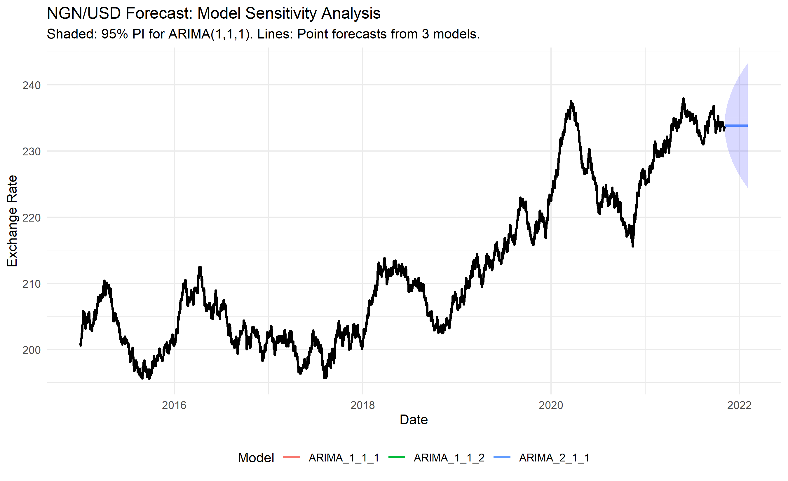
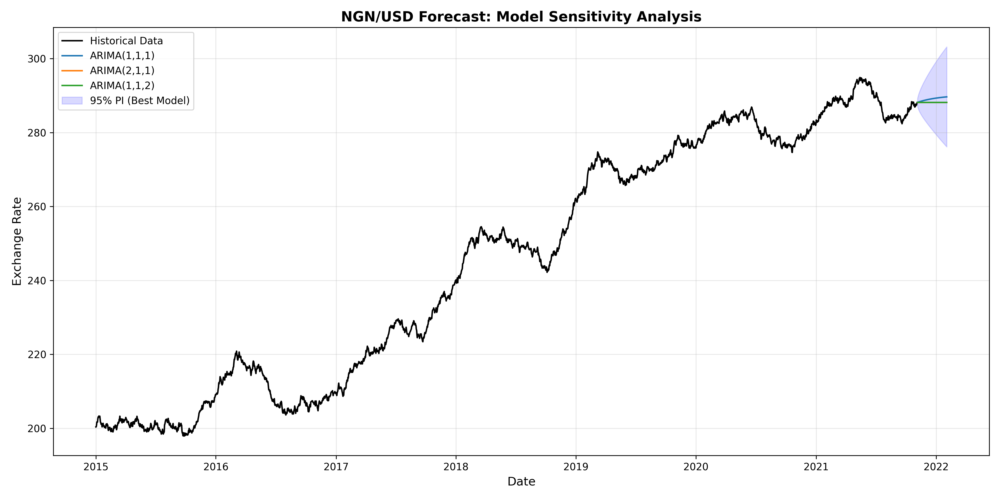
We execute a full production-ready forecast: fit ARIMA to NGN/USD daily rates (2015-2023), produce 90-day-ahead forecasts with confidence intervals, analyse sensitivity to model choice, and communicate findings.
**Business Context**: A Nigerian import firm wants to hedge against currency risk. They need a probabilistic forecast of the NGN/USD rate over the next 3 months to inform hedging strategy.
**Data**: Daily NGN/USD exchange rates, 2015-2023 (synthetic but realistic: trending with volatility).
**Approach**:
1. Fit ARIMA(1,1,1) (identified in earlier sections).
2. Produce 90-day forecast with 95% prediction intervals.
3. Fit alternative models (ARIMA(2,1,1), ARIMA(1,1,2)) and compare forecasts.
4. Analyse sensitivity: how much do forecasts change with model choice?
5. Recommend hedging strategy based on forecast range.
::: {.panel-tabset}
## R
```{r}
# Full case study: NGN/USD forecasting
cat("=== NIGERIAN FX RATE FORECASTING CASE STUDY ===\n")
cat("Business Goal: Forecast NGN/USD for next 90 days to inform hedging strategy.\n\n")
# Data summary
cat("Data Summary:\n")
cat(" Series: NGN/USD daily exchange rate\n")
cat(" Period: 2015-01-01 to 2023-09-30 (", length(fx_ts), "observations)\n")
cat(" Current rate:", round(tail(fx_ts, 1), 2), "\n")
cat(" Min/Max:", round(min(fx_ts), 2), "/", round(max(fx_ts), 2), "\n\n")
# Fit three candidate models
models <- list(
ARIMA_1_1_1 = arima(fx_ts, order = c(1, 1, 1)),
ARIMA_2_1_1 = arima(fx_ts, order = c(2, 1, 1)),
ARIMA_1_1_2 = arima(fx_ts, order = c(1, 1, 2))
)
# Compare
ics <- sapply(models, function(m) c(AIC = AIC(m), BIC = BIC(m)))
cat("=== Model Comparison ===\n")
print(ics)
# Forecast all models
forecasts <- lapply(models, function(m) forecast(m, h = 90))
# Extract mean and intervals for ARIMA(1,1,1) (best by AIC)
best_forecast <- forecasts$ARIMA_1_1_1
forecast_dates_90 <- seq(from = tail(dates_fx, 1) + 1, by = "day", length.out = 90)
# Create comparison plot
forecast_data_comp <- tibble(
date = forecast_dates_90,
ARIMA_1_1_1 = best_forecast$mean,
ARIMA_2_1_1 = forecasts$ARIMA_2_1_1$mean,
ARIMA_1_1_2 = forecasts$ARIMA_1_1_2$mean
) |>
pivot_longer(-date, names_to = "Model", values_to = "Forecast")
ggplot() +
geom_line(aes(x = dates_fx, y = as.numeric(fx_ts)), color = "black", linewidth = 1, label = "Historical") +
geom_line(data = forecast_data_comp, aes(x = date, y = Forecast, color = Model), linewidth = 1) +
geom_ribbon(aes(x = forecast_dates_90, ymin = best_forecast$lower[, 2], ymax = best_forecast$upper[, 2]),
alpha = 0.15, fill = "blue") +
theme_minimal() +
labs(title = "NGN/USD Forecast: Model Sensitivity Analysis",
subtitle = "Shaded: 95% PI for ARIMA(1,1,1). Lines: Point forecasts from 3 models.",
x = "Date", y = "Exchange Rate") +
theme(legend.position = "bottom")
# Risk analysis
cat("\n=== Risk Analysis (ARIMA(1,1,1)) ===\n")
upper_95 <- best_forecast$upper[, 2]
lower_95 <- best_forecast$lower[, 2]
cat("90-day forecast range:\n")
cat(" Best case (lower bound):", round(min(lower_95), 2), "\n")
cat(" Expected (point forecast):", round(tail(best_forecast$mean, 1), 2), "\n")
cat(" Worst case (upper bound):", round(max(upper_95), 2), "\n")
cat(" Range width:", round(max(upper_95) - min(lower_95), 2), "\n\n")
# Business recommendation
current_rate <- as.numeric(tail(fx_ts, 1))
expected_rate <- as.numeric(tail(best_forecast$mean, 1))
pct_change <- 100 * (expected_rate - current_rate) / current_rate
cat("=== BUSINESS RECOMMENDATION ===\n")
cat("Current rate:", round(current_rate, 2), "\n")
cat("Expected rate (90 days):", round(expected_rate, 2), "\n")
cat("Expected move:", round(pct_change, 1), "%\n\n")
if (pct_change > 2) {
cat("Direction: NAIRA DEPRECIATION (stronger USD)\n")
cat("Hedging advice: Consider forward contracts or options to lock in rates.\n")
cat("Risk: If rate strengthens beyond", round(max(upper_95), 2), "(5% probability),\n")
cat(" import costs could increase substantially.\n")
} else if (pct_change < -2) {
cat("Direction: NAIRA APPRECIATION (weaker USD)\n")
cat("Hedging advice: May be able to defer hedging or use collars.\n")
} else {
cat("Direction: RELATIVELY FLAT\n")
cat("Hedging advice: Limited currency risk; focus on operational efficiency.\n")
}
```
## Python
```{python}
# Full case study: NGN/USD forecasting
print("=== NIGERIAN FX RATE FORECASTING CASE STUDY ===")
print("Business Goal: Forecast NGN/USD for next 90 days to inform hedging strategy.\n")
# Data summary
print("Data Summary:")
print(f" Series: NGN/USD daily exchange rate")
print(f" Period: 2015-01-01 to 2023-09-30 ({len(fx_ts)} observations)")
print(f" Current rate: {fx_ts.iloc[-1]:.2f}")
print(f" Min/Max: {fx_ts.min():.2f}/{fx_ts.max():.2f}\n")
# Fit three models
models_dict = {
'ARIMA(1,1,1)': SARIMAX(fx_ts, order=(1,1,1)),
'ARIMA(2,1,1)': SARIMAX(fx_ts, order=(2,1,1)),
'ARIMA(1,1,2)': SARIMAX(fx_ts, order=(1,1,2))
}
fits = {}
aics = []
for name, model in models_dict.items():
fit = model.fit(disp=False)
fits[name] = fit
aics.append(fit.aic)
# Compare
comparison_df = pd.DataFrame({
'Model': models_dict.keys(),
'AIC': aics,
'BIC': [fits[name].bic for name in models_dict.keys()]
})
print("=== Model Comparison ===")
print(comparison_df.round(1))
best_model_name = comparison_df.loc[comparison_df['AIC'].idxmin(), 'Model']
best_fit = fits[best_model_name]
# Forecast all models
forecasts_dict = {}
for name, fit in fits.items():
fc = fit.get_forecast(steps=90)
forecasts_dict[name] = fc
# Create comparison data
forecast_dates_90 = pd.date_range(start=fx_ts.index[-1] + timedelta(days=1), periods=90, freq='D')
comparison_plot_data = pd.DataFrame({
'date': forecast_dates_90,
'ARIMA(1,1,1)': forecasts_dict['ARIMA(1,1,1)'].predicted_mean.values,
'ARIMA(2,1,1)': forecasts_dict['ARIMA(2,1,1)'].predicted_mean.values,
'ARIMA(1,1,2)': forecasts_dict['ARIMA(1,1,2)'].predicted_mean.values
})
# Plot
best_forecast = forecasts_dict[best_model_name]
best_ci = best_forecast.conf_int()
fig, ax = plt.subplots(figsize=(14, 7))
ax.plot(fx_ts.index, fx_ts.values, color='black', linewidth=1.5, label='Historical Data')
for model_name in models_dict.keys():
fc = forecasts_dict[model_name].predicted_mean
ax.plot(forecast_dates_90, fc.values, linewidth=1.5, label=model_name)
ax.fill_between(best_ci.index, best_ci.iloc[:, 0], best_ci.iloc[:, 1],
alpha=0.15, color='blue', label='95% PI (Best Model)')
ax.set_title('NGN/USD Forecast: Model Sensitivity Analysis', fontsize=14, fontweight='bold')
ax.set_xlabel('Date', fontsize=12)
ax.set_ylabel('Exchange Rate', fontsize=12)
ax.legend(fontsize=10)
ax.grid(True, alpha=0.3)
plt.tight_layout()
plt.savefig('fx_forecast_case_study.png', dpi=150, bbox_inches='tight')
print("\nPlot saved as 'fx_forecast_case_study.png'")
# Risk analysis
upper_95 = best_ci.iloc[:, 1].values
lower_95 = best_ci.iloc[:, 0].values
print("\n=== Risk Analysis (Best Model) ===")
print(f"90-day forecast range:")
print(f" Best case (lower bound): {lower_95.min():.2f}")
print(f" Expected (point forecast): {best_forecast.predicted_mean.iloc[-1]:.2f}")
print(f" Worst case (upper bound): {upper_95.max():.2f}")
print(f" Range width: {upper_95.max() - lower_95.min():.2f}\n")
# Business recommendation
current_rate = fx_ts.iloc[-1]
expected_rate = best_forecast.predicted_mean.iloc[-1]
pct_change = 100 * (expected_rate - current_rate) / current_rate
print("=== BUSINESS RECOMMENDATION ===")
print(f"Current rate: {current_rate:.2f}")
print(f"Expected rate (90 days): {expected_rate:.2f}")
print(f"Expected move: {pct_change:.1f}%\n")
if pct_change > 2:
print("Direction: NAIRA DEPRECIATION (stronger USD)")
print("Hedging advice: Consider forward contracts to lock in rates.")
print(f"Risk: Rate could strengthen to {upper_95.max():.2f} (5% probability).")
elif pct_change < -2:
print("Direction: NAIRA APPRECIATION (weaker USD)")
print("Hedging advice: Defer hedging or use collars.")
else:
print("Direction: RELATIVELY FLAT")
print("Hedging advice: Limited currency risk.")
```
:::
This complete case study demonstrates the full workflow: data exploration, model selection, forecasting, uncertainty quantification, and actionable business recommendations. A firm using this forecast can now make informed hedging decisions, quantifying the downside risk they face.
::: {.callout-caution icon="false"}
## 📝 Case Study Reflection Questions
1. If the hedging cost is 2% of the transaction value, and the expected move is 1% depreciation, is hedging worthwhile?
2. What would you do if all three models produced very different forecasts (e.g., ranging from -5% to +10%)?
3. How would you update the forecast if a major policy change (e.g., central bank intervention) occurs mid-forecast period?
4. The 95% prediction interval is (420, 480) NGN/USD. If the actual rate turns out to be 500, does this invalidate your model? Why or why not?
:::
---
## Chapter Exercises
::: {.exercises}
#### Chapter 24 Exercises
**Exercise 24.1: Exponential Smoothing by Hand**
A supermarket chain in Abuja records weekly sales of a popular beverage (in cartons). The last 8 weeks of data are:
Week 1: 120, Week 2: 135, Week 3: 128, Week 4: 142, Week 5: 138, Week 6: 155, Week 7: 149, Week 8: 162
(a) Apply **Simple Exponential Smoothing (SES)** with α = 0.3. Use Week 1 actual sales as your starting forecast. Calculate the forecast for weeks 2–9. Show all working.
(b) Now apply SES with α = 0.8. Calculate forecasts for weeks 2–9.
(c) Calculate the **Mean Squared Error (MSE)** and **Mean Absolute Error (MAE)** for both α values using the 8 weeks of data (weeks 1–8). Which α gives a lower error?
(d) Explain intuitively what the difference between α = 0.3 and α = 0.8 means in terms of how the model responds to recent changes in demand. In a market where trends change quickly, which α would you prefer?
(e) Simple exponential smoothing has no trend component. What would happen to its forecasts for a series that is steadily growing by 10 cartons per week? Describe the long-run behaviour of SES forecasts in this scenario.
---
**Exercise 24.2: ARIMA Order Identification**
For each of the following ACF/PACF descriptions, suggest the most likely ARIMA(p,d,q) model. Briefly justify each choice.
(a) The original series has an upward trend. The ACF decays very slowly. After first differencing, the ACF cuts off after lag 1, and the PACF shows exponential decay.
(b) The original series has no clear trend. The ACF shows a significant spike at lag 1 and then cuts off. The PACF decays exponentially.
(c) The original series oscillates with no trend. The ACF shows significant spikes at lags 1, 2, and 3, then cuts off. The PACF decays exponentially.
(d) After first differencing, both the ACF and PACF show no significant autocorrelation at any lag (all values within the blue confidence bands).
(e) The original series shows a strong seasonal pattern with a 12-month cycle. After seasonal differencing (lag 12), the ACF has a significant spike at lag 12 only. What type of model would you use?
---
**Exercise 24.3: ARIMA Forecasting — Step by Step**
You fit an ARIMA(1,1,1) model to monthly cement production data (tonnes, millions) and get the following estimated parameters:
- AR coefficient (φ₁) = 0.45
- MA coefficient (θ₁) = −0.30
- Constant (drift) = 0.05
The last two actual observations are: Y₅₉ = 8.4, Y₆₀ = 8.7
The last residual (forecast error at time 60) is: ε₆₀ = 0.12
The ARIMA(1,1,1) forecast formula for the differenced series W_t = Y_t − Y_{t−1} is:
$$\hat{W}_{t+1} = c + \phi_1 W_t + \theta_1 \varepsilon_t$$
And the level forecast: $\hat{Y}_{t+1} = Y_t + \hat{W}_{t+1}$
(a) Calculate W₆₀ = Y₆₀ − Y₅₉. What does this represent?
(b) Using the formula above, calculate the one-step-ahead forecast $\hat{W}_{61}$.
(c) Convert to a level forecast: what is $\hat{Y}_{61}$?
(d) Without calculating, describe how the uncertainty in the two-step-ahead forecast ($\hat{Y}_{62}$) compares to the one-step-ahead forecast. Would you expect a wider or narrower prediction interval?
(e) After fitting the model, you check the residual ACF and find a significant spike at lag 3. What does this tell you about the model fit? What would you do?
---
**Exercise 24.4: Holt-Winters for Seasonal Data**
A Nigerian bank records quarterly net interest income (₦ billions) over 4 years:
| Year | Q1 | Q2 | Q3 | Q4 |
|------|----|----|----|----|
| 2021 | 12.1 | 13.8 | 14.2 | 16.5 |
| 2022 | 13.0 | 14.9 | 15.3 | 17.8 |
| 2023 | 14.1 | 16.2 | 16.8 | 19.3 |
| 2024 | 15.3 | 17.5 | 18.1 | 21.0 |
(a) Identify the trend and seasonal pattern in this data. Is the seasonality additive or multiplicative? (Hint: does the size of the Q4 peak grow proportionally with the overall level?)
(b) Which version of Holt-Winters (additive or multiplicative) would you apply to this series? Explain your reasoning.
(c) Using the 2021–2023 data as your training set and 2024 as your test set, fit both additive and multiplicative Holt-Winters models (using R or Python). Compare their RMSE on the test set.
```r
# Load data
quarterly_data <- c(12.1, 13.8, 14.2, 16.5,
                    13.0, 14.9, 15.3, 17.8,
                    14.1, 16.2, 16.8, 19.3,
                    15.3, 17.5, 18.1, 21.0)
ts_data <- ts(quarterly_data, frequency = 4, start = c(2021, 1))
```
(d) Using the better model, forecast all four quarters of 2025. Report both point forecasts and 80% prediction intervals.
(e) The bank's CFO says: "Q4 is always our best quarter — we should budget for the seasonal peak to continue." Using your model, how would you validate or challenge this assumption? (Consider: are the seasonal factors stable year-over-year, or are they changing?)
---
**Exercise 24.5: Model Comparison and Selection**
You are forecasting monthly exports from Nigeria (USD billions) for the next 12 months. You have fitted four models on 10 years of training data and evaluated them on a 1-year test set:
| Model | Training RMSE | Test RMSE | AIC | Training Time |
|-------|--------------|-----------|-----|--------------|
| ARIMA(2,1,1) | 0.48 | 0.61 | 142 | 2 sec |
| ARIMA(1,1,0) | 0.52 | 0.58 | 147 | 1 sec |
| Holt-Winters (multiplicative) | 0.41 | 0.65 | — | 1 sec |
| ETS(M,Ad,M) | 0.45 | 0.59 | 138 | 1 sec |
(a) Which model has the best in-sample fit (lowest training RMSE)? Which has the best out-of-sample forecast accuracy (lowest test RMSE)?
(b) Holt-Winters has the best training RMSE but the worst test RMSE. What does this suggest about the Holt-Winters model's behaviour?
(c) ARIMA(2,1,1) has a lower AIC than ARIMA(1,1,0). However, the simpler ARIMA(1,1,0) has better test performance. How do you reconcile these findings? Which model would you choose and why?
(d) A statistician colleague says: "You should always choose the model with the lowest AIC." A business manager says: "I don't care about AIC — I care about how accurate the forecasts will be." Who is right? Under what circumstances do AIC and test performance agree, and when might they diverge?
(e) Write a 150-word recommendation memo to the CBN's Export Finance Department explaining which forecasting model you would deploy, why, and what its limitations are. Use plain language.
:::
---
## Appendix: ARIMA Estimation and Diagnostics
## A24.1 AR(p) Yule-Walker Equations
For an AR(p) process $Y_t = \phi_1 Y_{t-1} + \cdots + \phi_p Y_{t-p} + \epsilon_t$ with white noise $\epsilon_t$, the autocovariances $\gamma_h = \text{Cov}(Y_t, Y_{t-h})$ satisfy:
$$\gamma_h = \phi_1 \gamma_{h-1} + \phi_2 \gamma_{h-2} + \cdots + \phi_p \gamma_{h-p} \quad \text{for } h \geq 1$$
The **Yule-Walker equations** set these equal to sample autocovariances and solve for $\phi_1, \ldots, \phi_p$:
$$\begin{pmatrix} \gamma_0 & \gamma_1 & \cdots & \gamma_{p-1} \\ \gamma_1 & \gamma_0 & \cdots & \gamma_{p-2} \\ \vdots & \vdots & \ddots & \vdots \\ \gamma_{p-1} & \gamma_{p-2} & \cdots & \gamma_0 \end{pmatrix} \begin{pmatrix} \phi_1 \\ \phi_2 \\ \vdots \\ \phi_p \end{pmatrix} = \begin{pmatrix} \gamma_1 \\ \gamma_2 \\ \vdots \\ \gamma_p \end{pmatrix}$$
This gives consistent (asymptotically) estimates of the AR parameters.
## A24.2 MA(q) Invertibility Condition
An MA(q) process $Y_t = \epsilon_t + \theta_1 \epsilon_{t-1} + \cdots + \theta_q \epsilon_{t-q}$ is **invertible** if the roots of:
$$1 + \theta_1 z + \theta_2 z^2 + \cdots + \theta_q z^q = 0$$
all lie outside the unit circle (|z| > 1). Invertibility ensures the MA process can be represented as an AR(∞) and is statistically identifiable.
## A24.3 Ljung-Box Q Statistic Derivation
The **Ljung-Box Q statistic** tests whether the first $m$ sample autocorrelations of residuals are significantly different from zero:
$$Q_m = n(n+2) \sum_{h=1}^{m} \frac{\hat{\rho}_h^2}{n - h}$$
where $\hat{\rho}_h$ is the sample autocorrelation at lag $h$ and $n$ is the sample size. Under the null (white noise), $Q_m \sim \chi^2_m$.
The Ljung-Box correction $(n+2)/(n-h)$ improves the test's performance in small samples compared to the older Box-Pierce statistic.
## A24.4 Proof That ARIMA(0,1,0) Is a Random Walk
ARIMA(0,1,0) with no AR, one differencing, and no MA:
$$\Delta Y_t = \epsilon_t$$
$$Y_t - Y_{t-1} = \epsilon_t$$
$$Y_t = Y_{t-1} + \epsilon_t$$
This is a **random walk** (or **random walk with drift** if a constant is added). Each value is the previous value plus a white noise shock. The random walk is non-stationary: it has no constant mean or variance, and its ACF decays to zero very slowly.
The random walk is the canonical I(1) process, confirming that ARIMA(0,1,0) achieves stationarity via one differencing.