---
title: "Supply Chain and Logistics Analytics"
author: "Bongo Adi"
---
```{python}
#| label: python-setup-48-supply-chain-logistics
#| include: false
import numpy as np
import pandas as pd
import matplotlib.pyplot as plt
import seaborn as sns
```
::: {.callout-note icon="false"}
## 📋 Learning Objectives
- Understand supply chain networks and the bullwhip effect
- Calculate key supply chain metrics: OTIF, on-time delivery, fill rate, perfect order rate
- Perform exploratory analysis to identify late delivery hotspots
- Build predictive models for late deliveries using machine learning
- Analyse supply chain risk: concentration risk and network resilience
- Solve vehicle routing problems (VRP) using heuristics
- Implement supply chain analytics with Nigerian FMCG case study
:::
## Why Supply Chains Break
Supply chains are networks under uncertainty. A brand manufactures products, distributes through warehouses, and delivers to retail points and end consumers. At each step, variability enters: demand fluctuates (weather, promotions, holidays), lead times vary (port delays, production downtime), quality issues arise (defective units, damage in transit). If these uncertainties are managed—inventory buffers, safety stock, multiple sourcing—the chain hums. But when assumptions break (a supplier fails, demand spikes unexpectedly), the chain fractures, and products don't reach customers on time.
The **bullwhip effect** is a well-documented phenomenon where small demand fluctuations at retail amplify upstream. If end-market demand increases by 10%, a retailer increases orders to wholesalers by 15% (to build safety stock). The wholesaler, seeing a 15% spike, increases orders to manufacturers by 25% (anticipating further growth). The manufacturer sees 25% swings and increases raw material orders by 40%. A 10% consumer demand bump becomes a 40% swing in raw material demand upstream. This amplification destabilises production planning, inflates inventory costs, and increases stockout risk when demand reverses.
In Nigeria, supply chain fragility is acute. **Apapa port congestion** (Lagos) creates unpredictable import delays (declared 10 days, actual 40 days). **Fuel scarcity** stalls logistics vehicles, delaying shipments from refineries to distributors, cascading failures downstream. **Road infrastructure** (Lagos-Ibadan expressway often congested) stretches last-mile delivery windows. **Inventory shrinkage** from theft (especially in northern Nigeria) requires larger safety stock buffers. **Customs clearance delays** (ports, land borders) create batch-level uncertainty. A pharmaceutical distributor aiming for 98% on-time delivery must account for these endemic risks.
Why analytics matters: visibility (real-time tracking), prediction (identifying which shipments will be late before they leave the warehouse), and optimisation (routing trucks to minimise delays and costs). A late shipment hurts: retail stockouts, customer complaints, contractual penalties. Reducing late delivery by 5 percentage points (97% → 92%) saves customer acquisition costs (fewer lost customers) and improves EBITDA (lower expedited shipping costs).
::: {.callout-note icon="false"}
## 📘 Theory: Supply Chain Risk and Resilience
Supply chain resilience is the ability to absorb shocks (demand spikes, supplier failures) without severe degradation. Metrics: recovery time (how fast to normal operations), loss magnitude (revenue/inventory impact during disruption). Lean supply chains (minimized inventory, single-sourcing) are efficient but fragile. Robust chains accept higher steady-state costs (dual suppliers, safety stock) to absorb shocks. Nigerian supply chains need robustness: endemic disruptions (port delays, fuel scarcity, security) are not exceptions but norms. Analytics quantifies the cost-benefit tradeoff.
:::
::: {.callout-tip icon="false"}
## 🔑 Key Metric: Bullwhip Effect Quantification
**Order Variance Amplification:**
$$\text{Bullwhip Ratio} = \frac{\text{Variance of Orders Upstream}}{\text{Variance of Demand Downstream}}$$
A ratio > 1 indicates amplification; ratio = 1.3 means a 10% demand swings becomes 13% order swings upstream.
:::
## Supply Chain Key Metrics: How Do You Know If the Chain Is Working?
You cannot improve what you cannot measure. Supply chain management has developed a set of standard metrics — numerical scorecards — that tell you, at a glance, how well goods are flowing from production to customers. Understanding these metrics is the first step to diagnosing problems and designing improvements.
**On-Time In-Full (OTIF)** is the headline number. It measures the percentage of orders that were delivered both on time AND with the exact quantity the customer ordered. Notice that both conditions must be met simultaneously. If a retailer in Kano orders 100 bags of rice and you deliver 100 bags one day late, you have failed OTIF. If you deliver 85 bags on time, you have also failed OTIF. Only a delivery of exactly 100 bags by the agreed date counts as a pass.
$$\text{OTIF} = \frac{\text{Orders delivered on time AND complete}}{\text{Total orders}} \times 100\%$$
A 98% OTIF means 2% of orders are either late, short, or both. This sounds small, but for a company shipping 10,000 orders per month, that is 200 failures per month — 200 frustrated customers, 200 potential chargebacks, 200 opportunities for a competitor to step in.
Why does OTIF matter so much? Because from the customer's perspective, a delivery is either right or wrong. A supermarket chain cannot stock its shelves with 85 bags of rice when they ordered 100. A hospital cannot safely substitute one drug for another just because the right one arrived three days late. Major retailers like Shoprite, PZ Cussons, and FMCG distributors across Nigeria now enforce OTIF clauses in supplier contracts — suppliers who consistently underperform face financial penalties or lose their listing.
**Other key metrics** that together paint a complete picture:
- **On-Time Delivery Rate (OTD):** Measures only whether the delivery arrived by the promised date, regardless of whether it was complete. A shipment of 85 bags (short) delivered on time would pass OTD but fail OTIF. Tracking OTD separately from OTIF helps identify whether problems are transport-related (timing) or warehouse-related (picking and packing errors).
- **Fill Rate:** The percentage of units in customer orders that were fulfilled from available stock without needing to back-order or delay. If a customer orders 500 units and you can ship only 430 because 70 were out of stock, your fill rate for that order is 86%. Fill rate reveals stockout problems at the warehouse level, before goods even reach the carrier.
- **Perfect Order Rate:** The most demanding metric — the percentage of orders that are correct on every single dimension: right product, right quantity, right delivery date, right documentation, and undamaged on arrival. Even a small labelling error or a cracked package counts as a failure. This is the metric pharmaceutical companies must track for regulatory compliance.
- **Cash-to-Cash Cycle Time:** This measures how long it takes for money invested in raw materials and inventory to return to the company as cash from customer payments. Shorter cycles mean less working capital tied up in the supply chain. If you pay your supplier on day 0, the goods sit in your warehouse for 30 days, you ship them on day 30, and your customer pays on day 60, your cash-to-cash cycle is 60 days — meaning you need to finance 60 days of inventory from your own resources or a credit line.
- **Inventory Turnover:** Annual sales divided by average inventory value. A turnover of 6 means the business sells and replaces its entire inventory six times per year — once every two months. Higher turnover generally means less capital tied up in stock and fresher products. But extremely high turnover can lead to stockouts if replenishment cannot keep up with demand.
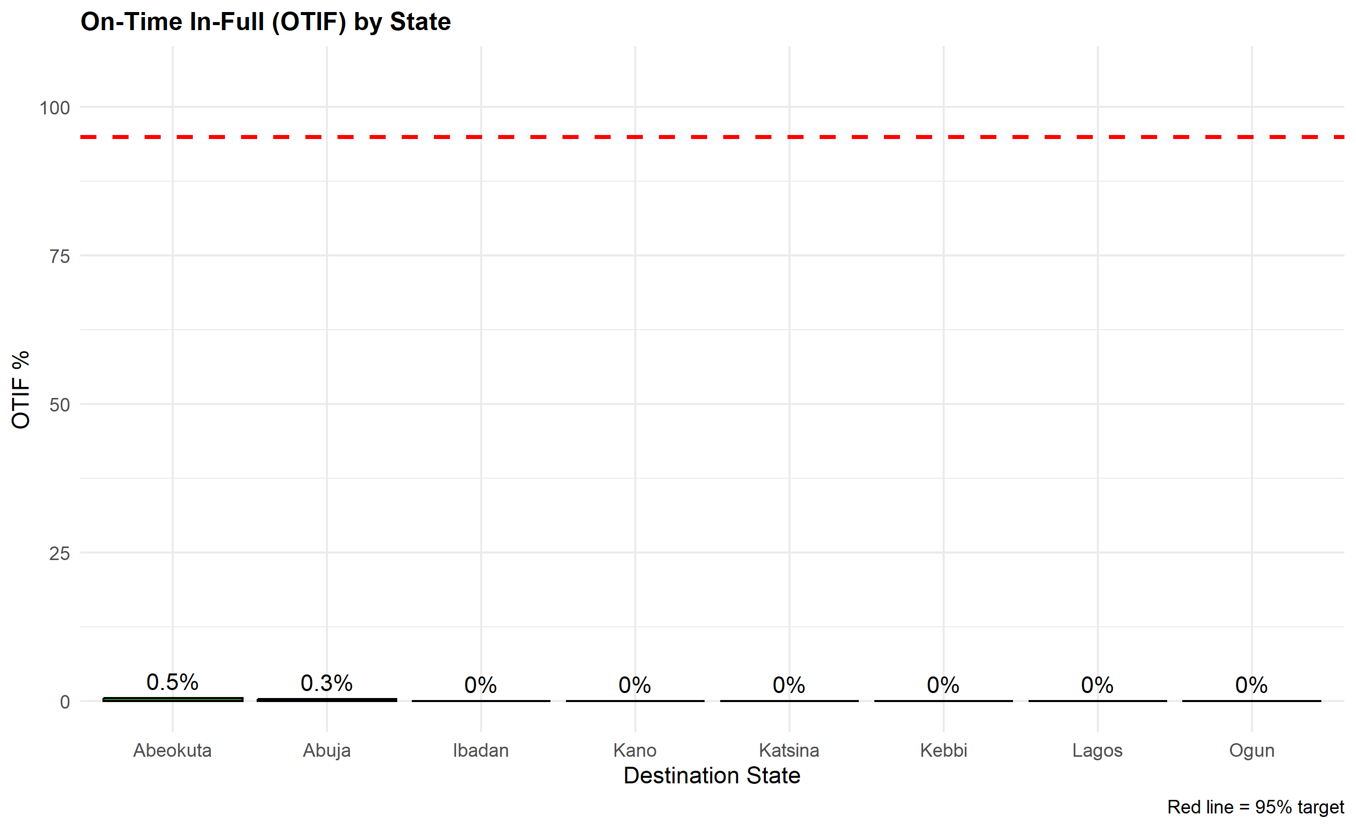
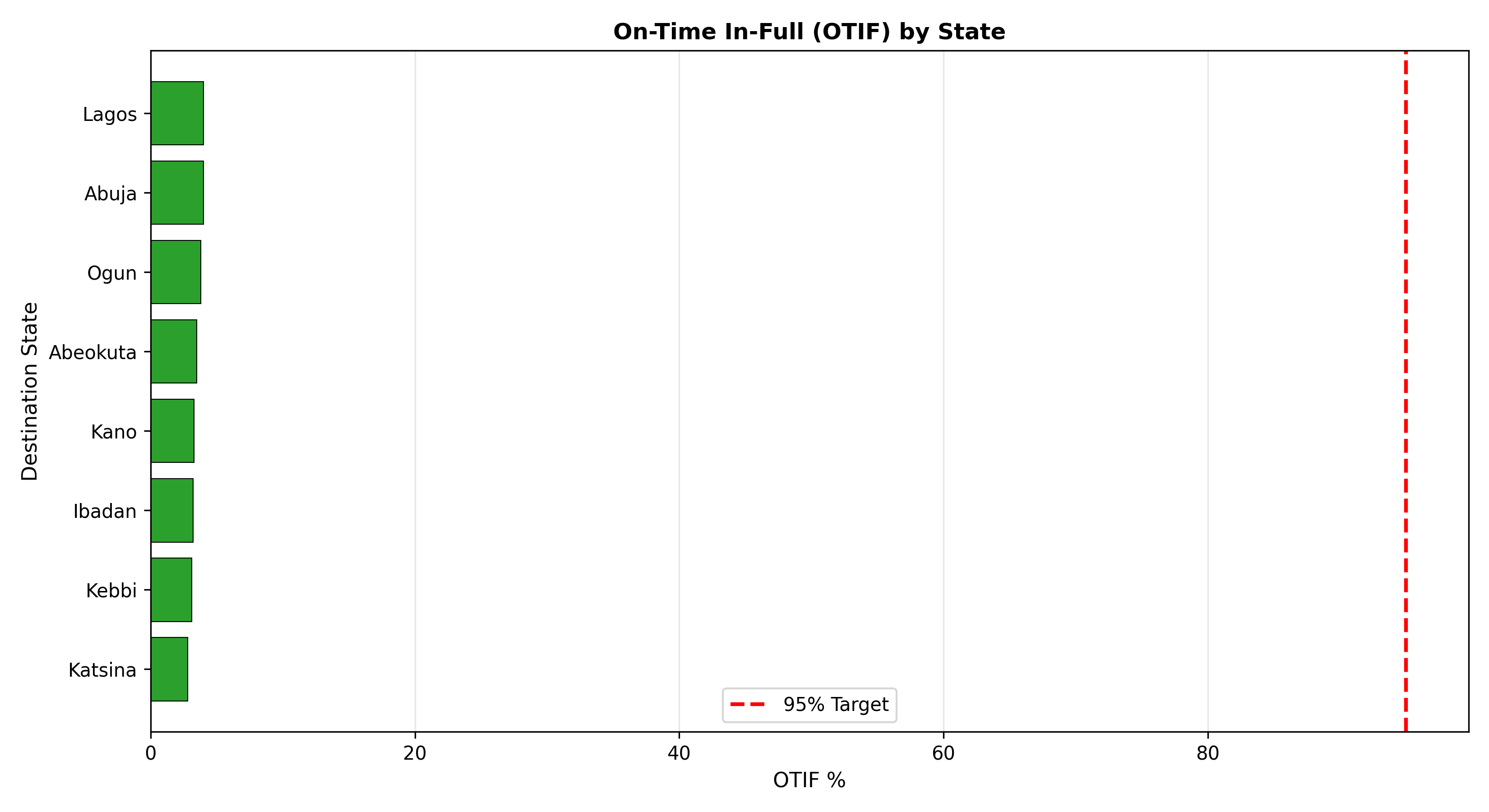
In Nigeria specifically, OTIF varies dramatically by geography and carrier. Lagos-to-Abuja routes with reliable logistics partners might achieve 94–96% OTIF on a good week. Deliveries to rural markets in Kebbi or Adamawa, over poor roads with fuel scarcity, might achieve only 65–70%. A single metric across the entire country would mask these differences. Supply chain analytics must always be broken down by route, region, carrier, and product category to identify where interventions will have the greatest impact.
::: {.callout-note icon="false"}
## 📘 Theory: OTIF and Service Level Economics
Service level (percentage of demand met from stock without delay) is chosen to balance inventory cost and stockout cost. Higher service levels require higher safety stock, increasing carrying costs. Lower service levels risk customer dissatisfaction and lost sales. The optimal service level is where marginal cost of extra inventory equals marginal benefit of avoided stockouts. Most B2B firms target 95–99% service level; retail tolerates 90–95%.
:::
::: {.panel-tabset}
## R
```{r}
#| label: ch48-supply-chain-metrics
#| message: false
#| warning: false
library(tidyverse)
library(ggplot2)
library(maps)
# Synthetic Nigerian FMCG distribution data: 50,000 order lines
set.seed(7038)
n_orders <- 50000
supply_data <- tibble(
Order_ID = rep(1:5000, each = 10), # 5,000 orders × 10 line items
Order_Date = rep(as.Date("2024-01-01") + sample(0:89, 5000, replace = TRUE), each = 10),
Origin_Warehouse = rep(sample(c("Lagos", "Abuja", "Kano"), 5000, replace = TRUE), each = 10),
Destination_State = rep(sample(c("Lagos", "Ogun", "Abeokuta", "Abuja", "Ibadan",
"Kano", "Katsina", "Kebbi"), 5000, replace = TRUE), each = 10),
Distance_km = NA,
Carrier = rep(sample(c("Carrier_A", "Carrier_B", "Carrier_C"), 5000, replace = TRUE), each = 10),
Order_Day_of_Week = rep(lubridate::wday(as.Date("2024-01-01") + sample(0:89, 5000, replace = TRUE)), each = 10),
SKU_ID = rep(sample(paste0("SKU_", 1:200), 5000, replace = TRUE), each = 10),
Quantity_Ordered = rep(sample(10:200, 5000, replace = TRUE), each = 10),
Quantity_Delivered = NA,
Expected_Delivery_Date = NA,
Actual_Delivery_Date = NA,
Delivered_On_Time = NA,
Product_Category = NA
) |>
mutate(
# Distance by route
Distance_km = case_when(
Origin_Warehouse == "Lagos" & Destination_State == "Lagos" ~ 20 + rnorm(n(), 0, 5),
Origin_Warehouse == "Lagos" & Destination_State %in% c("Ogun", "Abeokuta") ~ 80 + rnorm(n(), 0, 10),
Origin_Warehouse == "Lagos" & Destination_State == "Ibadan" ~ 120 + rnorm(n(), 0, 10),
Origin_Warehouse == "Abuja" & Destination_State == "Abuja" ~ 15 + rnorm(n(), 0, 5),
Origin_Warehouse == "Abuja" & Destination_State %in% c("Kano", "Katsina") ~ 450 + rnorm(n(), 0, 30),
Origin_Warehouse == "Kano" & Destination_State %in% c("Kano", "Katsina", "Kebbi") ~ 100 + rnorm(n(), 0, 15),
TRUE ~ 200 + rnorm(n(), 0, 30)
) |> pmax(10),
# Expected delivery: vary by distance and carrier
Lead_Time_Days = case_when(
Carrier == "Carrier_A" ~ ceiling(Distance_km / 120), # 120 km/day
Carrier == "Carrier_B" ~ ceiling(Distance_km / 100), # 100 km/day (slower)
Carrier == "Carrier_C" ~ ceiling(Distance_km / 110) # 110 km/day
),
Expected_Delivery_Date = Order_Date + Lead_Time_Days,
# Product category affects stock availability
Product_Category = sample(c("Beverages", "Snacks", "Toiletries", "Medicines"), n(), replace = TRUE),
# Stock availability (fill rate)
Stock_Availability = case_when(
Product_Category == "Beverages" ~ rbinom(n(), 1, 0.92),
Product_Category == "Snacks" ~ rbinom(n(), 1, 0.94),
Product_Category == "Toiletries" ~ rbinom(n(), 1, 0.88),
Product_Category == "Medicines" ~ rbinom(n(), 1, 0.96)
),
Quantity_Delivered = ifelse(Stock_Availability == 1, Quantity_Ordered,
round(Quantity_Ordered * runif(n(), 0.6, 0.95))),
# Actual delivery date (carrier delays)
Delay_Days = case_when(
Carrier == "Carrier_A" ~ pmax(0, rnorm(n(), 0, 1)),
Carrier == "Carrier_B" ~ pmax(0, rnorm(n(), 2, 2)),
Carrier == "Carrier_C" ~ pmax(0, rnorm(n(), 0.5, 1))
) |> round(),
# Port/border delays for cross-state shipments
Border_Delay = ifelse(substr(Origin_Warehouse, 1, 1) != substr(Destination_State, 1, 1),
pmax(0, rnorm(n(), 3, 3)), 0) |> round(),
Actual_Delivery_Date = Expected_Delivery_Date + Delay_Days + Border_Delay,
Delivered_On_Time = ifelse(Actual_Delivery_Date <= Expected_Delivery_Date, 1, 0)
) |>
select(-Stock_Availability)
cat("=== Supply Chain Dataset Summary ===\n")
cat("Total Order Lines:", nrow(supply_data), "\n")
cat("Unique Orders:", n_distinct(supply_data$Order_ID), "\n")
cat("Date Range:", min(supply_data$Order_Date), "to", max(supply_data$Order_Date), "\n")
cat("Warehouses:", n_distinct(supply_data$Origin_Warehouse), "\n")
cat("Carriers:", n_distinct(supply_data$Carrier), "\n\n")
# Calculate OTIF and related metrics at order level
order_metrics <- supply_data |>
group_by(Order_ID) |>
summarise(
Order_Date = first(Order_Date),
Origin_Warehouse = first(Origin_Warehouse),
Destination_State = first(Destination_State),
Carrier = first(Carrier),
Expected_Delivery_Date = first(Expected_Delivery_Date),
All_On_Time = min(Delivered_On_Time), # 1 = all lines on time
All_Complete = ifelse(sum(Quantity_Delivered) == sum(Quantity_Ordered), 1, 0), # 1 = full order fulfilled
OTIF_Order = All_On_Time * All_Complete, # 1 = on time AND in full
OTD_Order = All_On_Time,
Fill_Rate = sum(Quantity_Delivered) / sum(Quantity_Ordered),
Perfect_Order = All_On_Time * All_Complete * (Fill_Rate == 1),
.groups = "drop"
)
# Calculate key metrics
otif_overall <- mean(order_metrics$OTIF_Order) * 100
otd_overall <- mean(order_metrics$OTD_Order) * 100
fill_rate_overall <- mean(order_metrics$Fill_Rate) * 100
perfect_order_overall <- mean(order_metrics$Perfect_Order) * 100
cat("=== Key Supply Chain Metrics (Overall) ===\n")
cat("On-Time In-Full (OTIF):", round(otif_overall, 1), "%\n")
cat("On-Time Delivery (OTD):", round(otd_overall, 1), "%\n")
cat("Fill Rate:", round(fill_rate_overall, 1), "%\n")
cat("Perfect Order Rate:", round(perfect_order_overall, 1), "%\n\n")
# Metrics by state
metrics_by_state <- order_metrics |>
group_by(Destination_State) |>
summarise(
Orders = n(),
OTIF_Pct = mean(OTIF_Order) * 100,
OTD_Pct = mean(OTD_Order) * 100,
Fill_Rate_Pct = mean(Fill_Rate) * 100,
Avg_Days_Late = mean(ifelse(All_On_Time == 0,
supply_data$Actual_Delivery_Date - supply_data$Expected_Delivery_Date, NA),
na.rm = TRUE),
.groups = "drop"
) |>
arrange(desc(OTIF_Pct))
cat("=== OTIF by Destination State ===\n")
print(metrics_by_state |> select(Destination_State, Orders, OTIF_Pct, OTD_Pct))
# Metrics by carrier
metrics_by_carrier <- order_metrics |>
group_by(Carrier) |>
summarise(
Orders = n(),
OTIF_Pct = mean(OTIF_Order) * 100,
OTD_Pct = mean(OTD_Order) * 100,
.groups = "drop"
)
cat("\n=== OTIF by Carrier ===\n")
print(metrics_by_carrier)
# Visualisation: OTIF by state
p_otif_state <- ggplot(metrics_by_state, aes(x = reorder(Destination_State, -OTIF_Pct),
y = OTIF_Pct)) +
geom_col(fill = "#2ca02c", colour = "black", linewidth = 0.5) +
geom_text(aes(label = paste0(round(OTIF_Pct, 1), "%")), vjust = -0.5, fontsize = 3) +
geom_hline(yintercept = 95, linetype = "dashed", colour = "red", linewidth = 1) +
labs(
title = "On-Time In-Full (OTIF) by State",
x = "Destination State",
y = "OTIF %",
caption = "Red line = 95% target"
) +
ylim(0, 105) +
theme_minimal() +
theme(plot.title = element_text(face = "bold", size = 12))
print(p_otif_state)
```
## Python
```{python}
#| label: py-ch48-supply-chain-metrics
import numpy as np
import pandas as pd
import matplotlib.pyplot as plt
np.random.seed(7038)
# Synthetic distribution data
n_orders = 5000
n_lines = 10
n_total = n_orders * n_lines
order_ids = np.repeat(np.arange(1, n_orders + 1), n_lines)
order_dates = np.repeat(pd.to_datetime('2024-01-01') +
pd.to_timedelta(np.random.randint(0, 90, n_orders), unit='D'), n_lines)
origin_warehouse = np.repeat(np.random.choice(['Lagos', 'Abuja', 'Kano'], n_orders), n_lines)
destination_state = np.repeat(np.random.choice(['Lagos', 'Ogun', 'Abeokuta', 'Abuja',
'Ibadan', 'Kano', 'Katsina', 'Kebbi'], n_orders), n_lines)
carrier = np.repeat(np.random.choice(['Carrier_A', 'Carrier_B', 'Carrier_C'], n_orders), n_lines)
supply_data = pd.DataFrame({
'Order_ID': order_ids,
'Order_Date': order_dates,
'Origin_Warehouse': origin_warehouse,
'Destination_State': destination_state,
'Carrier': carrier,
'Quantity_Ordered': np.repeat(np.random.randint(10, 201, n_orders), n_lines)
})
# Distance calculation
def get_distance(origin, dest):
routes = {
('Lagos', 'Lagos'): 20,
('Lagos', 'Ogun'): 80,
('Lagos', 'Ibadan'): 120,
('Abuja', 'Abuja'): 15,
('Abuja', 'Kano'): 450,
('Kano', 'Kano'): 10,
}
return routes.get((origin, dest), 200) + np.random.normal(0, 10)
supply_data['Distance_km'] = supply_data.apply(
lambda row: get_distance(row['Origin_Warehouse'], row['Destination_State']), axis=1
).clip(lower=10)
# Lead time by carrier speed
carrier_speed = {'Carrier_A': 120, 'Carrier_B': 100, 'Carrier_C': 110}
supply_data['Lead_Time_Days'] = supply_data.apply(
lambda row: int(np.ceil(row['Distance_km'] / carrier_speed[row['Carrier']])), axis=1
)
supply_data['Expected_Delivery_Date'] = supply_data['Order_Date'] + \
pd.to_timedelta(supply_data['Lead_Time_Days'], unit='D')
# Stock availability and delivery quantity
product_fill_rates = {'Beverages': 0.92, 'Snacks': 0.94, 'Toiletries': 0.88, 'Medicines': 0.96}
supply_data['Product_Category'] = np.repeat(np.random.choice(list(product_fill_rates.keys()), n_orders), n_lines)
supply_data['Stock_Available'] = supply_data['Product_Category'].apply(
lambda x: np.random.binomial(1, product_fill_rates[x])
)
supply_data['Quantity_Delivered'] = supply_data.apply(
lambda row: row['Quantity_Ordered'] if row['Stock_Available'] else
int(row['Quantity_Ordered'] * np.random.uniform(0.6, 0.95)), axis=1
)
# Carrier delays
carrier_delays = {'Carrier_A': (0, 1), 'Carrier_B': (2, 2), 'Carrier_C': (0.5, 1)}
supply_data['Delay_Days'] = supply_data['Carrier'].apply(
lambda x: int(max(0, np.random.normal(carrier_delays[x][0], carrier_delays[x][1])))
)
supply_data['Actual_Delivery_Date'] = supply_data['Expected_Delivery_Date'] + \
pd.to_timedelta(supply_data['Delay_Days'], unit='D')
supply_data['Delivered_On_Time'] = (supply_data['Actual_Delivery_Date'] <=
supply_data['Expected_Delivery_Date']).astype(int)
print("=== Supply Chain Dataset Summary ===")
print(f"Total Order Lines: {len(supply_data)}")
print(f"Unique Orders: {supply_data['Order_ID'].nunique()}")
print(f"Warehouses: {supply_data['Origin_Warehouse'].nunique()}")
print(f"Carriers: {supply_data['Carrier'].nunique()}\n")
# Order-level metrics
order_metrics = supply_data.groupby('Order_ID').agg({
'Order_Date': 'first',
'Destination_State': 'first',
'Carrier': 'first',
'Delivered_On_Time': 'min', # 1 = all lines on time
'Quantity_Ordered': 'sum',
'Quantity_Delivered': 'sum'
}).reset_index()
order_metrics['All_Complete'] = (order_metrics['Quantity_Delivered'] ==
order_metrics['Quantity_Ordered']).astype(int)
order_metrics['OTIF'] = order_metrics['Delivered_On_Time'] * order_metrics['All_Complete']
order_metrics['Fill_Rate'] = order_metrics['Quantity_Delivered'] / order_metrics['Quantity_Ordered']
# Overall metrics
otif_pct = order_metrics['OTIF'].mean() * 100
otd_pct = order_metrics['Delivered_On_Time'].mean() * 100
fill_rate_pct = order_metrics['Fill_Rate'].mean() * 100
print("=== Key Supply Chain Metrics (Overall) ===")
print(f"On-Time In-Full (OTIF): {otif_pct:.1f}%")
print(f"On-Time Delivery (OTD): {otd_pct:.1f}%")
print(f"Fill Rate: {fill_rate_pct:.1f}%\n")
# Metrics by state
metrics_by_state = order_metrics.groupby('Destination_State').agg({
'Order_ID': 'count',
'OTIF': lambda x: (x.mean() * 100),
'Delivered_On_Time': lambda x: (x.mean() * 100),
'Fill_Rate': lambda x: (x.mean() * 100)
}).round(1)
metrics_by_state.columns = ['Orders', 'OTIF_Pct', 'OTD_Pct', 'Fill_Rate_Pct']
metrics_by_state = metrics_by_state.sort_values('OTIF_Pct', ascending=False)
print("=== OTIF by Destination State ===")
print(metrics_by_state.to_string())
# Metrics by carrier
metrics_by_carrier = order_metrics.groupby('Carrier').agg({
'Order_ID': 'count',
'OTIF': lambda x: (x.mean() * 100),
'Delivered_On_Time': lambda x: (x.mean() * 100)
}).round(1)
metrics_by_carrier.columns = ['Orders', 'OTIF_Pct', 'OTD_Pct']
print("\n=== OTIF by Carrier ===")
print(metrics_by_carrier.to_string())
# Visualisation
fig, ax = plt.subplots(figsize=(11, 6))
states_sorted = metrics_by_state.sort_values('OTIF_Pct', ascending=True)
ax.barh(states_sorted.index, states_sorted['OTIF_Pct'], color='#2ca02c', edgecolor='black', linewidth=0.5)
ax.axvline(95, linestyle='--', color='red', linewidth=2, label='95% Target')
ax.set_xlabel('OTIF %', fontsize=11)
ax.set_ylabel('Destination State', fontsize=11)
ax.set_title('On-Time In-Full (OTIF) by State', fontsize=12, fontweight='bold')
ax.legend()
ax.grid(axis='x', alpha=0.3)
plt.tight_layout()
plt.show()
```
:::
## Exploratory Analysis: Late Delivery Patterns
Late deliveries concentrate in specific routes, carriers, and conditions. An EDA identifies these hotspots. Questions:
- Which states have the highest late delivery rates? (Geographic bottlenecks)
- Which carriers are most unreliable? (Carrier comparison)
- What product categories are most delayed? (Handling or demand issues)
- Do delays vary by time of week or season? (Operational patterns)
- How much do distance and route affect on-time delivery?
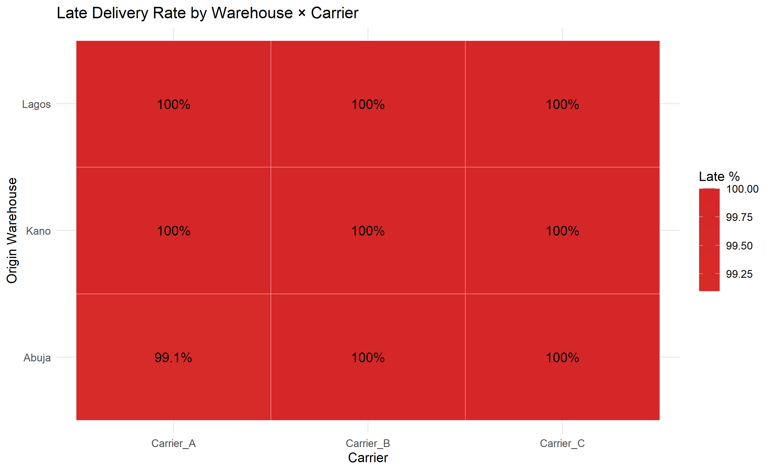
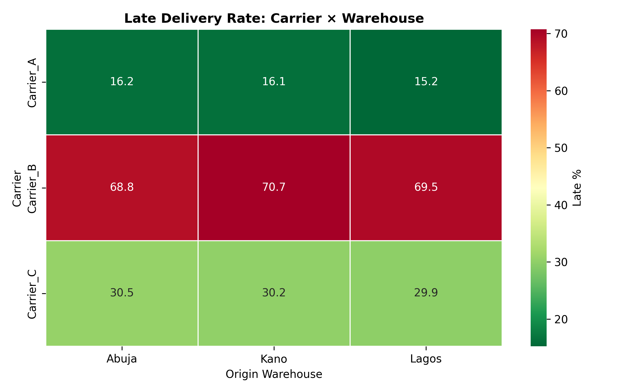
A Pareto analysis often reveals 80/20 patterns: "80% of late deliveries occur on 20% of routes." Targeting these high-impact routes yields disproportionate benefits. A heatmap of late delivery rate by origin warehouse and destination state visualises geographic problem areas.
::: {.panel-tabset}
## R
```{r}
#| label: ch48-eda-late-deliveries
#| message: false
library(tidyverse)
# Use supply_data and order_metrics from previous section
# 1. Pareto: which routes account for most late deliveries?
route_late <- supply_data |>
filter(Delivered_On_Time == 0) |>
group_by(Origin_Warehouse, Destination_State) |>
summarise(late_count = n(), .groups = "drop") |>
arrange(desc(late_count)) |>
mutate(
route = paste(Origin_Warehouse, "→", Destination_State),
cum_pct = cumsum(late_count) / sum(late_count) * 100
)
cat("=== Top 10 Late Delivery Routes (Pareto) ===\n")
print(head(route_late |> select(route, late_count, cum_pct), 10))
# 2. Delay distribution by carrier
carrier_delay <- supply_data |>
mutate(
days_late = pmax(0, as.numeric(Actual_Delivery_Date - Expected_Delivery_Date))
) |>
group_by(Carrier) |>
summarise(
total_shipments = n(),
pct_late = mean(Delivered_On_Time == 0) * 100,
avg_days_late = mean(days_late[days_late > 0], na.rm = TRUE),
max_days_late = max(days_late),
.groups = "drop"
)
cat("\n=== Delay Profile by Carrier ===\n")
print(carrier_delay)
# 3. Late rate by day of week
dow_late <- supply_data |>
mutate(dow = lubridate::wday(Order_Date, label = TRUE)) |>
group_by(dow) |>
summarise(late_rate = mean(Delivered_On_Time == 0) * 100, .groups = "drop")
cat("\n=== Late Rate by Day of Week (Order Date) ===\n")
print(dow_late)
# 4. Visualise: late rate by origin warehouse & carrier
heatmap_oc <- order_metrics |>
group_by(Origin_Warehouse, Carrier) |>
summarise(
late_rate = (1 - mean(OTIF_Order)) * 100,
.groups = "drop"
)
ggplot(heatmap_oc, aes(x = Carrier, y = Origin_Warehouse, fill = late_rate)) +
geom_tile(colour = "white") +
geom_text(aes(label = paste0(round(late_rate, 1), "%")), size = 4) +
scale_fill_gradient2(low = "#2ca02c", mid = "lightyellow", high = "#d62728",
midpoint = 10) +
labs(
title = "Late Delivery Rate by Warehouse × Carrier",
x = "Carrier", y = "Origin Warehouse", fill = "Late %"
) +
theme_minimal()
```
## Python
```{python}
#| label: py-ch48-eda-late-deliveries
import pandas as pd
import numpy as np
import matplotlib.pyplot as plt
import seaborn as sns
# Use supply_data from previous section
# 1. Pareto: routes with most late deliveries
late_df = supply_data[supply_data['Delivered_On_Time'] == 0].copy()
route_late = (
late_df
.groupby(['Origin_Warehouse', 'Destination_State'])
.size().reset_index(name='late_count')
.sort_values('late_count', ascending=False)
)
route_late['route'] = route_late['Origin_Warehouse'] + ' → ' + route_late['Destination_State']
route_late['cum_pct'] = route_late['late_count'].cumsum() / route_late['late_count'].sum() * 100
print("=== Top 10 Late Delivery Routes (Pareto) ===")
print(route_late[['route', 'late_count', 'cum_pct']].head(10).to_string(index=False))
# 2. Delay days by carrier
supply_data['days_late'] = (
(supply_data['Actual_Delivery_Date'] - supply_data['Expected_Delivery_Date'])
.dt.days.clip(lower=0)
)
carrier_delay = supply_data.groupby('Carrier').agg(
total_shipments = ('Delivered_On_Time', 'count'),
pct_late = ('Delivered_On_Time', lambda x: (1 - x.mean()) * 100),
avg_days_late = ('days_late', lambda x: x[x > 0].mean()),
max_days_late = ('days_late', 'max')
).round(2)
print("\n=== Delay Profile by Carrier ===")
print(carrier_delay.to_string())
# 3. Visualise: late rate heatmap (use supply_data which has Origin_Warehouse)
pivot = supply_data.groupby(['Carrier', 'Origin_Warehouse'])['Delivered_On_Time'].mean().unstack()
pivot = 1 - pivot # Convert on-time rate to late rate
fig, ax = plt.subplots(figsize=(8, 5))
sns.heatmap(pivot * 100, annot=True, fmt='.1f', cmap='RdYlGn_r',
linewidths=0.5, cbar_kws={'label': 'Late %'}, ax=ax)
ax.set_title('Late Delivery Rate: Carrier × Warehouse', fontweight='bold')
ax.set_xlabel('Origin Warehouse')
ax.set_ylabel('Carrier')
plt.tight_layout()
plt.show()
```
:::
## Late Delivery Prediction
Once patterns are identified, predictive models anticipate which shipments will be late **before departure**. This enables proactive intervention: expediting, rerouting, or customer communication. Classification models (logistic regression, random forest, XGBoost) predict binary outcome: Will this shipment be delivered late (1) or on time (0)?
Features:
- **Carrier:** Carrier_A vs B vs C have different reliability
- **Route:** Origin warehouse + destination state encode distance and condition
- **Product category:** Certain categories (medicines) require special handling, risking delays
- **Order characteristics:** Large orders may saturate local handling capacity
- **Temporal:** Orders placed on Fridays may defer movement until Monday
- **Carrier load:** If carrier is heavily loaded, delays cascade
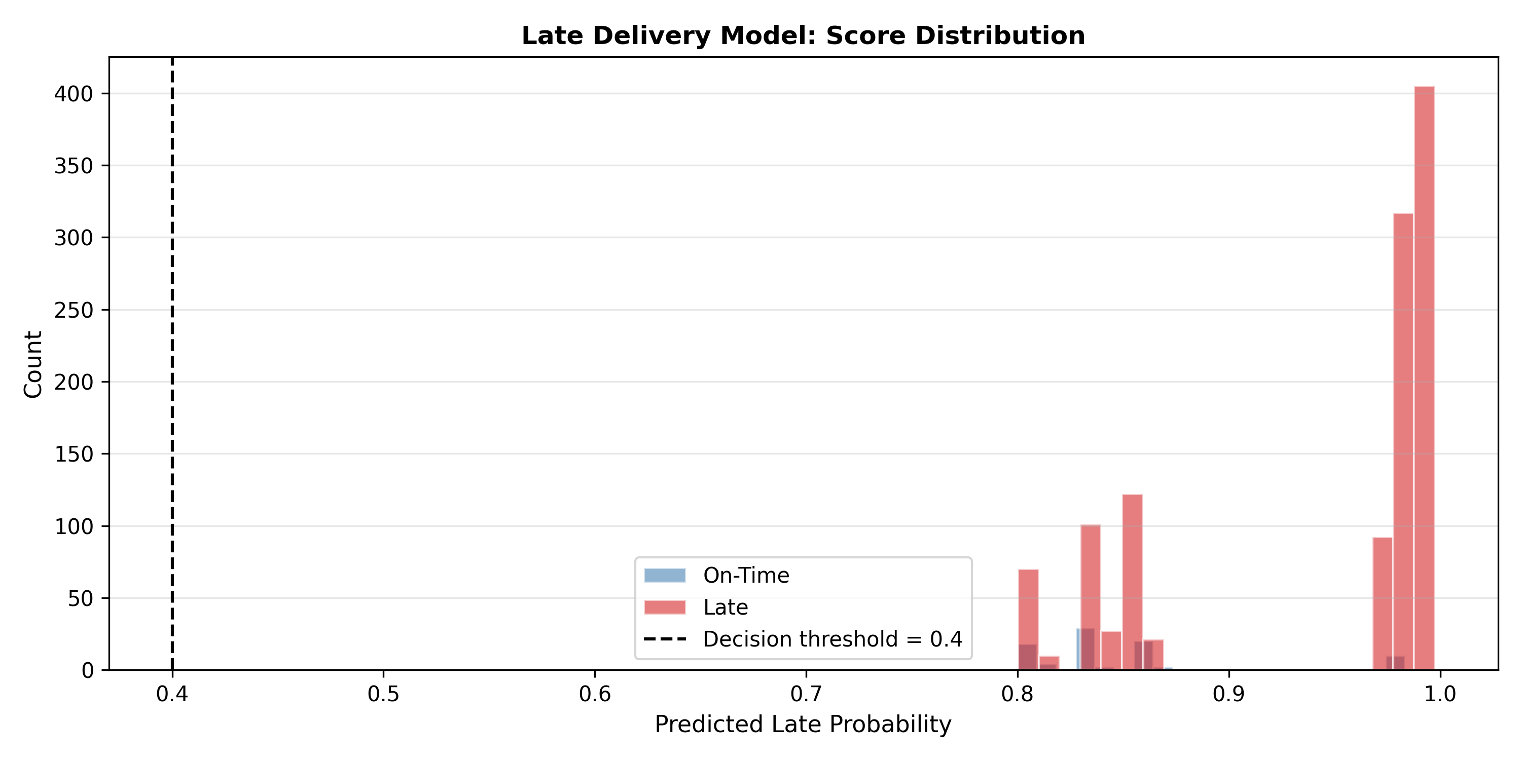
Model evaluation uses classification metrics (precision, recall, F1) and ROI analysis: cost of false positives (expediting a shipment that would arrive on time) vs false negatives (failing to flag a late shipment, incurring customer penalty).
::: {.panel-tabset}
## R
```{r}
#| label: ch48-late-delivery-model
#| message: false
library(tidyverse)
library(pROC)
set.seed(6042)
# Build feature set at order level
model_data <- order_metrics |>
mutate(
carrier_B = as.integer(Carrier == "Carrier_B"),
carrier_C = as.integer(Carrier == "Carrier_C"),
dest_remote = as.integer(Destination_State %in% c("Kano", "Katsina", "Kebbi")),
dest_mid = as.integer(Destination_State %in% c("Ibadan", "Abeokuta", "Ogun")),
is_friday = as.integer(weekdays(Order_Date) == "Friday"),
y = 1L - All_On_Time
)
# Train/test split
train_idx <- sample(1:nrow(model_data), 0.75 * nrow(model_data))
train <- model_data[train_idx, ]
test <- model_data[-train_idx, ]
# Logistic regression
late_model <- glm(
y ~ carrier_B + carrier_C + dest_remote + dest_mid + is_friday,
data = train, family = binomial
)
cat("=== Late Delivery Prediction Model ===\n")
coef_tbl <- summary(late_model)$coefficients |>
as.data.frame() |>
mutate(
OddsRatio = round(exp(Estimate), 3),
Estimate = round(Estimate, 3),
`Pr(>|z|)` = round(`Pr(>|z|)`, 4)
)
print(coef_tbl[, c("Estimate", "OddsRatio", "Pr(>|z|)")])
# Model performance
test <- test |>
mutate(pred_late_prob = predict(late_model, newdata = test, type = "response"))
roc_obj <- roc(test$y, test$pred_late_prob, quiet = TRUE)
cat("\nAUC:", round(auc(roc_obj), 3), "\n")
# Business value: how many late shipments would we flag if we expedite
# those with pred_late_prob > 0.40?
threshold <- 0.40
test <- test |>
mutate(
flagged = pred_late_prob > threshold,
true_late = y == 1
)
tp <- sum(test$flagged & test$true_late)
fp <- sum(test$flagged & !test$true_late)
fn <- sum(!test$flagged & test$true_late)
cat("\n=== Business Value at Threshold", threshold, "===\n")
cat("Late shipments caught early (TP):", tp, "\n")
cat("On-time shipments unnecessarily flagged (FP, expediting cost):", fp, "\n")
cat("Late shipments missed (FN):", fn, "\n")
cat("Recall (late shipments captured):", round(tp / (tp + fn), 3), "\n")
cat("Precision (flagged shipments that were genuinely late):", round(tp / (tp + fp), 3), "\n")
```
## Python
```{python}
#| label: py-ch48-late-delivery-model
import numpy as np
import pandas as pd
import matplotlib.pyplot as plt
from sklearn.linear_model import LogisticRegression
from sklearn.metrics import roc_auc_score, precision_score, recall_score
from sklearn.model_selection import train_test_split

np.random.seed(6042)

# Feature engineering
md = order_metrics.copy()
md['carrier_B']   = (md['Carrier'] == 'Carrier_B').astype(int)
md['carrier_C']   = (md['Carrier'] == 'Carrier_C').astype(int)
md['dest_remote'] = md['Destination_State'].isin(['Kano', 'Katsina', 'Kebbi']).astype(int)
md['dest_mid']    = md['Destination_State'].isin(['Ibadan', 'Abeokuta', 'Ogun']).astype(int)
md['is_friday']   = (md['Order_Date'].dt.dayofweek == 4).astype(int)
md['y']           = 1 - md['Delivered_On_Time']

features = ['carrier_B', 'carrier_C', 'dest_remote', 'dest_mid', 'is_friday']
X = md[features]
y = md['y']

X_train, X_test, y_train, y_test = train_test_split(X, y, test_size=0.25, random_state=6042)

clf = LogisticRegression(max_iter=500)
clf.fit(X_train, y_train)
pred_prob = clf.predict_proba(X_test)[:, 1]
auc = roc_auc_score(y_test, pred_prob)
print("=== Late Delivery Prediction Model ===")
coef_df = pd.DataFrame({
'Feature': features,
'Coef': clf.coef_[0].round(3),
'OddsRatio': np.exp(clf.coef_[0]).round(3)
})
print(coef_df.to_string(index=False))
print(f"\nAUC: {auc:.3f}")
# Business value at threshold 0.40
threshold = 0.40
pred_class = (pred_prob >= threshold).astype(int)
precision = precision_score(y_test, pred_class, zero_division=0)
recall = recall_score(y_test, pred_class, zero_division=0)
tp = int(((pred_class == 1) & (y_test == 1)).sum())
fp = int(((pred_class == 1) & (y_test == 0)).sum())
fn = int(((pred_class == 0) & (y_test == 1)).sum())
print(f"\n=== Business Value at Threshold {threshold} ===")
print(f"Late shipments caught early (TP): {tp}")
print(f"On-time shipments flagged (FP): {fp}")
print(f"Late shipments missed (FN): {fn}")
print(f"Recall (late captured): {recall:.3f}")
print(f"Precision (flags correct): {precision:.3f}")
# Plot predicted probability distribution
fig, ax = plt.subplots(figsize=(10, 5))
ax.hist(pred_prob[y_test == 0], bins=20, alpha=0.6, label='On-Time',
color='steelblue', edgecolor='white')
ax.hist(pred_prob[y_test == 1], bins=20, alpha=0.6, label='Late',
color='#d62728', edgecolor='white')
ax.axvline(threshold, color='black', linestyle='--', linewidth=1.5,
label=f'Decision threshold = {threshold}')
ax.set_xlabel('Predicted Late Probability', fontsize=11)
ax.set_ylabel('Count', fontsize=11)
ax.set_title('Late Delivery Model: Score Distribution', fontweight='bold')
ax.legend()
ax.grid(axis='y', alpha=0.3)
plt.tight_layout()
plt.show()
```
:::
## Supply Chain Risk Analytics
Resilience depends on supplier diversity and network structure. **Concentration risk** measures whether too much supply comes from one vendor. The Herfindahl-Hirschman Index (HHI) quantifies concentration:
$$\text{HHI} = \sum_i (\text{Market Share}_i)^2$$
HHI = 10,000 = complete monopoly (one supplier 100%). HHI = 2,500 (four equal suppliers, each 25%). HHI > 2,500 signals high concentration. In Nigerian pharma, if 60% of supply comes from a single importer/wholesaler, and that importer faces port delays, the entire supply chain stalls.
**Network resilience** also depends on **single points of failure** (nodes whose failure disconnects the network). A warehouse is a single point of failure if it's the only path from manufacturer to a region. Betweenness centrality (from network analysis, Ch. 30) quantifies this: nodes with high betweenness are critical chokepoints.
## Route Optimisation Basics
The **Vehicle Routing Problem (VRP)** is: given a set of locations and vehicles, find routes minimizing travel distance/time while satisfying constraints (vehicle capacity, delivery time windows). VRP is NP-hard (no polynomial-time algorithm), so heuristics are standard.
**Nearest Neighbour Heuristic:** Start at depot, visit nearest unvisited location, repeat until all visited, return to depot. Fast (O(n²)) but suboptimal.
**Clarke-Wright Savings Algorithm:** Iteratively merge routes that save the most distance. More sophisticated, often yields 85–95% of optimal.
For a last-mile example: 30 retail points in Lagos need daily delivery from a central depot. Nearest neighbour builds routes by greedily visiting nearest stops. Clarke-Wright savings (e.g., merging route (depot-A-depot) and (depot-B-depot) into (depot-A-B-depot)) reduces total distance.
## Case Study: Supply Chain Analytics for a West African FMCG Distributor
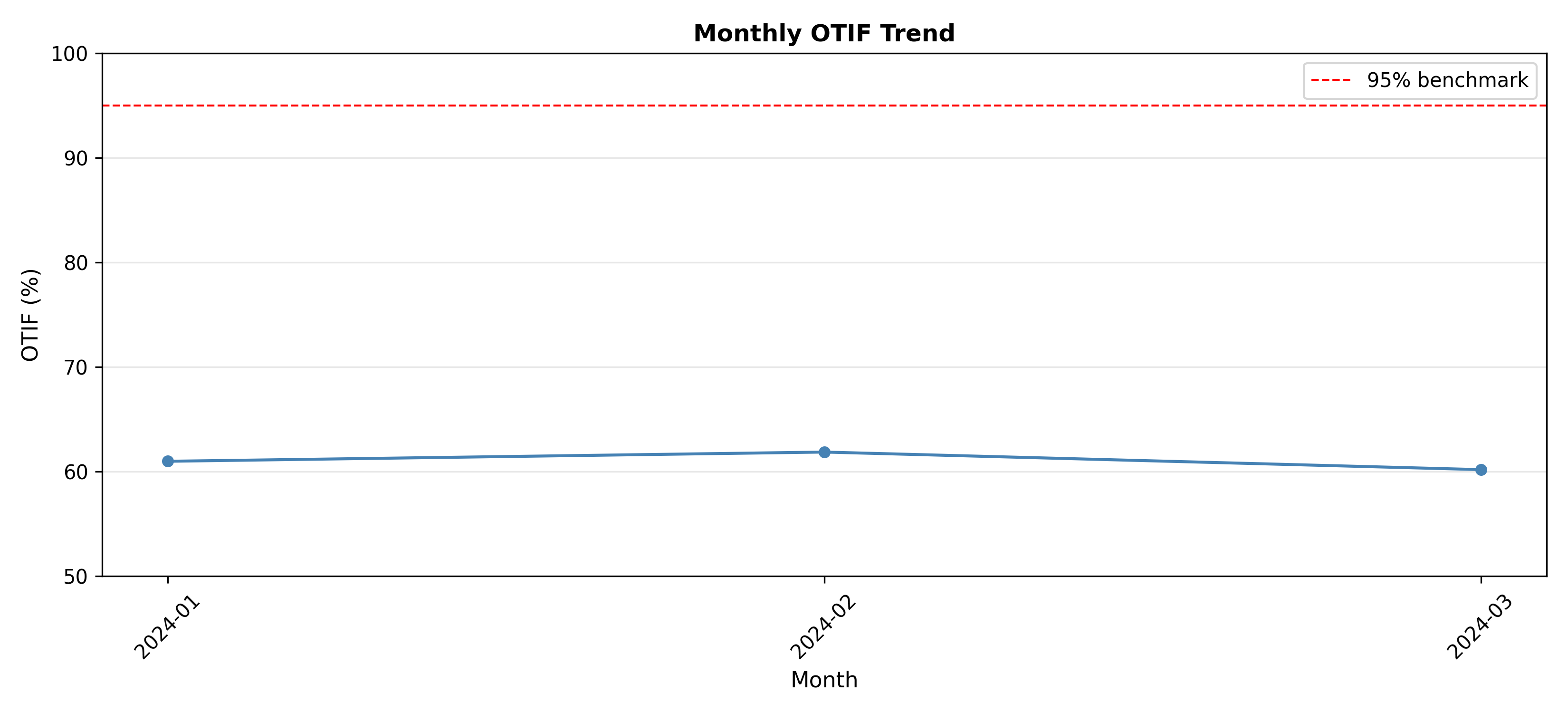
**Background**: A fictional fast-moving consumer goods distributor (beverages, snacks, toiletries) operates three warehouses (Lagos, Abuja, Kano) and services 8 states through 3 carriers. OTIF currently runs at 88%, below the industry benchmark of 95%. Stockouts cost the company approximately ₦180 million per year. Management wants to: (a) identify the primary causes of missed OTIF, (b) predict which future shipments will be late, and (c) design an improvement program.
**Analytical workflow** (using the 50,000 order-line dataset generated earlier):
::: {.panel-tabset}
## R
```{r}
#| label: ch48-case-study
#| message: false
library(tidyverse)
# Step 1: Root-cause ranking
cat("=== Step 1: Root-Cause Analysis ===\n")
cause_decomp <- order_metrics |>
summarise(
pct_late_delivery = (1 - mean(All_On_Time)) * 100,
pct_incomplete_fill = (1 - mean(All_Complete)) * 100,
pct_otif_failure = (1 - mean(OTIF_Order)) * 100
)
cat("Failure decomposition:\n")
cat(" - Orders late to destination: ", round(cause_decomp$pct_late_delivery, 1), "%\n")
cat(" - Orders with incomplete fill: ", round(cause_decomp$pct_incomplete_fill, 1), "%\n")
cat(" - OTIF failures (either late or short):", round(cause_decomp$pct_otif_failure, 1), "%\n")
# Step 2: Carrier scorecard
cat("\n=== Step 2: Carrier Performance Scorecard ===\n")
carrier_scorecard <- order_metrics |>
group_by(Carrier) |>
summarise(
orders = n(),
otif_pct = mean(OTIF_Order) * 100,
otd_pct = mean(All_On_Time) * 100,
fill_pct = mean(All_Complete) * 100,
.groups = "drop"
) |>
arrange(otif_pct)
print(carrier_scorecard |>
mutate(across(c(otif_pct, otd_pct, fill_pct), ~ round(., 1))))
# Step 3: State risk tier
cat("\n=== Step 3: State Risk Tiers ===\n")
state_tier <- order_metrics |>
group_by(Destination_State) |>
summarise(otif = mean(OTIF_Order) * 100, .groups = "drop") |>
mutate(
risk_tier = case_when(
otif >= 95 ~ "Green (On Target)",
otif >= 88 ~ "Amber (At Risk)",
TRUE ~ "Red (Critical)"
)
)
print(state_tier)
# Step 4: Improvement scenario
cat("\n=== Step 4: Improvement Scenario ===\n")
cat("Current OTIF:", round(mean(order_metrics$OTIF_Order) * 100, 1), "%\n")
cat("If Carrier_B delays improved to Carrier_A standard:\n")
# Carrier_B's contribution to total failures
carrier_b_failures <- order_metrics |>
filter(Carrier == "Carrier_B", OTIF_Order == 0) |> nrow()
total_orders <- nrow(order_metrics)
improvement <- carrier_b_failures * 0.50 / total_orders * 100
cat(" → Estimated OTIF improvement:", round(improvement, 1), "percentage points\n")
cat(" → New OTIF target:", round(mean(order_metrics$OTIF_Order) * 100 + improvement, 1), "%\n")
cat("\nStrategic recommendations:\n")
cat("1. Review Carrier_B contract: SLA enforcement for delay penalties\n")
cat("2. Route high-value orders through Carrier_A for remote states\n")
cat("3. Increase safety stock for Medicines (lowest fill rate product category)\n")
cat("4. Deploy late-delivery prediction model to trigger pre-emptive re-routing\n")
# Visualise: OTIF over time (simulated monthly trend)
monthly_otif <- supply_data |>
mutate(month = lubridate::floor_date(Order_Date, "month")) |>
group_by(month) |>
summarise(otif_rate = mean(Delivered_On_Time) * 100, .groups = "drop")
ggplot(monthly_otif, aes(x = month, y = otif_rate)) +
geom_line(colour = "steelblue", linewidth = 1.2) +
geom_point(colour = "steelblue", size = 2.5) +
geom_hline(yintercept = 95, linetype = "dashed", colour = "red",
linewidth = 0.8) +
labs(
title = "Monthly OTIF Trend",
x = NULL, y = "OTIF (%)",
subtitle = "Red dashed line = 95% industry benchmark"
) +
ylim(50, 100) +
theme_minimal()
```
## Python
```{python}
#| label: py-ch48-case-study
import pandas as pd
import numpy as np
import matplotlib.pyplot as plt
# Root-cause analysis
print("=== Step 1: Root-Cause Analysis ===")
pct_late = (1 - order_metrics['Delivered_On_Time'].mean()) * 100
pct_inc = (1 - order_metrics['All_Complete'].mean()) * 100
pct_otif = (1 - order_metrics['OTIF'].mean()) * 100
print(f" Late delivery failures: {pct_late:.1f}%")
print(f" Incomplete fill failures: {pct_inc:.1f}%")
print(f" OTIF failures (any): {pct_otif:.1f}%")
# Carrier scorecard
print("\n=== Step 2: Carrier Scorecard ===")
scorecard = order_metrics.groupby('Carrier').agg(
orders = ('OTIF', 'count'),
otif_pct = ('OTIF', lambda x: x.mean() * 100),
otd_pct = ('Delivered_On_Time', lambda x: x.mean() * 100),
fill_pct = ('All_Complete', lambda x: x.mean() * 100)
).round(1).sort_values('otif_pct')
print(scorecard.to_string())
# State risk tiers
print("\n=== Step 3: State Risk Tiers ===")
state_tier = order_metrics.groupby('Destination_State').agg(
otif = ('OTIF', lambda x: x.mean() * 100)
).round(1)
state_tier['risk_tier'] = np.where(
state_tier['otif'] >= 95, 'Green (On Target)',
np.where(state_tier['otif'] >= 88, 'Amber (At Risk)', 'Red (Critical)')
)
print(state_tier.sort_values('otif').to_string())
# Monthly OTIF trend
supply_data['month'] = supply_data['Order_Date'].dt.to_period('M')
monthly = supply_data.groupby('month')['Delivered_On_Time'].mean() * 100
fig, ax = plt.subplots(figsize=(11, 5))
ax.plot(monthly.index.astype(str), monthly.values, marker='o',
linewidth=1.5, markersize=5, color='steelblue')
ax.axhline(95, linestyle='--', color='red', linewidth=1, label='95% benchmark')
ax.set_xlabel('Month', fontsize=11)
ax.set_ylabel('OTIF (%)', fontsize=11)
ax.set_title('Monthly OTIF Trend', fontweight='bold')
ax.legend()
ax.tick_params(axis='x', rotation=45)
ax.set_ylim(50, 100)
ax.grid(axis='y', alpha=0.3)
plt.tight_layout()
plt.show()
```
:::
::: {.exercises}
#### Chapter 48 Exercises
1. **OTIF Decomposition**: Using the supply chain dataset, calculate the joint probability of on-time AND in-full delivery. Does $P(\text{OTIF}) = P(\text{On-Time}) \times P(\text{In-Full})$? What does a deviation tell you?
2. **Carrier Comparison**: Perform a chi-square test comparing on-time delivery rates across the three carriers. Report the test statistic and p-value. Which pairwise differences are statistically significant?
3. **Predictive Model Extension**: Add a "high value order" indicator (total order value above the 75th percentile) to the late-delivery prediction model. Does it improve AUC? Interpret the odds ratio.
4. **Safety Stock Calculation**: For a product with weekly demand $\mu = 500$ units and standard deviation $\sigma = 80$ units, and a lead time of 7 days, calculate the safety stock needed for a 95% service level. (Hint: safety stock = $z \times \sigma \times \sqrt{L}$, where $z = 1.645$ for 95%.)
5. **Route Optimisation**: Simulate the nearest-neighbour VRP heuristic for 15 retail delivery points in a city. Generate random (x, y) coordinates and compute the total tour distance. Compare to the optimal tour found by brute force (feasible for ≤ 10 points).
6. **Network Resilience**: Build a supply network graph with 5 warehouses and 12 routes. Compute betweenness centrality for each warehouse. Remove the highest-centrality node and measure how many routes become disconnected. What does this imply for supply chain design?
:::
---
## Further Reading
- **Bowersox, Closs & Cooper (2013). "Supply Chain Logistics Management"**
- **OpenRouteService:** Free VRP solver at https://openrouteservice.org/
- **PySpark: Distributed logistics modelling for large networks**
---
## Chapter 48 Appendix: Mathematical Derivations
### A48.1 Bullwhip Effect Mathematical Model
Let $D_t$ = demand in period $t$, $O_t$ = orders placed. Assume linear demand forecast: $F_t = D_t + \alpha(D_t - D_{t-1})$, where $\alpha$ is forecast adjustment coefficient. Orders: $O_t = F_t + S_t$ (forecast + safety stock adjustment).
Substituting:
$$O_t = D_t + \alpha(D_t - D_{t-1}) + S_t$$
If $D_t$ follows an AR(1) process $D_t = \rho D_{t-1} + \epsilon_t$, then variance of $O_t$ is:
$$\text{Var}(O_t) = \left[1 + \alpha(\alpha + 2)\right] \text{Var}(D_t) + (1 + \alpha)^2 \text{Var}(S_t)$$
The multiplier $[1 + \alpha(\alpha + 2)]$ > 1 (for $\alpha > 0$) shows order variance amplification.
### A48.2 OTIF Decomposition
OTIF combines timeliness and completeness:
$$\text{OTIF} = P(\text{On Time}) \times P(\text{In Full | On Time})$$
If on-time and in-full are independent:
$$\text{OTIF} \approx P(\text{On Time}) \times P(\text{In Full})$$
Typically, $P(\text{On Time}) = 0.96$ and $P(\text{In Full}) = 0.94$, yielding OTIF ≈ 0.90 (90%).
### A48.3 HHI for Supplier Concentration
$$\text{HHI} = \sum_{i=1}^{n} S_i^2$$
where $S_i$ is supplier $i$'s share of total supply volume. Maximum = 10,000 (monopoly), minimum = 10,000/n (n equal suppliers).
### A48.4 Clarke-Wright Savings Algorithm
For each pair of nodes $i$ and $j$, the savings from merging two routes is:
$$s_{ij} = d_{0i} + d_{0j} - d_{ij}$$
where $d_{0i}$ is distance from depot to node $i$. Sort savings in descending order and greedily merge routes, respecting vehicle capacity.
### A48.5 Betweenness Centrality in Supply Networks
$$C_B(v) = \sum_{s \neq v \neq t} \frac{\sigma_{st}(v)}{\sigma_{st}}$$
where $\sigma_{st}(v)$ is the number of shortest paths from $s$ to $t$ that pass through $v$, and $\sigma_{st}$ is the total number of shortest paths. High $C_B(v)$ indicates $v$ is a critical intermediary.
---
**End of Chapter 48**