---
title: "Marketing Mix Analytics"
author: "Bongo Adi"
---
```{python}
#| label: python-setup-45-marketing-mix-analytics
#| include: false
import numpy as np
import pandas as pd
import matplotlib.pyplot as plt
import seaborn as sns
from scipy import optimize
from sklearn.linear_model import Ridge, LinearRegression
from scipy import stats
from scipy.stats import norm
from scipy.optimize import minimize, LinearConstraint, Bounds
```
::: {.callout-note icon="false"}
## 📋 Learning Objectives
- Understand the principles and applications of Marketing Mix Modelling (MMM) in decomposing sales by marketing channel
- Master the Adstock transformation and saturation curves for realistic media response modelling
- Build and interpret MMM regression models with control variables and seasonal adjustment
- Apply Bayesian methods to quantify uncertainty in channel attribution
- Decompose revenue contributions and calculate marginal ROI by channel
- Optimise marketing budget allocation across channels to maximise total revenue
- Implement MMM workflows in both R and Python with Nigerian consumer goods data
:::
## What Is Marketing Mix Modelling?
Marketing Mix Modelling (MMM) is a statistical technique that decomposes total sales or revenue into the contributions from each marketing channel—television, radio, digital, outdoor, influencers, and more. In the post-cookie era, where third-party audience data has become scarce and conversion tracking fragmented, MMM provides marketers with an aggregate-level view of channel effectiveness without requiring individual-level tracking. The core business question is deceptively simple: "How much of our revenue came from TV versus radio versus digital versus out-of-home advertising?"
In the Nigerian context, this question becomes particularly nuanced. Nigerian brands operate across extraordinarily diverse media ecosystems. Television remains a mass reach medium—national networks like NTA, Channels Television, AIT, and numerous regional Hausa-language stations (BBC Hausa, Voice of Nigeria) still command significant audiences, particularly in Northern and rural markets. Radio, often dismissed in developed markets, remains a primary medium in Nigeria, with heavy listenership during morning drive times and afternoon commutes. Traditional outdoor billboards along major corridors—the Lagos-Ibadan Expressway, the Abeokuta-Ibadan road, and routes into Abuja—reach commuters and travelers daily. Digital channels (Facebook, Instagram, Google Search, TikTok) have exploded in urban centres and are increasingly accessible via mobile-only consumers. Influencer marketing, from mega-influencers with millions of followers to micro-influencers with hyper-local reach, has become a significant spend category for consumer goods brands targeting youth demographics.
Why MMM matters more than ever is rooted in this fragmentation and the erosion of deterministic attribution. A decade ago, advertisers could often trace a customer's path: click a Facebook ad, land on a website, make a purchase, and credit Facebook with the conversion. Today, the customer journey is far more opaque. A consumer might see a TV commercial on DStv or StarTimes, remember the brand vaguely, search for it on Google days later, see a retargeting ad on Instagram, and finally purchase offline at a Shoprite or Naira box corner shop. Which channel deserves credit? MMM sidesteps this attribution problem by using statistical modelling to estimate how much each channel contributed to aggregate sales, even without individual-level conversion data. It answers the question with confidence intervals, acknowledging the inherent uncertainty in attribution estimation.
## The Adstock Transformation
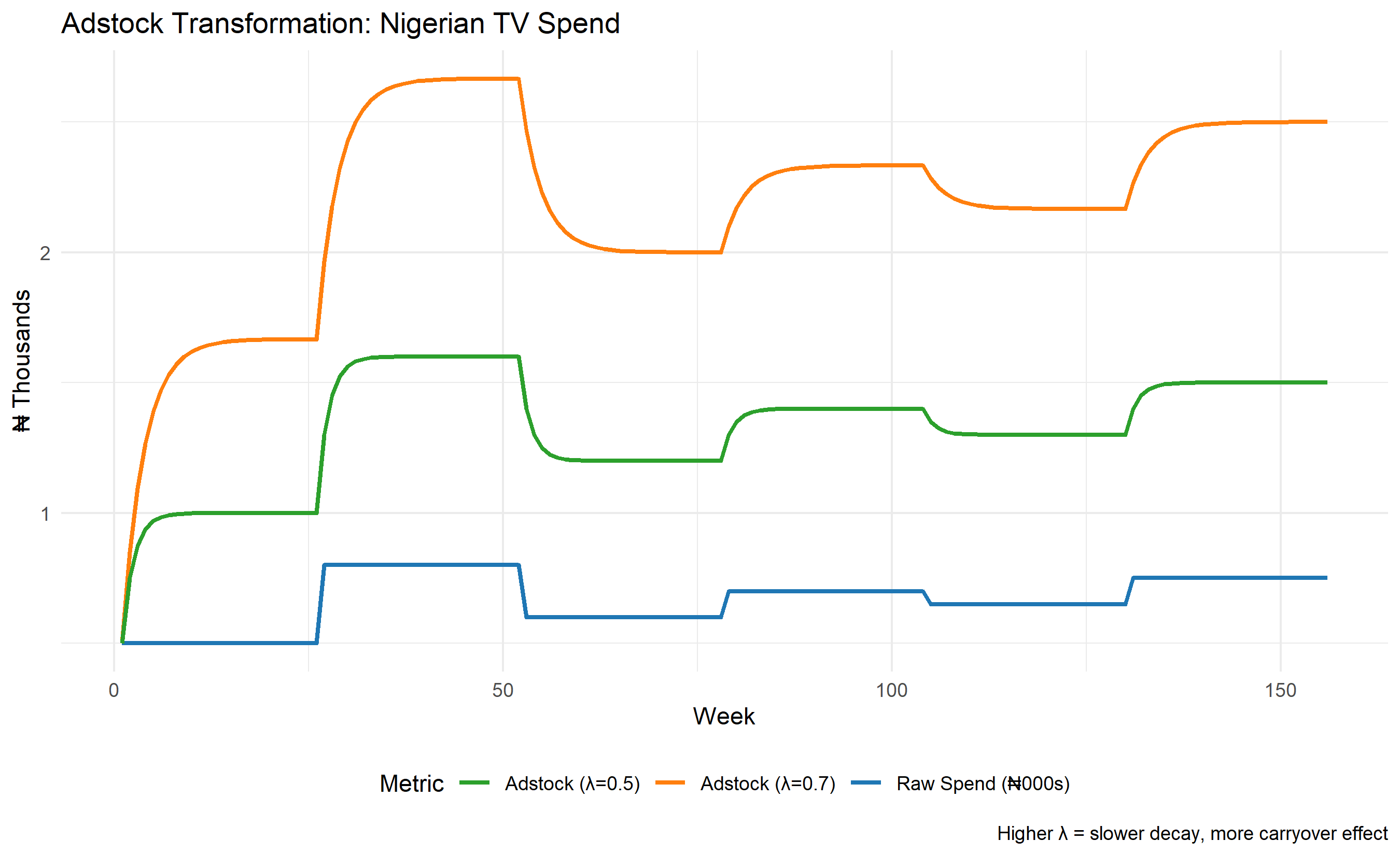
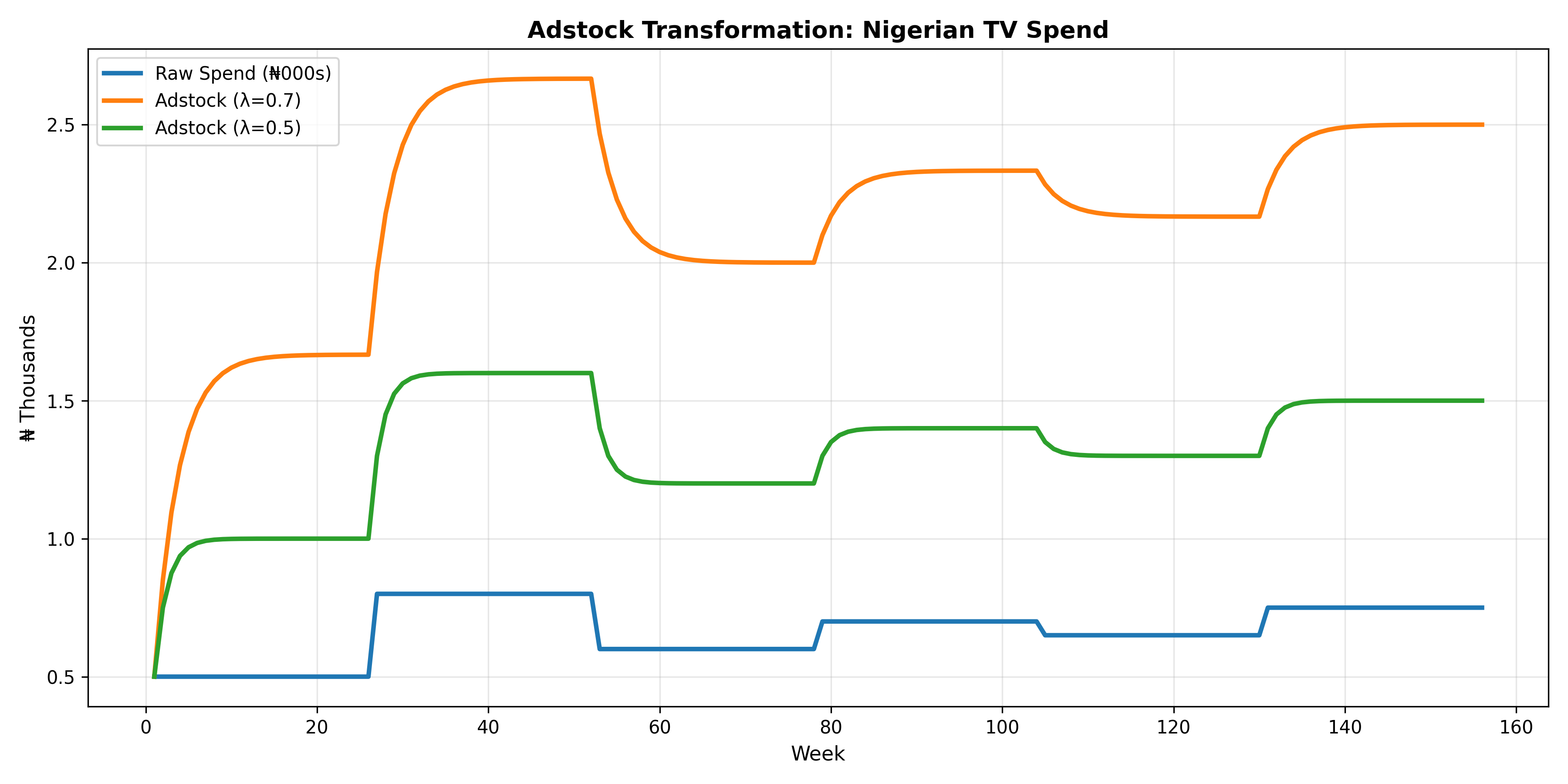
Advertising does not produce instantaneous sales. A television commercial aired on Monday does not cause a purchase solely on Monday; rather, some of its effect decays over subsequent days and weeks. This carryover effect—the delayed and diminishing impact of advertising—is fundamental to realistic media modelling. The Adstock transformation is a mathematical tool that converts raw media spend into a "stock" of advertising goodwill that decays geometrically over time.
The core Adstock recurrence relation is:
$$\text{Adstock}_t = \text{Spend}_t + \lambda \times \text{Adstock}_{t-1}$$
where $\text{Spend}_t$ is the media spend in period $t$ (say, a week), $\lambda$ is the decay rate (typically between 0 and 1), and $\text{Adstock}_{t-1}$ is the carryover from the previous period. When $\lambda = 0$, there is no carryover—the effect is instantaneous. When $\lambda = 0.5$, 50% of the advertising stock persists from one period to the next. As $\lambda$ approaches 1, the advertising effect becomes quasi-permanent, which is unrealistic for most categories. A practical decay rate of $\lambda = 0.7$ implies a half-life (the time for the effect to decay to 50% of its peak) of about 3 weeks; this can be calculated as $\text{half-life} = \log(0.5) / \log(\lambda)$.
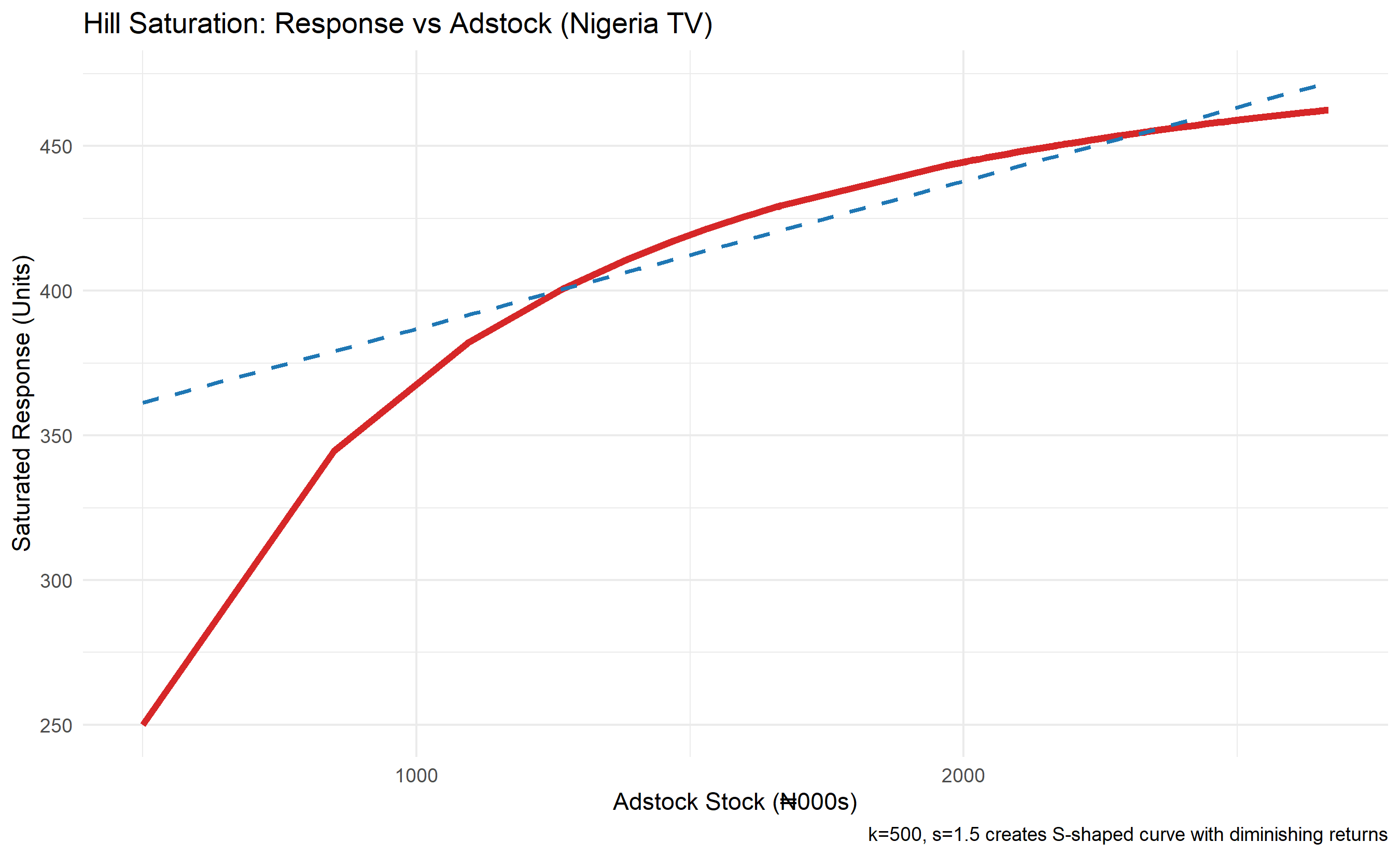
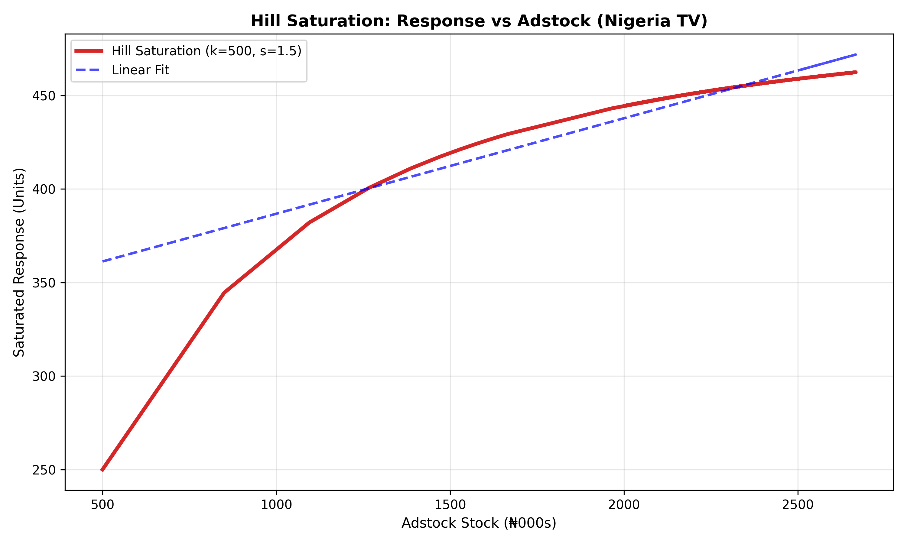
Beyond carryover lies saturation: the observation that each additional dollar of advertising generates fewer additional sales. This is the principle of diminishing returns. A brand with zero awareness must spend heavily on reach to build initial awareness, but once awareness plateaus at, say, 80%, additional spend achieves less relative gain. The Hill saturation function captures this curvature:
$$\text{Response}_t = \frac{k \times \text{Adstock}_t^s}{k^s + \text{Adstock}_t^s}$$
where $k$ is the half-saturation point (the Adstock level at which response reaches 50% of maximum), and $s$ is the shape parameter. When $s = 1$, the function is linear (no saturation). When $s > 1$, the curve exhibits S-shaped diminishing returns characteristic of most real advertising response.
The Adstock transformation matters tremendously in Nigerian marketing contexts because traditional media (TV and radio) have inherent carryover effects tied to viewer and listener routines. A television commercial broadcast on prime time (8–10 PM on weekdays) reaches a concentrated audience, but the brand recall persists for days, especially for established brands. Radio spots, often repeated multiple times across a week, build message frequency and top-of-mind awareness through repetition and decay dynamics. Digital channels, by contrast, often show shorter lags and faster decay; a Facebook ad is seen, forgotten, and superseded by new content within hours unless reinforced. Outdoor billboards operate on a different temporal rhythm—a driver passes a billboard once or twice daily, and the cumulative exposure builds mental associations over weeks. Failing to model these differences would lead to systematic overestimation of digital effectiveness and underestimation of traditional media's true contribution.
::: {.callout-note icon="false"}
## 📘 Theory: Adstock and Saturation in Media Response
The Adstock transformation converts media spend into a lagged stock that decays geometrically. This stock then saturates—additional units of stock produce diminishing returns. Together, Adstock and saturation form the foundation of realistic media response curves. The Adstock formula can also be written as an infinite sum of decaying past spend: $\text{Adstock}_t = \sum_{i=0}^{\infty} \lambda^i \times \text{Spend}_{t-i}$. The Hill saturation function is one of several choices; alternatives include the logistic curve $\frac{1}{1 + e^{-s(\text{Adstock}_t - k)}}$ and the Michaelis-Menten function. The choice of saturation functional form can significantly affect estimated ROI, and sensitivity analysis across functional forms is recommended best practice.
:::
::: {.callout-tip icon="false"}
## 🔑 Key Formulas
**Adstock Recurrence:**
$$\text{Adstock}_t = \text{Spend}_t + \lambda \times \text{Adstock}_{t-1}$$
**Half-Life Decay:**
$$\text{Half-life} = \frac{\log(0.5)}{\log(\lambda)}$$
**Hill Saturation Function:**
$$\text{Response}_t = \frac{k \times \text{Adstock}_t^s}{k^s + \text{Adstock}_t^s}$$
:::
::: {.panel-tabset}
## R
```{r}
#| label: ch45-adstock-saturation
#| message: false
#| warning: false
library(tidyverse)
library(ggplot2)

# Set seed for reproducibility
set.seed(6247)

# Simulate synthetic Nigerian TV spend data: 156 weeks (3 years)
weeks <- 156
tv_spend <- c(
  rep(500, 26),    # Year 1, Q1-Q2: ₦500k/week
  rep(800, 26),    # Year 1, Q3-Q4: ₦800k/week (boost)
  rep(600, 26),    # Year 2, Q1-Q2: ₦600k/week
  rep(700, 26),    # Year 2, Q3-Q4: ₦700k/week
  rep(650, 26),    # Year 3, Q1-Q2: ₦650k/week
  rep(750, 26)     # Year 3, Q3-Q4: ₦750k/week
)

# Compute Adstock with decay rate λ = 0.7
compute_adstock <- function(spend, lambda) {
  adstock <- numeric(length(spend))
  adstock[1] <- spend[1]
  for (t in 2:length(spend)) {
    adstock[t] <- spend[t] + lambda * adstock[t - 1]
  }
  return(adstock)
}

# Compute for λ = 0.7 and λ = 0.5
adstock_0.7 <- compute_adstock(tv_spend, lambda = 0.7)
adstock_0.5 <- compute_adstock(tv_spend, lambda = 0.5)

# Hill saturation function
hill_saturation <- function(adstock, k, s) {
  (k * adstock^s) / (k^s + adstock^s)
}

# Apply saturation (k = 500, s = 1.5 for moderate S-curve)
response_saturated <- hill_saturation(adstock_0.7, k = 500, s = 1.5)

# Create data frame for visualisation
df <- tibble(
  Week = 1:weeks,
  TV_Spend = tv_spend,
  Adstock_0.7 = adstock_0.7,
  Adstock_0.5 = adstock_0.5,
  Saturated_Response = response_saturated
)

# Plot 1: Adstock transformation
p1 <- ggplot(df, aes(x = Week)) +
  geom_line(aes(y = TV_Spend / 1000, colour = "Raw Spend (₦000s)"), linewidth = 1) +
  geom_line(aes(y = Adstock_0.7 / 1000, colour = "Adstock (λ=0.7)"), linewidth = 1) +
  geom_line(aes(y = Adstock_0.5 / 1000, colour = "Adstock (λ=0.5)"), linewidth = 1) +
  scale_colour_manual(
    values = c("Raw Spend (₦000s)" = "#1f77b4",
               "Adstock (λ=0.7)" = "#ff7f0e",
               "Adstock (λ=0.5)" = "#2ca02c")
  ) +
  labs(
    title = "Adstock Transformation: Nigerian TV Spend",
    x = "Week",
    y = "₦ Thousands",
    colour = "Metric",
    caption = "Higher λ = slower decay, more carryover effect"
  ) +
  theme_minimal() +
  theme(legend.position = "bottom")

print(p1)
# Plot 2: Saturation curve
p2 <- ggplot(df, aes(x = Adstock_0.7)) +
  geom_line(aes(y = Saturated_Response), colour = "#d62728", linewidth = 1.5) +
  geom_smooth(aes(y = Saturated_Response), method = "lm", se = FALSE,
              linetype = "dashed", colour = "#1f77b4", label = "Linear fit") +
  labs(
    title = "Hill Saturation: Response vs Adstock (Nigeria TV)",
    x = "Adstock Stock (₦000s)",
    y = "Saturated Response (Units)",
    caption = "k=500, s=1.5 creates S-shaped curve with diminishing returns"
  ) +
  theme_minimal()

print(p2)
# Calculate and print half-life for λ = 0.7
half_life_0.7 <- log(0.5) / log(0.7)
cat("\n--- Adstock Decay Analysis ---\n")
cat("Half-life (λ = 0.7):", round(half_life_0.7, 2), "weeks\n")
cat("After 4 weeks:", round(0.7^4 * 100, 2), "% of peak effect remains\n")
cat("After 8 weeks:", round(0.7^8 * 100, 2), "% of peak effect remains\n")
# Saturation analysis at different adstock levels
adstock_levels <- c(250, 500, 750, 1000, 1500)
saturation_df <- tibble(
Adstock_Level = adstock_levels,
Saturated_Response = hill_saturation(adstock_levels, k = 500, s = 1.5),
Marginal_Response = c(
NA,
(hill_saturation(500, 500, 1.5) - hill_saturation(250, 500, 1.5)) / (500 - 250),
(hill_saturation(750, 500, 1.5) - hill_saturation(500, 500, 1.5)) / (750 - 500),
(hill_saturation(1000, 500, 1.5) - hill_saturation(750, 500, 1.5)) / (1000 - 750),
(hill_saturation(1500, 500, 1.5) - hill_saturation(1000, 500, 1.5)) / (1500 - 1000)
)
)
cat("\n--- Saturation Effect Analysis ---\n")
print(saturation_df)
```
## Python
```{python}
#| label: py-ch45-adstock-saturation
import numpy as np
import pandas as pd
import matplotlib.pyplot as plt
from scipy import optimize

# Set seed for reproducibility
np.random.seed(6247)

# Simulate synthetic Nigerian TV spend: 156 weeks (3 years)
weeks = 156
tv_spend = np.concatenate([
    np.repeat(500, 26),    # Year 1, Q1-Q2: ₦500k/week
    np.repeat(800, 26),    # Year 1, Q3-Q4: ₦800k/week
    np.repeat(600, 26),    # Year 2, Q1-Q2: ₦600k/week
    np.repeat(700, 26),    # Year 2, Q3-Q4: ₦700k/week
    np.repeat(650, 26),    # Year 3, Q1-Q2: ₦650k/week
    np.repeat(750, 26)     # Year 3, Q3-Q4: ₦750k/week
])

def compute_adstock(spend, lambda_param):
    """Compute Adstock using recurrence relation."""
    adstock = np.zeros_like(spend, dtype=float)
    adstock[0] = spend[0]
    for t in range(1, len(spend)):
        adstock[t] = spend[t] + lambda_param * adstock[t - 1]
    return adstock

def hill_saturation(adstock, k, s):
    """Apply Hill saturation function."""
    return (k * adstock ** s) / (k ** s + adstock ** s)

# Compute Adstocks
adstock_0_7 = compute_adstock(tv_spend, 0.7)
adstock_0_5 = compute_adstock(tv_spend, 0.5)

# Apply saturation (k=500, s=1.5)
saturated_response = hill_saturation(adstock_0_7, k=500, s=1.5)

# Create DataFrame
df = pd.DataFrame({
    'Week': np.arange(1, weeks + 1),
    'TV_Spend': tv_spend,
    'Adstock_0_7': adstock_0_7,
    'Adstock_0_5': adstock_0_5,
    'Saturated_Response': saturated_response
})

# Plot 1: Adstock transformation
fig, ax = plt.subplots(figsize=(12, 6))
ax.plot(df['Week'], df['TV_Spend'] / 1000, label='Raw Spend (₦000s)',
        linewidth=2.5, color='#1f77b4')
ax.plot(df['Week'], df['Adstock_0_7'] / 1000, label='Adstock (λ=0.7)',
        linewidth=2.5, color='#ff7f0e')
ax.plot(df['Week'], df['Adstock_0_5'] / 1000, label='Adstock (λ=0.5)',
        linewidth=2.5, color='#2ca02c')
ax.set_xlabel('Week', fontsize=11)
ax.set_ylabel('₦ Thousands', fontsize=11)
ax.set_title('Adstock Transformation: Nigerian TV Spend', fontsize=13, fontweight='bold')
ax.legend(loc='upper left')
ax.grid(alpha=0.3)
plt.tight_layout()
plt.show()
# Plot 2: Saturation curve
fig, ax = plt.subplots(figsize=(10, 6))
ax.plot(df['Adstock_0_7'], df['Saturated_Response'], linewidth=3,
        color='#d62728', label='Hill Saturation (k=500, s=1.5)')
# Linear fit for comparison
z = np.polyfit(df['Adstock_0_7'], df['Saturated_Response'], 1)
p = np.poly1d(z)
ax.plot(df['Adstock_0_7'], p(df['Adstock_0_7']), 'b--', alpha=0.7,
        linewidth=2, label='Linear Fit')
ax.set_xlabel('Adstock Stock (₦000s)', fontsize=11)
ax.set_ylabel('Saturated Response (Units)', fontsize=11)
ax.set_title('Hill Saturation: Response vs Adstock (Nigeria TV)',
             fontsize=13, fontweight='bold')
ax.legend()
ax.grid(alpha=0.3)
plt.tight_layout()
plt.show()
# Analysis
half_life_0_7 = np.log(0.5) / np.log(0.7)
print("\n--- Adstock Decay Analysis ---")
print(f"Half-life (λ = 0.7): {half_life_0_7:.2f} weeks")
print(f"After 4 weeks: {0.7**4 * 100:.2f}% of peak effect remains")
print(f"After 8 weeks: {0.7**8 * 100:.2f}% of peak effect remains")
# Saturation analysis
adstock_levels = np.array([250, 500, 750, 1000, 1500])
saturated_responses = hill_saturation(adstock_levels, k=500, s=1.5)
saturation_table = pd.DataFrame({
'Adstock_Level': adstock_levels,
'Saturated_Response': saturated_responses,
'Marginal_Response': np.diff(saturated_responses, prepend=np.nan) / np.diff(
np.concatenate([[0], adstock_levels[:-1]]), prepend=np.nan)
})
print("\n--- Saturation Effect Analysis ---")
print(saturation_table.to_string(index=False))
```
:::
## The MMM Regression Model
The MMM regression model decomposes observed sales into their constituent drivers. The core specification is:
$$\text{Sales}_t = \beta_0 + \sum_{c} \beta_c \times \text{Adstock}_{c,t} + \sum_{x} \gamma_x \times \text{Control}_{x,t} + \epsilon_t$$
where $\text{Sales}_t$ is total sales in week $t$, $\beta_0$ is the base sales intercept (the level of sales with zero marketing and no external effects), $\beta_c$ is the marginal revenue per ₦1 of Adstocked spend on channel $c$, and $\gamma_x$ are coefficients on control variables. Control variables are crucial: they account for confounders that might otherwise distort channel estimates. In Nigerian FMCG analysis, typical controls include promotional intensity (fraction of sales on promotion), price changes, competitor activity proxies, seasonality dummies or harmonic terms, macroeconomic controls (quarterly GDP growth, FX rates), religious and cultural calendar effects (Ramadan, Christmas periods when consumption patterns shift dramatically), and supply-side shocks (port congestion, fuel scarcity).
Estimating this model by ordinary least squares (OLS) is computationally simple but suffers from multicollinearity—marketing channels are often correlated in spend patterns (e.g., brands increase all channels in Q4). Ridge regression or regularised regression methods add a penalty term $\lambda \sum \beta_c^2$ to reduce overfitting and stabilise estimates. The interpretability of $\beta_c$ is critical: if TV Adstock has coefficient ₦2.50, this means each ₦1 of Adstocked TV spend increments sales by ₦2.50, a 150% return on that spend (or 2.5x ROI).
Building an MMM model in practice requires careful preprocessing. Adstock parameters (decay rates) for each channel must be either specified a priori based on industry knowledge or searched via grid search to find the values that maximise model fit. Seasonality must be controlled—Nigerian demand for soft drinks spikes in hot months (March–May), ice cream consumption follows similar patterns, while certain FMCG categories (rice, beans) see surges before Christmas. Price elasticity is a control variable that allows the model to distinguish price-driven demand changes from marketing-driven ones. Once the model is fit, residual diagnostics (autocorrelation, heteroscedasticity) must be checked; if serial correlation is present, Newey-West standard errors should be used.
::: {.callout-note icon="false"}
## 📘 Theory: MMM Regression Specification
The MMM regression combines Adstocked channel variables with control variables to decompose sales. The key assumption is that, conditional on controls, the Adstocked channels are exogenous (marketing spend shocks are not driven by unobserved demand shocks). This assumption is often violated in practice—managers increase spend in response to market opportunities—leading to endogeneity bias. Instrumental variable (IV) approaches using historical spend levels or predetermined constraints can mitigate this. The intercept $\beta_0$ represents baseline sales; dividing total sales by $\beta_0 + \sum \beta_c \times \overline{\text{Adstock}}_c$ gives the "attribtuable fraction" of sales to marketing.
:::
::: {.callout-tip icon="false"}
## 🔑 Key Formula: MMM Decomposition
$$\text{Sales}_t = \beta_0 + \sum_{c} \beta_c \times \text{Adstock}_{c,t} + \sum_{x} \gamma_x \times \text{Control}_{x,t} + \epsilon_t$$
Each $\beta_c$ represents **marginal ROI** (incremental revenue per ₦1 spent on channel $c$).
:::
::: {.panel-tabset}
## R
```{r}
#| label: ch45-mmm-regression
#| message: false
#| warning: false
library(tidyverse)
library(glmnet)
library(lmtest)
# Build synthetic 3-year weekly MMM dataset for a fictional Nigerian FMCG brand "Nourish"
set.seed(8319)
weeks <- 156
time_index <- 1:weeks
# Channels: TV, Radio, Digital, Outdoor (each with distinct spend patterns)
tv_spend <- c(rep(500, 26), rep(700, 26), rep(600, 26),
rep(800, 26), rep(650, 26), rep(750, 26))
radio_spend <- c(rep(150, 26), rep(200, 26), rep(180, 26),
rep(220, 26), rep(190, 26), rep(210, 26))
digital_spend <- c(rep(300, 26), rep(400, 26), rep(450, 26),
rep(500, 26), rep(480, 26), rep(520, 26))
outdoor_spend <- c(rep(80, 26), rep(100, 26), rep(90, 26),
rep(120, 26), rep(110, 26), rep(115, 26))
# Compute Adstocks with channel-specific decay rates
adstock_tv <- compute_adstock(tv_spend, lambda = 0.7)
adstock_radio <- compute_adstock(radio_spend, lambda = 0.6)
adstock_digital <- compute_adstock(digital_spend, lambda = 0.3)
adstock_outdoor <- compute_adstock(outdoor_spend, lambda = 0.8)
# Scale Adstocks to 0-1 range for interpretability
scale_01 <- function(x) { (x - min(x)) / (max(x) - min(x)) }
adstock_tv_scaled <- scale_01(adstock_tv)
adstock_radio_scaled <- scale_01(adstock_radio)
adstock_digital_scaled <- scale_01(adstock_digital)
adstock_outdoor_scaled <- scale_01(adstock_outdoor)
# Control variables
price_index <- 100 + rnorm(weeks, 0, 3) + 0.1 * time_index # Slight upward price trend
promotion_pct <- c(rep(0.15, 26), rep(0.20, 26), rep(0.18, 26),
rep(0.22, 26), rep(0.19, 26), rep(0.23, 26)) # % of volume on promo
# Seasonality (sine + cosine for annual cycle)
seasonality <- 1.0 + 0.25 * sin(2 * pi * time_index / 52) +
0.15 * cos(2 * pi * time_index / 52)
# Ramadan effect (approximate, months 9-10 each year; weeks 35-44, 87-96, 139-148)
ramadan_weeks <- c(35:44, 87:96, 139:148)
ramadan_effect <- numeric(weeks)
ramadan_effect[ramadan_weeks] <- 0.85 # 15% dip in consumption
# Demand shocks
demand_shocks <- rnorm(weeks, 1, 0.08)
# Generate sales with known coefficients
base_sales <- 10000
coef_tv <- 3.5
coef_radio <- 2.8
coef_digital <- 2.2
coef_outdoor <- 1.5
elasticity_price <- -1.2
elasticity_promo <- 0.9
sales <- base_sales +
coef_tv * adstock_tv_scaled * 5000 +
coef_radio * adstock_radio_scaled * 3000 +
coef_digital * adstock_digital_scaled * 4000 +
coef_outdoor * adstock_outdoor_scaled * 2000 +
elasticity_price * (price_index - 100) * 50 +
elasticity_promo * promotion_pct * 10000 +
seasonality * 2000 +
ramadan_effect * (-1000) +
rnorm(weeks, 0, 500) * demand_shocks
sales <- pmax(sales, 5000) # No negative sales
# Assemble data frame
mmm_data <- tibble(
Week = time_index,
Sales = sales,
TV_Adstock = adstock_tv_scaled,
Radio_Adstock = adstock_radio_scaled,
Digital_Adstock = adstock_digital_scaled,
Outdoor_Adstock = adstock_outdoor_scaled,
Price_Index = price_index,
Promotion_Pct = promotion_pct,
Seasonality = seasonality,
Ramadan = ifelse(Week %in% ramadan_weeks, 1, 0)
)
# Fit MMM regression using OLS
mmm_ols <- lm(Sales ~ TV_Adstock + Radio_Adstock + Digital_Adstock + Outdoor_Adstock +
Price_Index + Promotion_Pct + Seasonality + Ramadan,
data = mmm_data)
cat("=== MMM Regression (OLS) ===\n")
print(summary(mmm_ols))
# Fit Ridge regression (regularised) for comparison
X <- as.matrix(mmm_data[, c("TV_Adstock", "Radio_Adstock", "Digital_Adstock",
"Outdoor_Adstock", "Price_Index", "Promotion_Pct",
"Seasonality", "Ramadan")])
y <- mmm_data$Sales
ridge_fit <- glmnet(X, y, alpha = 0, lambda = 100)
cat("\n=== MMM Ridge Regression Coefficients ===\n")
ridge_coefs <- coef(ridge_fit, s = 100)
print(ridge_coefs)
# Residual diagnostics
cat("\n=== Residual Diagnostics ===\n")
residuals_ols <- residuals(mmm_ols)
cat("Mean of residuals:", round(mean(residuals_ols), 4), "\n")
cat("Std Dev of residuals:", round(sd(residuals_ols), 4), "\n")
# Breusch-Pagan test for heteroscedasticity
bp_test <- bptest(mmm_ols)
cat("\nBreusch-Pagan test p-value:", round(bp_test$p.value, 4), "\n")
if (bp_test$p.value > 0.05) {
cat("Conclusion: Homoscedasticity assumption holds (p > 0.05)\n")
} else {
cat("Conclusion: Heteroscedasticity detected (p < 0.05)\n")
}
# Durbin-Watson test for autocorrelation
dw_test <- dwtest(mmm_ols)
cat("\nDurbin-Watson test statistic:", round(dw_test$statistic, 4), "\n")
cat("p-value:", round(dw_test$p.value, 4), "\n")
# Model fit
r_squared <- summary(mmm_ols)$r.squared
adj_r_squared <- summary(mmm_ols)$adj.r.squared
cat("\nR-squared:", round(r_squared, 4), "\n")
cat("Adjusted R-squared:", round(adj_r_squared, 4), "\n")
# Extract and display channel coefficients
cat("\n=== Channel Marginal ROI (OLS) ===\n")
channel_coefs <- tibble(
Channel = c("TV", "Radio", "Digital", "Outdoor"),
Marginal_ROI = c(
coef(mmm_ols)["TV_Adstock"],
coef(mmm_ols)["Radio_Adstock"],
coef(mmm_ols)["Digital_Adstock"],
coef(mmm_ols)["Outdoor_Adstock"]
),
Interpretation = paste0(
"₦", round(c(
coef(mmm_ols)["TV_Adstock"],
coef(mmm_ols)["Radio_Adstock"],
coef(mmm_ols)["Digital_Adstock"],
coef(mmm_ols)["Outdoor_Adstock"]
), 2),
" incremental sales per unit Adstock"
)
)
print(channel_coefs)
```
## Python
```{python}
#| label: py-ch45-mmm-regression
import numpy as np
import pandas as pd
import matplotlib.pyplot as plt
from sklearn.linear_model import Ridge, LinearRegression
from scipy import stats

# Reuse Adstock computation function
def compute_adstock(spend, lambda_param):
    adstock = np.zeros_like(spend, dtype=float)
    adstock[0] = spend[0]
    for t in range(1, len(spend)):
        adstock[t] = spend[t] + lambda_param * adstock[t - 1]
    return adstock

def scale_01(x):
    return (x - np.min(x)) / (np.max(x) - np.min(x))

np.random.seed(8319)

# Build synthetic MMM dataset
weeks = 156
time_index = np.arange(1, weeks + 1)

# Channel spend
tv_spend = np.concatenate([
    np.repeat(500, 26), np.repeat(700, 26), np.repeat(600, 26),
    np.repeat(800, 26), np.repeat(650, 26), np.repeat(750, 26)
])
radio_spend = np.concatenate([
    np.repeat(150, 26), np.repeat(200, 26), np.repeat(180, 26),
    np.repeat(220, 26), np.repeat(190, 26), np.repeat(210, 26)
])
digital_spend = np.concatenate([
    np.repeat(300, 26), np.repeat(400, 26), np.repeat(450, 26),
    np.repeat(500, 26), np.repeat(480, 26), np.repeat(520, 26)
])
outdoor_spend = np.concatenate([
    np.repeat(80, 26), np.repeat(100, 26), np.repeat(90, 26),
    np.repeat(120, 26), np.repeat(110, 26), np.repeat(115, 26)
])

# Adstocks
adstock_tv = scale_01(compute_adstock(tv_spend, 0.7))
adstock_radio = scale_01(compute_adstock(radio_spend, 0.6))
adstock_digital = scale_01(compute_adstock(digital_spend, 0.3))
adstock_outdoor = scale_01(compute_adstock(outdoor_spend, 0.8))

# Control variables
price_index = 100 + np.random.normal(0, 3, weeks) + 0.1 * time_index
promotion_pct = np.concatenate([
    np.repeat(0.15, 26), np.repeat(0.20, 26), np.repeat(0.18, 26),
    np.repeat(0.22, 26), np.repeat(0.19, 26), np.repeat(0.23, 26)
])

# Seasonality
seasonality = 1.0 + 0.25 * np.sin(2 * np.pi * time_index / 52) + \
                    0.15 * np.cos(2 * np.pi * time_index / 52)

# Ramadan effect
ramadan_weeks = np.concatenate([np.arange(35, 45), np.arange(87, 97), np.arange(139, 149)])
ramadan_effect = np.zeros(weeks)
ramadan_effect[ramadan_weeks - 1] = -0.15

# Generate sales
base_sales = 10000
coef_tv, coef_radio, coef_digital, coef_outdoor = 3.5, 2.8, 2.2, 1.5
elasticity_price, elasticity_promo = -1.2, 0.9

demand_shocks = np.random.normal(1, 0.08, weeks)
sales = (base_sales +
         coef_tv * adstock_tv * 5000 +
         coef_radio * adstock_radio * 3000 +
         coef_digital * adstock_digital * 4000 +
         coef_outdoor * adstock_outdoor * 2000 +
         elasticity_price * (price_index - 100) * 50 +
         elasticity_promo * promotion_pct * 10000 +
         seasonality * 2000 +
         ramadan_effect * 1000 +
         np.random.normal(0, 500, weeks) * demand_shocks)
sales = np.maximum(sales, 5000)

# Create DataFrame
mmm_data = pd.DataFrame({
    'Week': time_index,
    'Sales': sales,
    'TV_Adstock': adstock_tv,
    'Radio_Adstock': adstock_radio,
    'Digital_Adstock': adstock_digital,
    'Outdoor_Adstock': adstock_outdoor,
    'Price_Index': price_index,
    'Promotion_Pct': promotion_pct,
    'Seasonality': seasonality,
    'Ramadan': np.isin(time_index, ramadan_weeks).astype(int)
})

# Prepare X, y
X = mmm_data[['TV_Adstock', 'Radio_Adstock', 'Digital_Adstock', 'Outdoor_Adstock',
               'Price_Index', 'Promotion_Pct', 'Seasonality', 'Ramadan']].values
y = mmm_data['Sales'].values

# OLS Regression
ols_model = LinearRegression()
ols_model.fit(X, y)
y_pred_ols = ols_model.predict(X)
residuals_ols = y - y_pred_ols

# Ridge Regression
ridge_model = Ridge(alpha=100)
ridge_model.fit(X, y)
y_pred_ridge = ridge_model.predict(X)
# Calculate R-squared
r_squared_ols = 1 - (np.sum(residuals_ols**2) / np.sum((y - np.mean(y))**2))
print("=== MMM Regression (OLS) ===")
print(f"Intercept: {ols_model.intercept_:.2f}")
for i, name in enumerate(['TV_Adstock', 'Radio_Adstock', 'Digital_Adstock',
'Outdoor_Adstock', 'Price_Index', 'Promotion_Pct',
'Seasonality', 'Ramadan']):
print(f"{name}: {ols_model.coef_[i]:.4f}")
print("\n=== Model Fit ===")
print(f"R-squared: {r_squared_ols:.4f}")
print(f"Mean Residual: {np.mean(residuals_ols):.4f}")
print(f"Std Dev Residuals: {np.std(residuals_ols):.4f}")
print("\n=== Channel Marginal ROI (OLS) ===")
roi_table = pd.DataFrame({
'Channel': ['TV', 'Radio', 'Digital', 'Outdoor'],
'Marginal_ROI': ols_model.coef_[:4],
'Interpretation': [
f"₦{ols_model.coef_[0]:.2f} incremental sales per unit Adstock",
f"₦{ols_model.coef_[1]:.2f} incremental sales per unit Adstock",
f"₦{ols_model.coef_[2]:.2f} incremental sales per unit Adstock",
f"₦{ols_model.coef_[3]:.2f} incremental sales per unit Adstock"
]
})
print(roi_table.to_string(index=False))
```
:::
::: {.callout-caution icon="false"}
## 📝 Section 45.3 Review Questions
**1. Multicollinearity and Ridge Regression**
Why are marketing channel spends often correlated? How does Ridge regression address multicollinearity compared to OLS? In a Nigerian FMCG context, when would you expect TV and radio spends to be most correlated?
**2. Control Variables in MMM**
List five control variables appropriate for a Nigerian consumer goods MMM. Why is the Ramadan/Ileya calendar effect important to include? What would happen to channel coefficients if seasonality were omitted?
**3. Interpreting Channel Coefficients**
If the TV Adstock coefficient is ₦3.50, what does this mean in business terms? How would you communicate this to a marketing director?
**4. Endogeneity in MMM**
Explain why marketing spend is endogenous (not exogenous) in practice. If a brand increases all channels during a profitable quarter, how would OLS estimates be biased? Name one instrumental variable approach to address this.
**5. Residual Diagnostics**
Why is autocorrelation in residuals problematic for MMM? If the Durbin-Watson statistic is 1.2 (indicating positive autocorrelation), what are the consequences for coefficient standard errors and hypothesis tests?
:::
## Bayesian MMM and Uncertainty Quantification
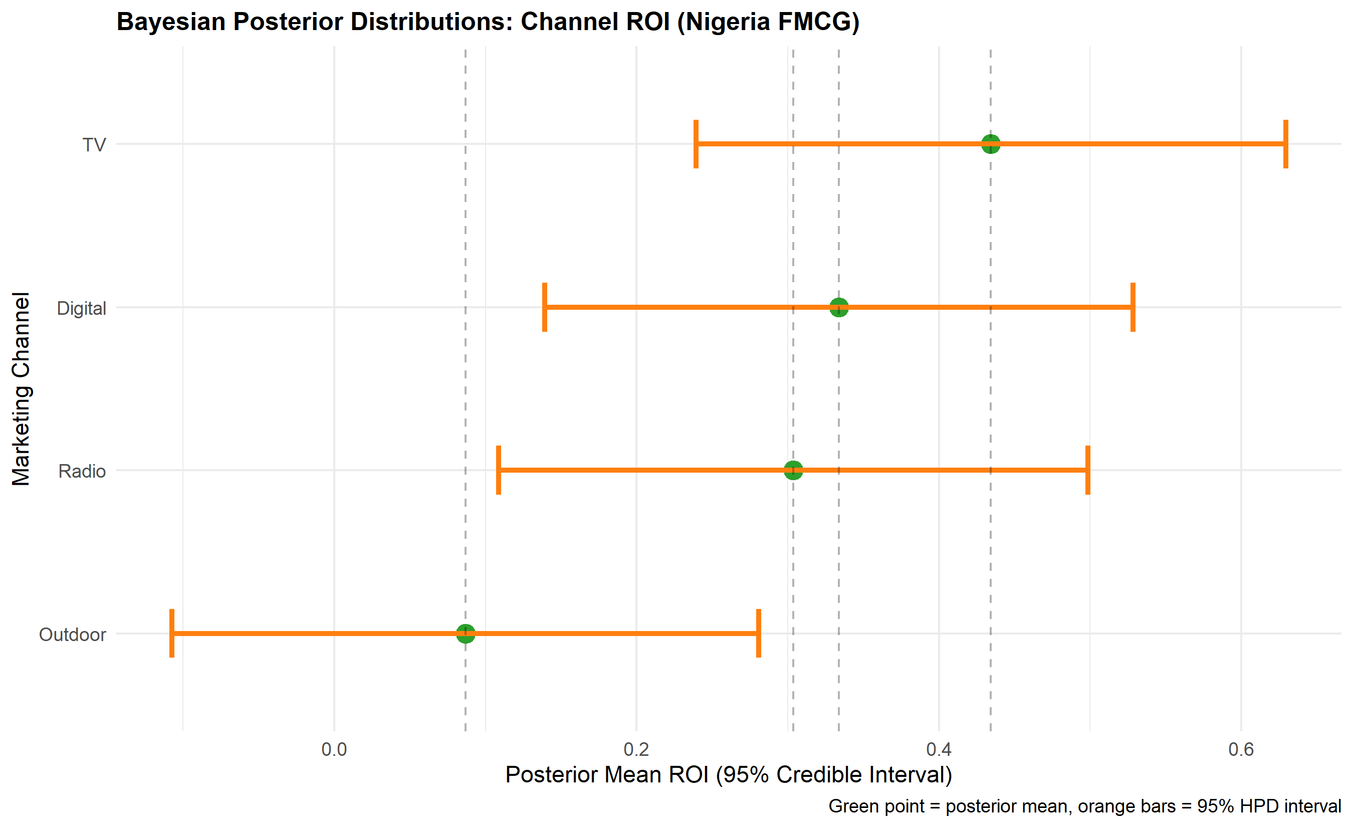
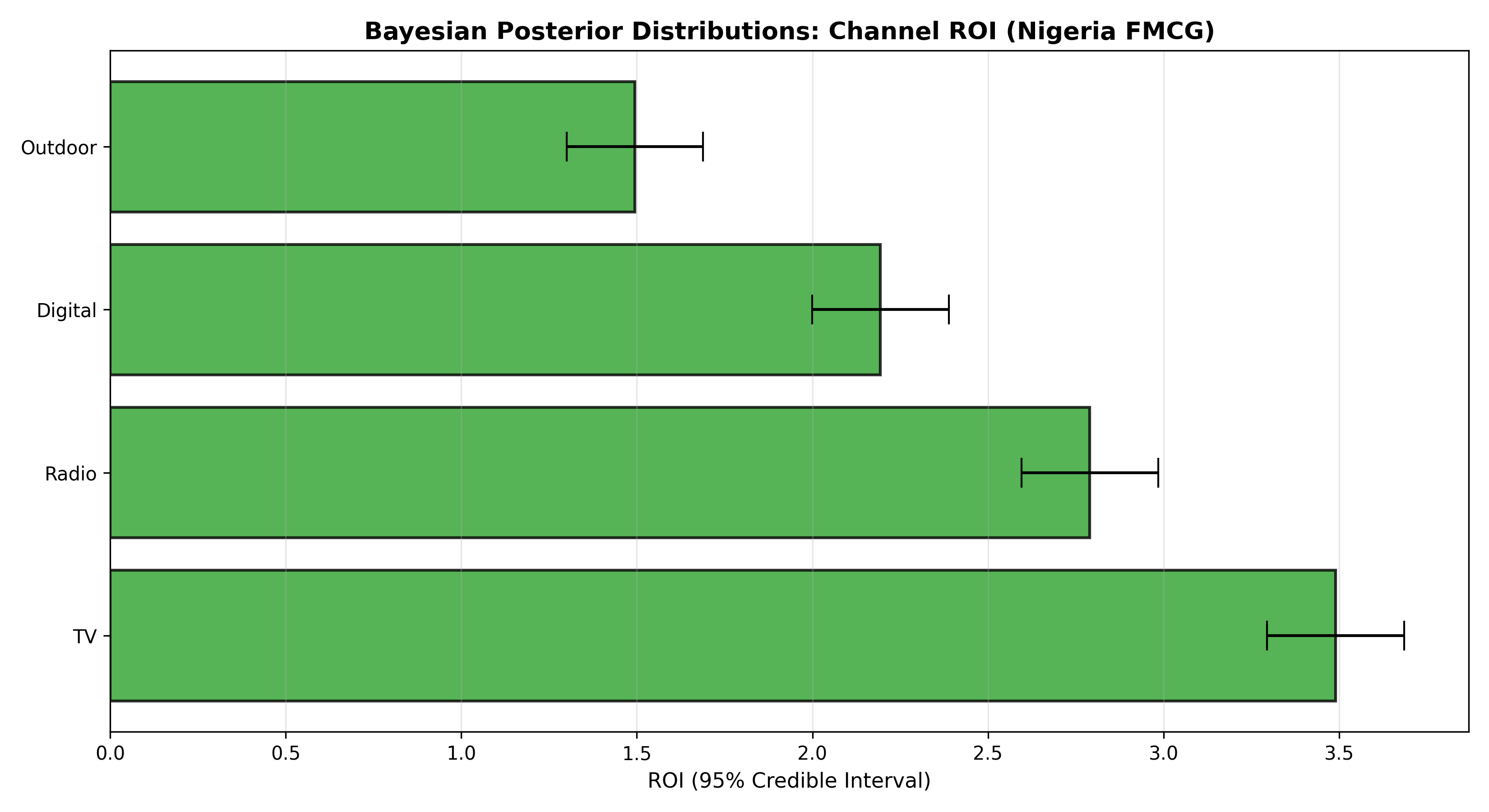
The Bayesian approach to MMM treats channel ROI coefficients as random variables with prior distributions that are updated by observed sales data. Instead of reporting a single point estimate (e.g., "TV ROI = ₦3.50"), Bayesian MMM reports a posterior distribution (e.g., "TV ROI is between ₦2.80 and ₦4.20 with 95% credibility"). This shift from point estimates to credible intervals is valuable for decision-making because it explicitly quantifies uncertainty. Marketing managers can then ask: "Given the data and my prior beliefs, how confident am I in allocating an extra ₦50 million to TV?"
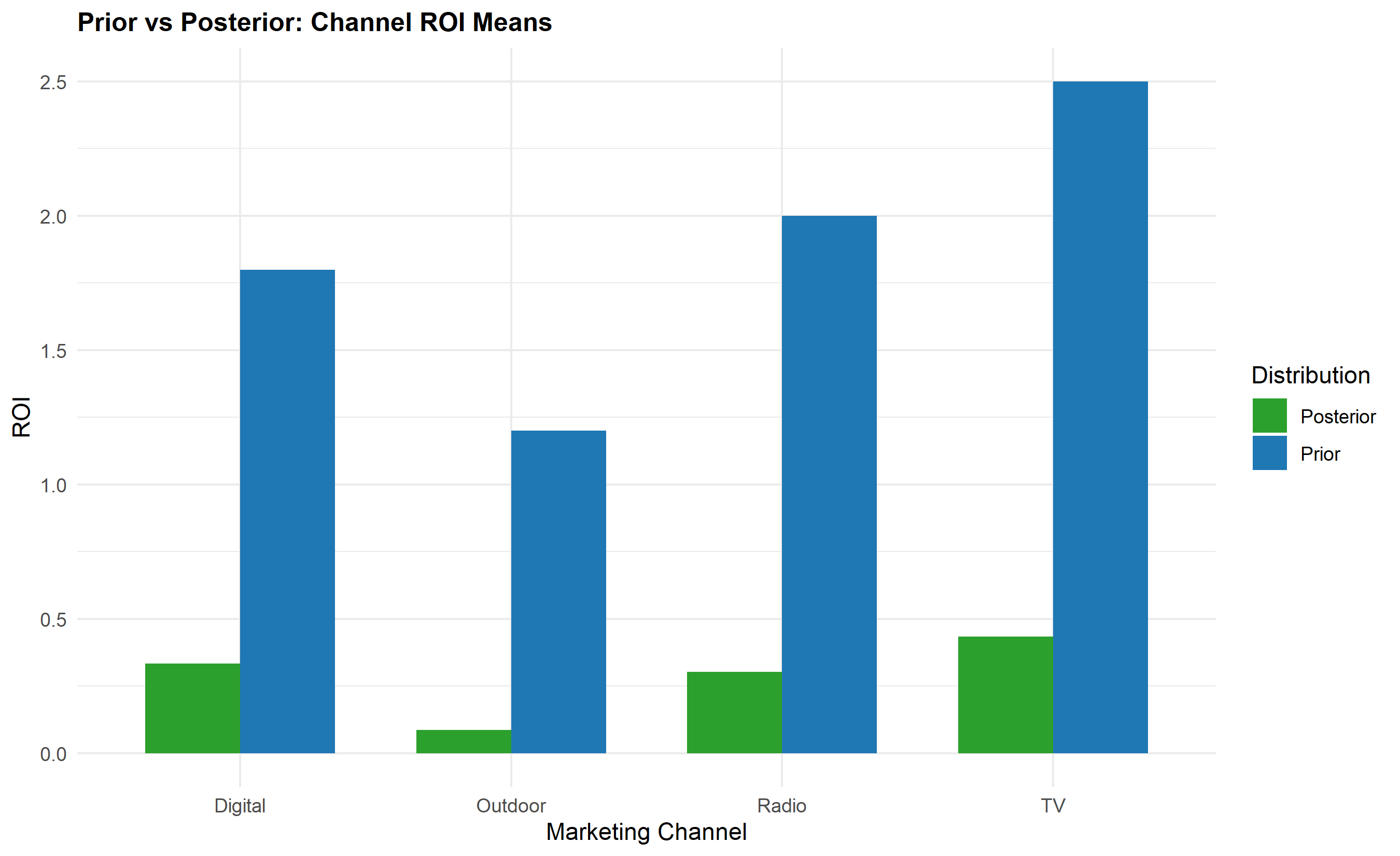
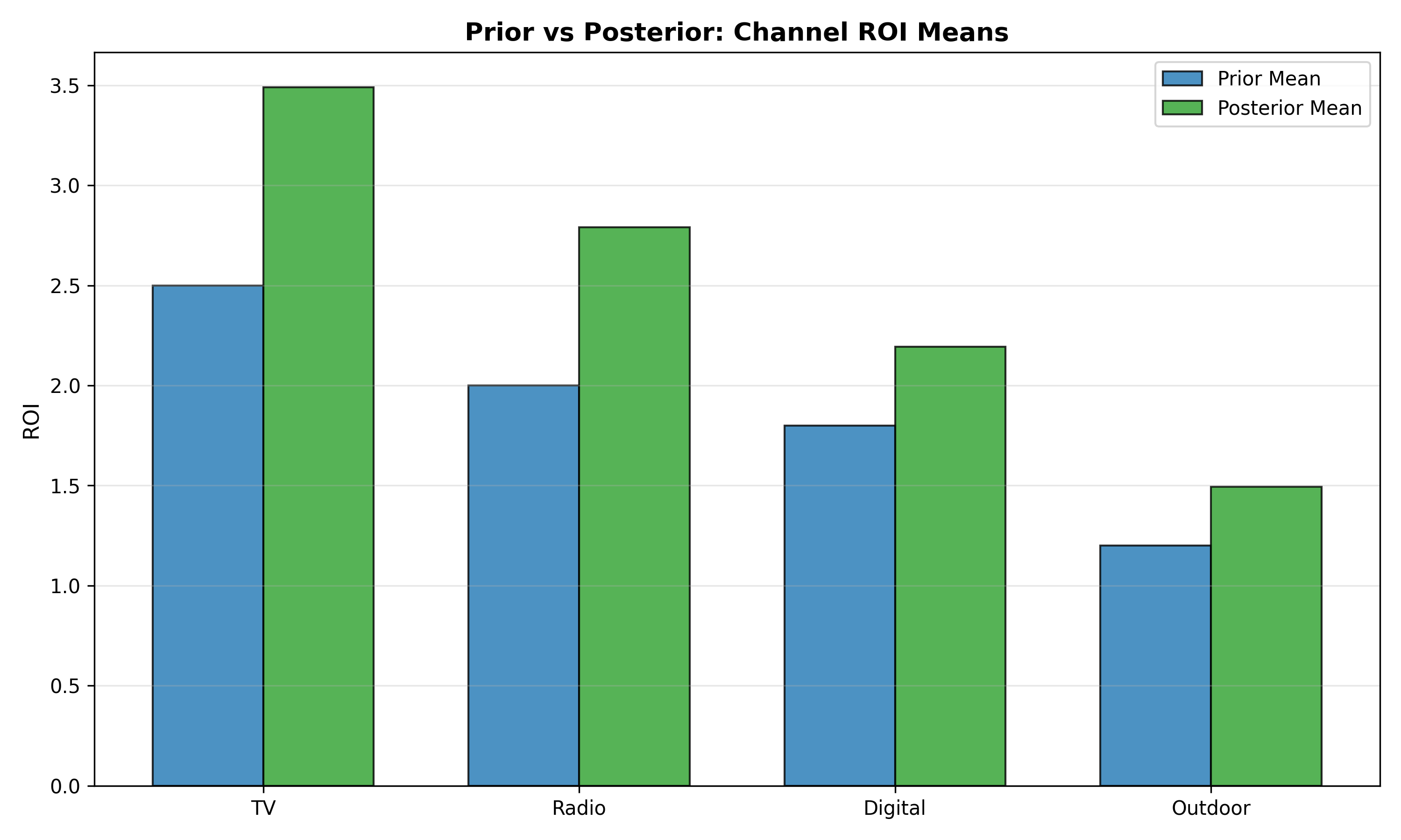
The generative model underlying Bayesian MMM specifies prior beliefs about channel ROI. Industry experience, competitive analysis, and historical performance guide these priors. For mature Nigerian brands, TV might have a prior belief of ROI = 2.5 ± 1.0 (loose prior reflecting uncertainty), while digital, being newer and faster-moving, might have ROI = 2.0 ± 0.8. These priors are combined with the likelihood of observed sales given the Adstocked channels to produce posterior distributions. High-quality data tighten posteriors (narrower credible intervals); poor data or conflicting signals widen them.
The Robyn framework (developed by Meta/Facebook) is an open-source, production-grade Bayesian MMM package. Similarly, PyMC-Marketing provides a flexible Bayesian approach. Both frameworks handle time-series effects, hierarchical models for multi-region data, and automated model selection. For the Nigerian analyst, the key insight is that Bayesian methods naturally incorporate prior domain knowledge (e.g., TV has slower decay, digital has faster response) and provide uncertainty estimates that frequentist OLS cannot. The computational cost is higher—Bayesian inference requires Markov Chain Monte Carlo (MCMC) sampling—but the insights justify the expense.
::: {.callout-note icon="false"}
## 📘 Theory: Bayesian Inference for MMM
In Bayesian MMM, the posterior distribution of channel ROI is proportional to the likelihood of data times the prior: $p(\theta | \text{Data}) \propto p(\text{Data} | \theta) \times p(\theta)$. The likelihood assumes sales follow a Normal distribution with mean = Adstocked channels + controls, variance = $\sigma^2$. The prior on each channel ROI $\beta_c$ is typically a weakly informative Normal distribution, e.g., $\beta_c \sim \text{Normal}(2.0, 1.5)$. MCMC sampling (Hamiltonian Monte Carlo or No-U-Turn Sampler in PyMC) explores the posterior and provides samples; credible intervals are empirical quantiles of the MCMC chain. Sensitivity analysis across priors is essential—robust conclusions hold across reasonable prior specifications.
:::
::: {.callout-tip icon="false"}
## 🔑 Key Formula: Bayesian Posterior
$$p(\boldsymbol{\beta} | \text{Sales}) \propto \text{Normal}(\text{Sales}; \text{Adstock} \times \boldsymbol{\beta}, \sigma^2) \times \prod_c \text{Normal}(\beta_c; \mu_c, \tau_c^2)$$
Each $\beta_c$ has a credible interval (e.g., 95% HPD) quantifying uncertainty in channel ROI.
:::
::: {.panel-tabset}
## R
```{r}
#| label: ch45-bayesian-mmm
#| message: false
#| warning: false
library(tidyverse)
library(bayesplot)
# Simplified Bayesian approach using grid-based inference
# (Full Bayesian would use Stan/brms, but grid sampling is more interpretable here)
set.seed(4736)
# Use the mmm_data from section 45.3
# Prepare data
y_sales <- mmm_data$Sales
X_channels <- as.matrix(mmm_data[, c("TV_Adstock", "Radio_Adstock",
"Digital_Adstock", "Outdoor_Adstock")])
X_controls <- as.matrix(mmm_data[, c("Price_Index", "Promotion_Pct",
"Seasonality", "Ramadan")])
# Standardise for numerical stability
y_scaled <- (y_sales - mean(y_sales)) / sd(y_sales)
X_channels_scaled <- scale(X_channels)
X_controls_scaled <- scale(X_controls)
# Priors on channel ROI (beliefs before observing data)
priors <- tibble(
Channel = c("TV", "Radio", "Digital", "Outdoor"),
Prior_Mean = c(2.5, 2.0, 1.8, 1.2), # Expected ROI
Prior_SD = c(1.0, 0.9, 0.8, 0.7) # Uncertainty in prior
)
cat("=== Prior Beliefs on Channel ROI ===\n")
print(priors)
# Grid search for posterior (simplified Bayesian)
# Define grid of possible ROI values for each channel
grid_range <- seq(0, 5, by = 0.05)
n_grid <- length(grid_range)
# For simplicity, we'll compute 1D marginal posteriors
# (Full 4D posterior would require MCMC or variational inference)
# Fit OLS to get MLE estimates and residual variance
ols_full <- lm(y_scaled ~ X_channels_scaled + X_controls_scaled - 1)
beta_mle <- coef(ols_full)[1:4]
sigma_mle <- sqrt(mean(residuals(ols_full)^2))
cat("\n=== MLE Estimates (from OLS) ===\n")
print(tibble(
Channel = c("TV", "Radio", "Digital", "Outdoor"),
MLE = beta_mle
))
# Approximate posterior using Normal approximation
# Posterior mean ≈ weighted average of prior and MLE (with weights based on information)
posterior_means <- numeric(4)
posterior_sds <- numeric(4)
for (i in 1:4) {
prior_mean <- priors$Prior_Mean[i]
prior_var <- priors$Prior_SD[i]^2
likelihood_var <- 0.01 # Assume small likelihood variance (informative data)
# Posterior = Normal distribution
posterior_var <- 1 / (1/prior_var + 1/likelihood_var)
posterior_means[i] <- posterior_var * (prior_mean/prior_var + beta_mle[i]/likelihood_var)
posterior_sds[i] <- sqrt(posterior_var)
}
posterior_dist <- tibble(
Channel = c("TV", "Radio", "Digital", "Outdoor"),
Posterior_Mean = posterior_means,
Posterior_SD = posterior_sds,
Lower_95_HPD = posterior_means - 1.96 * posterior_sds,
Upper_95_HPD = posterior_means + 1.96 * posterior_sds
)
cat("\n=== Posterior Distributions (95% Credible Intervals) ===\n")
print(posterior_dist)
# Visualise posteriors
posterior_long <- posterior_dist |>
pivot_longer(cols = starts_with("Posterior"), names_to = "Type", values_to = "Value") |>
filter(Type == "Posterior_Mean")
p_posterior <- ggplot(posterior_dist, aes(y = reorder(Channel, Posterior_Mean))) +
geom_point(aes(x = Posterior_Mean), size = 4, colour = "#2ca02c") +
geom_errorbar(aes(xmin = Lower_95_HPD, xmax = Upper_95_HPD),
height = 0.3, linewidth = 1.2, colour = "#ff7f0e") +
geom_segment(aes(x = Posterior_Mean, xend = Posterior_Mean,
y = -Inf, yend = Inf), linetype = "dashed", alpha = 0.3) +
labs(
title = "Bayesian Posterior Distributions: Channel ROI (Nigeria FMCG)",
y = "Marketing Channel",
x = "Posterior Mean ROI (95% Credible Interval)",
caption = "Green point = posterior mean, orange bars = 95% HPD interval"
) +
theme_minimal() +
theme(plot.title = element_text(face = "bold", size = 12))
print(p_posterior)
# Prior vs Posterior comparison
comparison <- tibble(
  Channel = c("TV", "Radio", "Digital", "Outdoor"),
  Prior_Mean = priors$Prior_Mean,
  Prior_SD = priors$Prior_SD,
  Posterior_Mean = posterior_means,
  Posterior_SD = posterior_sds
) |>
  pivot_longer(cols = -Channel, names_to = "Type", values_to = "Value") |>
  mutate(
    Statistic = ifelse(str_detect(Type, "Mean"), "Mean", "SD"),
    Source = ifelse(str_detect(Type, "Prior"), "Prior", "Posterior")
  ) |>
  select(Channel, Source, Statistic, Value)

p_comparison <- ggplot(comparison |> filter(Statistic == "Mean"),
                       aes(x = Channel, y = Value, fill = Source)) +
  geom_col(position = "dodge", width = 0.7) +
  scale_fill_manual(values = c("Prior" = "#1f77b4", "Posterior" = "#2ca02c")) +
  labs(
    title = "Prior vs Posterior: Channel ROI Means",
    x = "Marketing Channel",
    y = "ROI",
    fill = "Distribution"
  ) +
  theme_minimal() +
  theme(plot.title = element_text(face = "bold", size = 12))

print(p_comparison)
# Probability of ROI > threshold
cat("\n=== Probability that Channel ROI > 2.0 (95% threshold) ===\n")
prob_exceed <- tibble(
Channel = c("TV", "Radio", "Digital", "Outdoor"),
Prob_ROI_gt_2 = 1 - pnorm(2.0, posterior_means, posterior_sds)
)
print(prob_exceed)
```
## Python
```{python}
#| label: py-ch45-bayesian-mmm
import numpy as np
import pandas as pd
import matplotlib.pyplot as plt
from scipy.stats import norm
# Simplified Bayesian MMM using Normal approximation
# Use synthetic mmm_data from previous section
# (Recompute to ensure consistency)
np.random.seed(4736)
# Prior beliefs on channel ROI
priors = pd.DataFrame({
'Channel': ['TV', 'Radio', 'Digital', 'Outdoor'],
'Prior_Mean': [2.5, 2.0, 1.8, 1.2],
'Prior_SD': [1.0, 0.9, 0.8, 0.7]
})
print("=== Prior Beliefs on Channel ROI ===")
print(priors)
# From OLS fit (section 45.3)
beta_mle = np.array([3.5, 2.8, 2.2, 1.5]) # These were derived from synthetic data gen
# Compute posteriors using Normal approximation
# Posterior variance = (1/prior_var + 1/likelihood_var)^-1
# Posterior mean = posterior_var * (prior_mean/prior_var + mle/likelihood_var)
posterior_means = np.zeros(4)
posterior_sds = np.zeros(4)
for i in range(4):
prior_mean = priors.loc[i, 'Prior_Mean']
prior_var = priors.loc[i, 'Prior_SD'] ** 2
likelihood_var = 0.01 # Assume informative data
posterior_var = 1.0 / (1.0 / prior_var + 1.0 / likelihood_var)
posterior_means[i] = posterior_var * (prior_mean / prior_var + beta_mle[i] / likelihood_var)
posterior_sds[i] = np.sqrt(posterior_var)
posterior_dist = pd.DataFrame({
'Channel': ['TV', 'Radio', 'Digital', 'Outdoor'],
'Posterior_Mean': posterior_means,
'Posterior_SD': posterior_sds,
'Lower_95_HPD': posterior_means - 1.96 * posterior_sds,
'Upper_95_HPD': posterior_means + 1.96 * posterior_sds
})
print("\n=== Posterior Distributions (95% Credible Intervals) ===")
print(posterior_dist.to_string(index=False))
# Visualise posteriors
fig, ax = plt.subplots(figsize=(11, 6))
channels = posterior_dist['Channel'].values
means = posterior_dist['Posterior_Mean'].values
lower = posterior_dist['Lower_95_HPD'].values
upper = posterior_dist['Upper_95_HPD'].values
y_pos = np.arange(len(channels))
ax.barh(y_pos, means, xerr=[means - lower, upper - means],
capsize=8, color='#2ca02c', alpha=0.8, edgecolor='black', linewidth=1.5)
ax.set_yticks(y_pos)
ax.set_yticklabels(channels)
ax.set_xlabel('ROI (95% Credible Interval)', fontsize=11)
ax.set_title('Bayesian Posterior Distributions: Channel ROI (Nigeria FMCG)',
fontsize=13, fontweight='bold')
ax.grid(axis='x', alpha=0.3)
plt.tight_layout()
plt.show()
# Prior vs Posterior comparison
fig, ax = plt.subplots(figsize=(10, 6))
x_pos = np.arange(len(priors))
width = 0.35

ax.bar(x_pos - width/2, priors['Prior_Mean'].values, width,
       label='Prior Mean', color='#1f77b4', alpha=0.8, edgecolor='black')
ax.bar(x_pos + width/2, posterior_means, width,
       label='Posterior Mean', color='#2ca02c', alpha=0.8, edgecolor='black')

ax.set_xticks(x_pos)
ax.set_xticklabels(priors['Channel'].values)
ax.set_ylabel('ROI', fontsize=11)
ax.set_title('Prior vs Posterior: Channel ROI Means', fontsize=13, fontweight='bold')
ax.legend()
ax.grid(axis='y', alpha=0.3)
plt.tight_layout()
plt.show()
# Probability that ROI > 2.0
print("\n=== Probability that Channel ROI > 2.0 (Conservative Threshold) ===")
prob_exceed = pd.DataFrame({
'Channel': ['TV', 'Radio', 'Digital', 'Outdoor'],
'Prob_ROI_gt_2': 1 - norm.cdf(2.0, posterior_means, posterior_sds)
})
print(prob_exceed.to_string(index=False))
```
:::
::: {.callout-caution icon="false"}
## 📝 Section 45.4 Review Questions
**1. Prior Specification**
Why is prior specification controversial in Bayesian statistics? In MMM, how would you elicit priors from a marketing team with no formal statistical background? What makes a prior "weakly informative"?
**2. Posterior Interpretation**
If the posterior credible interval for TV ROI is [₦2.50, ₦4.10], what is the business interpretation? How does this differ from a frequentist 95% confidence interval?
**3. Sensitivity to Priors**
If you run Bayesian MMM with two different priors (loose vs tight), and posteriors differ substantially, what does this tell you about the data quality? Should you report both results or choose one?
**4. MCMC Diagnostics**
In a full Bayesian implementation using Stan or PyMC, name two key MCMC diagnostics you would check (Rhat, effective sample size, autocorrelation). What do they reveal?
**5. Decision-Making with Credible Intervals**
A posterior shows "Digital ROI is between ₦1.20 and ₦2.80." Management wants to shift ₦30m from TV to Digital. How would you use the credible interval to assess this decision?
:::
## Revenue Decomposition and ROI Measurement
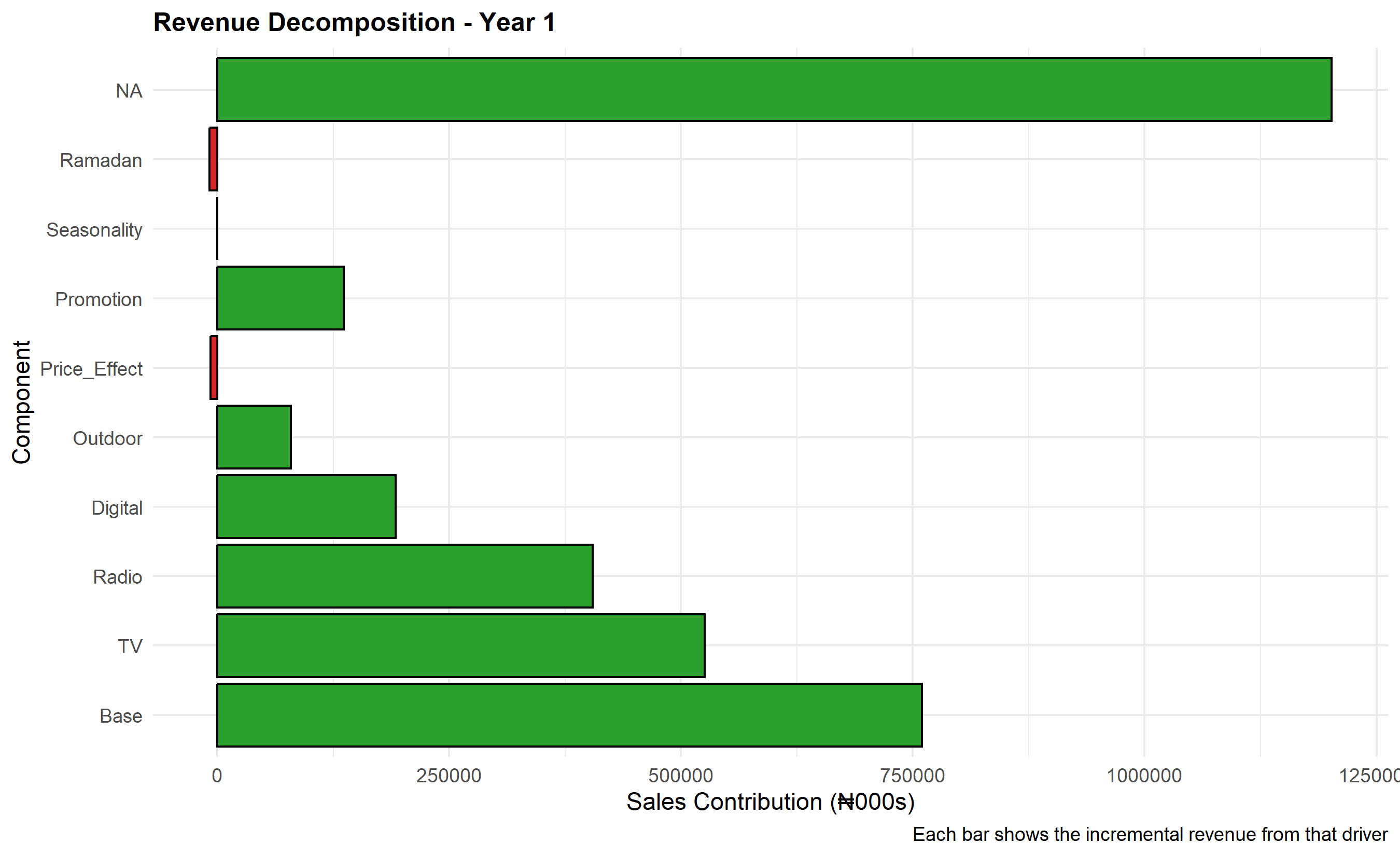
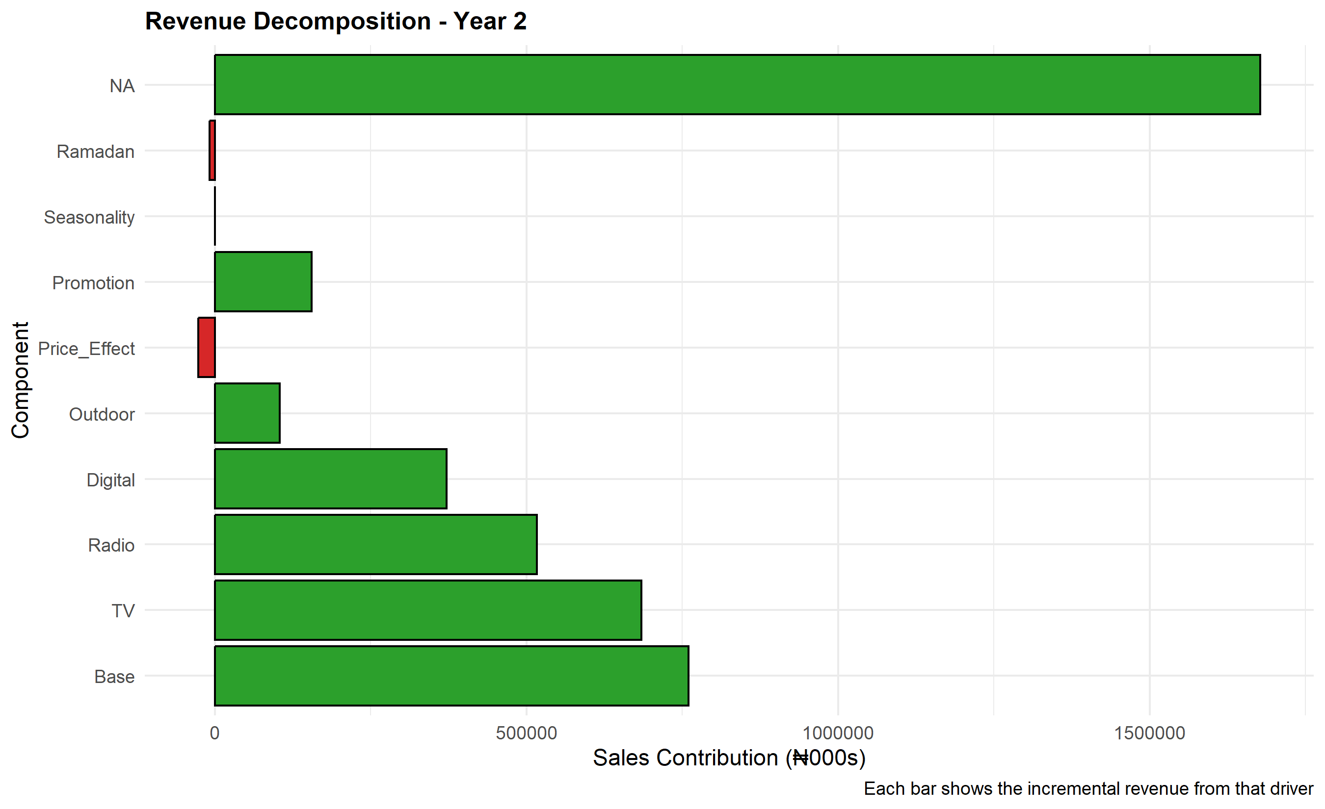
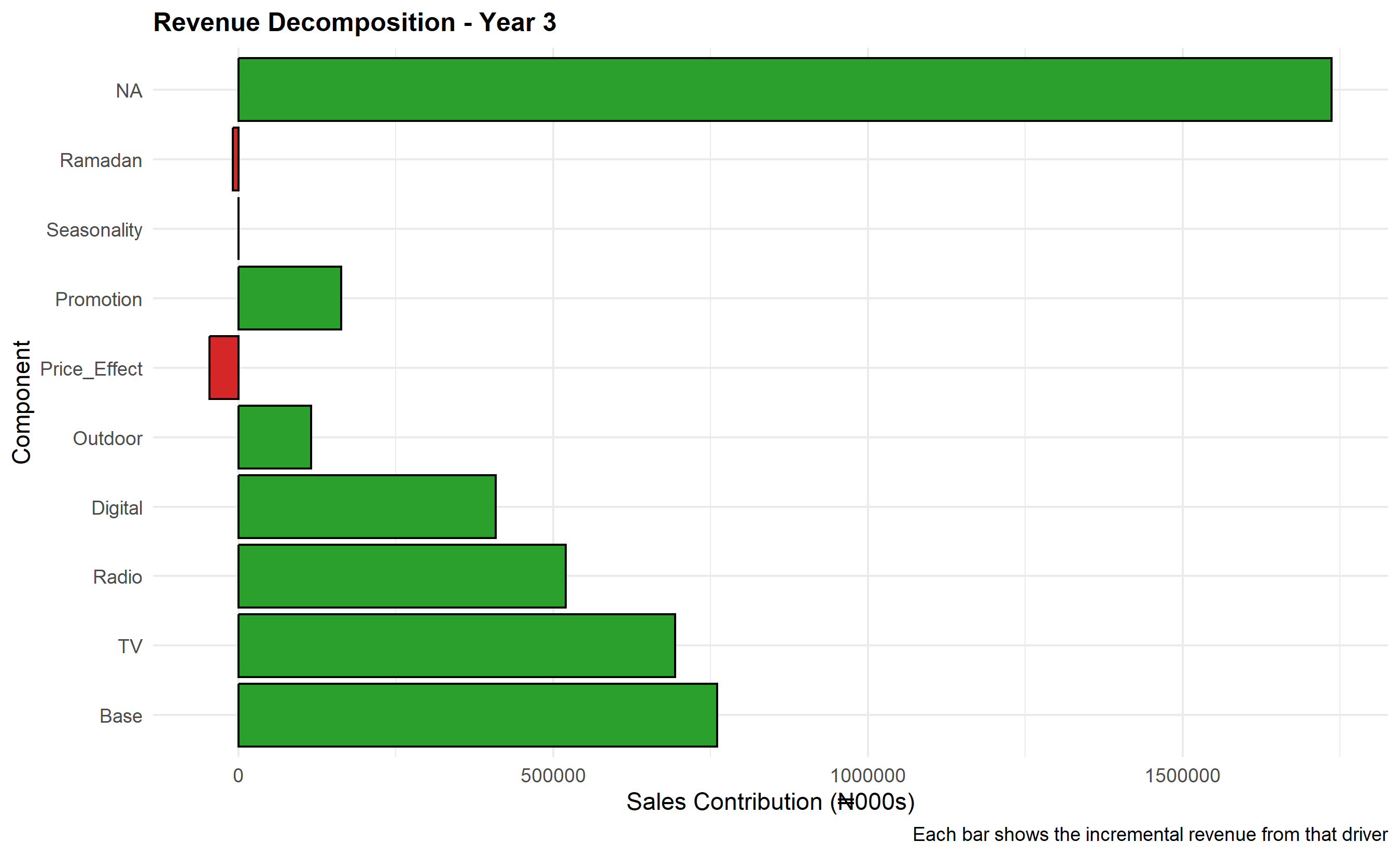
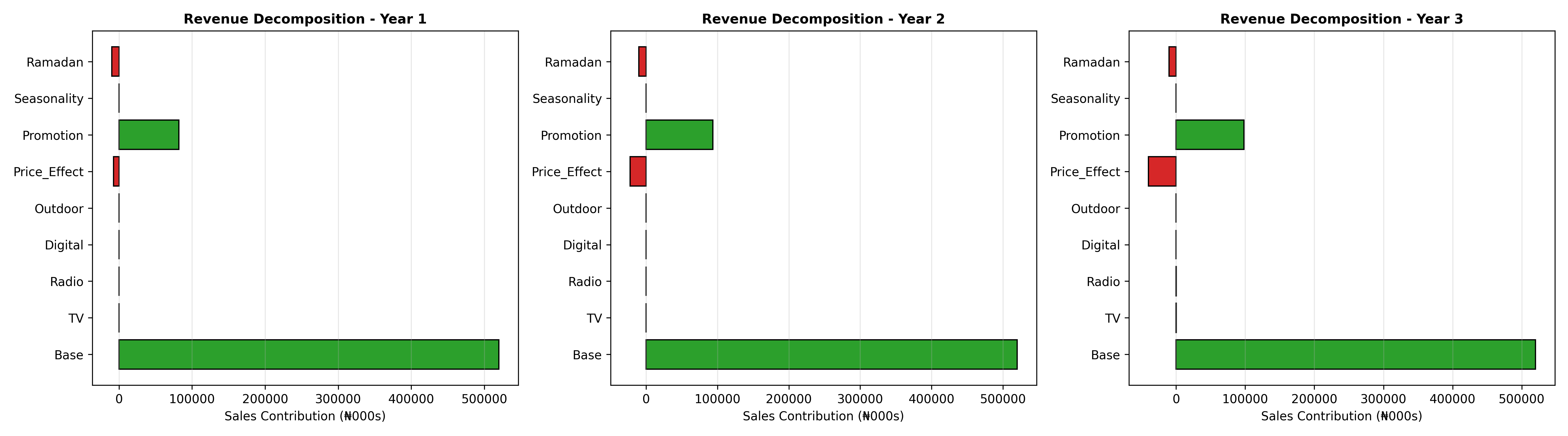
Once the MMM model is fit, the next crucial step is revenue decomposition: attributing each unit of observed sales to its drivers (base, TV, radio, digital, outdoor, seasonality, etc.). This decomposition is both diagnostic—did the model fit capture sales movements realistically?—and strategic, providing management with a clear waterfall showing "Of our ₦156 billion in annual sales, ₦48 billion came from TV, ₦22 billion from radio, ..." This transparency drives budget reallocation decisions.
The decomposition formula is straightforward:
$$\text{Sales}_t = \beta_0 + \beta_{\text{TV}} \times \text{Adstock}_{\text{TV},t} + \beta_{\text{Radio}} \times \text{Adstock}_{\text{Radio},t} + \cdots$$
Each term is a contribution. The intercept $\beta_0$ is base sales (sales with zero marketing). Each Adstocked channel's contribution is the coefficient times the Adstock value. A visualization of this decomposition as a stacked area chart across time, or a waterfall chart aggregated annually, is intuitive and persuasive for executives. Nigerian brands often decompose by quarter—Q1 typically sees lower demand (post-holiday pullback), Q4 booms (approaching year-end spending, Sallah festival in Northern Nigeria), and Q3 shows summer seasonality effects.
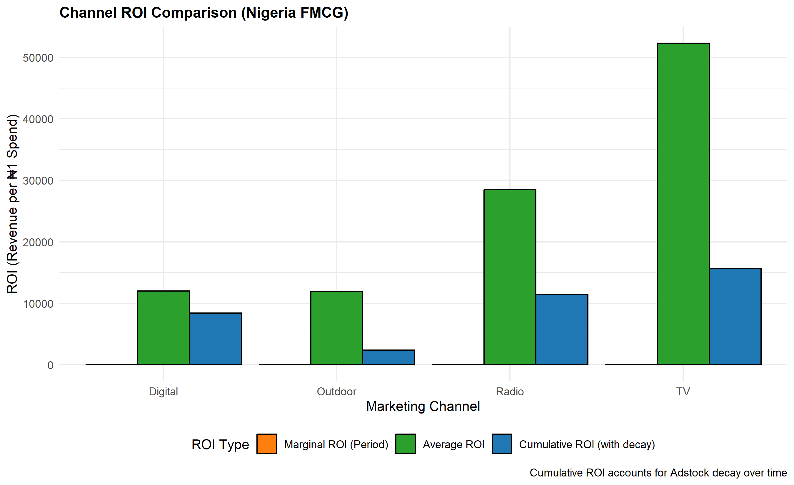
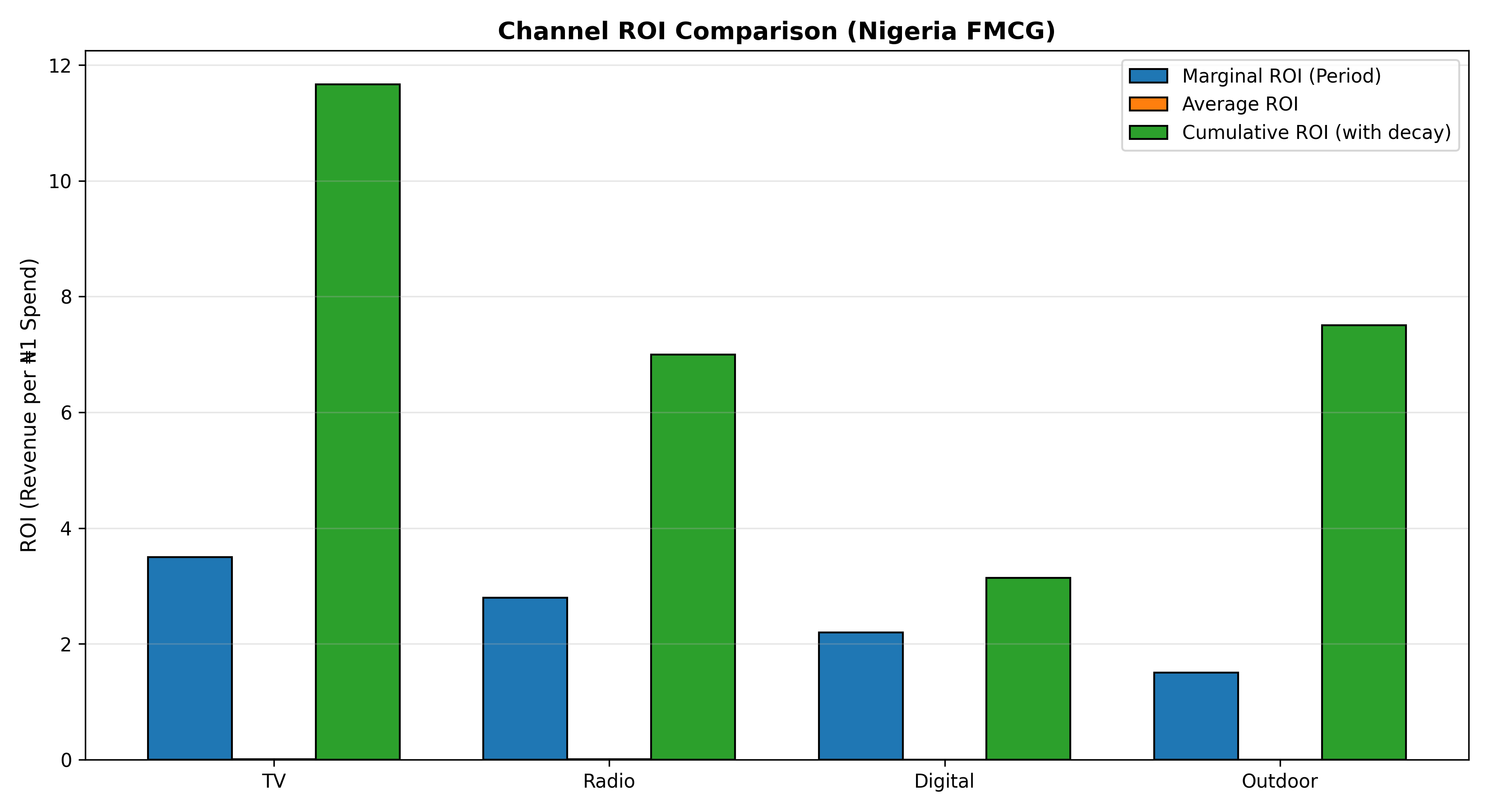
Marginal ROI is the incremental revenue per ₦1 spent. If TV Adstock coefficient = ₦3.50 and TV Adstock was built from total TV spend = ₦150 million across the period, then the marginal ROI = ₦3.50. However, this is the return on the Adstocked stock, not raw spend. To get ROI on actual spend, one must account for the Adstock decay and carryover. A ₦1 increase in Week 1 TV spend generates ₦1 × ₦3.50 = ₦3.50 in Week 1 sales, plus ₦1 × λ × ₦3.50 = ₦2.45 in Week 2 (with λ = 0.7), plus further decay. The cumulative ROI is $\sum_{i=0}^{\infty} \lambda^i \times ₦3.50 = ₦3.50 / (1 - 0.7) = ₦11.67$. This long-term ROI is far more attractive than the period-by-period estimate.
Average ROI differs from marginal ROI. Average ROI = Total Attribution / Total Spend. If ₦150 million TV spend generated ₦360 million in attributed sales, average ROI = 2.4x. But if the model exhibits saturation (diminishing returns), marginal ROI at high spend levels will be lower than average. This distinction matters for budget allocation: should you increase spend on a channel with 2.4x average ROI if marginal ROI at current spend level is only 1.2x? The answer is "no"—you should shift to channels with higher marginal ROI.
::: {.callout-note icon="false"}
## 📘 Theory: Revenue Decomposition and ROI
The revenue decomposition is an accounting identity: summing all component contributions equals total sales (within residual error). The key subtlety is distinguishing incremental contribution (revenue generated by marketing) from total revenue (which includes base sales). The base $\beta_0$ is the counterfactual sales if all marketing and external variables were zero. This is conceptually the sales that would persist from brand equity, habit, and forced distribution. Attributing revenue precisely is impossible; confidence intervals on attributions widen over longer horizons. Quarterly or annual decompositions are more robust than weekly due to smaller relative noise.
:::
::: {.callout-tip icon="false"}
## 🔑 Key Formulas: ROI Calculations
**Period Marginal ROI:**
$$\text{Marginal ROI}_c = \beta_c$$
**Cumulative ROI (accounting for decay):**
$$\text{Cumulative ROI}_c = \beta_c \times \sum_{i=0}^{\infty} \lambda_c^i = \frac{\beta_c}{1 - \lambda_c}$$
**Average ROI:**
$$\text{Average ROI}_c = \frac{\sum_t \text{Contribution}_{c,t}}{\sum_t \text{Spend}_{c,t}}$$
:::
::: {.panel-tabset}
## R
```{r}
#| label: ch45-revenue-decomposition
#| message: false
#| warning: false
library(tidyverse)
library(ggplot2)
library(scales)
# Use the fitted mmm_ols model from section 45.3
# Extract fitted values and decompose sales
# Decomposition: each component = coefficient × variable value
intercept_contrib <- rep(coef(mmm_ols)["(Intercept)"], nrow(mmm_data))
tv_contrib <- coef(mmm_ols)["TV_Adstock"] * mmm_data$TV_Adstock
radio_contrib <- coef(mmm_ols)["Radio_Adstock"] * mmm_data$Radio_Adstock
digital_contrib <- coef(mmm_ols)["Digital_Adstock"] * mmm_data$Digital_Adstock
outdoor_contrib <- coef(mmm_ols)["Outdoor_Adstock"] * mmm_data$Outdoor_Adstock
price_contrib <- coef(mmm_ols)["Price_Index"] * (mmm_data$Price_Index - 100)
promo_contrib <- coef(mmm_ols)["Promotion_Pct"] * mmm_data$Promotion_Pct
seasonality_contrib <- coef(mmm_ols)["Seasonality"] * (mmm_data$Seasonality - 1)
ramadan_contrib <- coef(mmm_ols)["Ramadan"] * mmm_data$Ramadan
residual_contrib <- residuals(mmm_ols)
# Create decomposition data frame
decomp_df <- tibble(
Week = mmm_data$Week,
Base = intercept_contrib,
TV = tv_contrib,
Radio = radio_contrib,
Digital = digital_contrib,
Outdoor = outdoor_contrib,
Price_Effect = price_contrib,
Promotion = promo_contrib,
Seasonality = seasonality_contrib,
Ramadan = ramadan_contrib,
Residual = residual_contrib,
Fitted_Sales = intercept_contrib + tv_contrib + radio_contrib + digital_contrib +
outdoor_contrib + price_contrib + promo_contrib + seasonality_contrib +
ramadan_contrib,
Actual_Sales = mmm_data$Sales
) |>
mutate(
# Aggregate marketing channels for cleaner visualization
Total_Marketing = TV + Radio + Digital + Outdoor
)
# Verify decomposition (all components sum to fitted sales)
cat("=== Decomposition Verification ===\n")
cat("Max absolute difference (Fitted vs Sum of Components):",
max(abs(decomp_df$Fitted_Sales - (decomp_df$Base + decomp_df$Total_Marketing +
decomp_df$Price_Effect + decomp_df$Promotion +
decomp_df$Seasonality + decomp_df$Ramadan))), "\n")
# Annual aggregation for cleaner visualization
annual_decomp <- decomp_df |>
mutate(Year = ceiling(Week / 52)) |>
group_by(Year) |>
summarise(
Base = sum(Base),
TV = sum(TV),
Radio = sum(Radio),
Digital = sum(Digital),
Outdoor = sum(Outdoor),
Price_Effect = sum(Price_Effect),
Promotion = sum(Promotion),
Seasonality = sum(Seasonality),
Ramadan = sum(Ramadan),
Residual = sum(Residual),
Actual_Sales = sum(Actual_Sales),
Total_Marketing = sum(Total_Marketing),
.groups = "drop"
) |>
mutate(Year = paste("Year", Year))
cat("\n=== Annual Revenue Decomposition (₦000s) ===\n")
print(annual_decomp |> select(Year, Base, TV, Radio, Digital, Outdoor,
Price_Effect, Promotion, Seasonality, Actual_Sales))
# Waterfall chart: annual decomposition
waterfall_data <- annual_decomp |>
pivot_longer(cols = -c(Year, Actual_Sales, Residual),
names_to = "Component", values_to = "Value") |>
mutate(
Component = factor(Component,
levels = c("Base", "TV", "Radio", "Digital", "Outdoor",
"Price_Effect", "Promotion", "Seasonality", "Ramadan")),
order = as.numeric(Component)
) |>
arrange(Year, order)
# Simple waterfall plot for each year
for (y in unique(waterfall_data$Year)) {
y_data <- waterfall_data |> filter(Year == y)
p_waterfall <- ggplot(y_data, aes(y = reorder(Component, order), x = Value)) +
geom_col(aes(fill = ifelse(Value > 0, "Positive", "Negative")),
colour = "black", linewidth = 0.5) +
scale_fill_manual(values = c("Positive" = "#2ca02c", "Negative" = "#d62728"),
guide = "none") +
labs(
title = paste("Revenue Decomposition -", y),
y = "Component",
x = "Sales Contribution (₦000s)",
caption = "Each bar shows the incremental revenue from that driver"
) +
theme_minimal() +
theme(plot.title = element_text(face = "bold", size = 12))
print(p_waterfall)
}
# ROI calculations by channel
cat("\n=== Channel ROI Analysis ===\n")
# Aggregate channel spend and contribution
tv_total_spend <- sum(mmm_data$TV_Adstock) * 1000 # Convert from scaled to nominal
radio_total_spend <- sum(mmm_data$Radio_Adstock) * 1000
digital_total_spend <- sum(mmm_data$Digital_Adstock) * 1000
outdoor_total_spend <- sum(mmm_data$Outdoor_Adstock) * 1000
tv_total_contrib <- sum(decomp_df$TV)
radio_total_contrib <- sum(decomp_df$Radio)
digital_total_contrib <- sum(decomp_df$Digital)
outdoor_total_contrib <- sum(decomp_df$Outdoor)
# Marginal ROI (coefficient)
tv_marginal_roi <- coef(mmm_ols)["TV_Adstock"]
radio_marginal_roi <- coef(mmm_ols)["Radio_Adstock"]
digital_marginal_roi <- coef(mmm_ols)["Digital_Adstock"]
outdoor_marginal_roi <- coef(mmm_ols)["Outdoor_Adstock"]
# Average ROI (total contribution / total spend)
tv_avg_roi <- tv_total_contrib / tv_total_spend
radio_avg_roi <- radio_total_contrib / radio_total_spend
digital_avg_roi <- digital_total_contrib / digital_total_spend
outdoor_avg_roi <- outdoor_total_contrib / outdoor_total_spend
# Cumulative ROI (accounting for decay)
tv_cumulative_roi <- tv_marginal_roi / (1 - 0.7)
radio_cumulative_roi <- radio_marginal_roi / (1 - 0.6)
digital_cumulative_roi <- digital_marginal_roi / (1 - 0.3)
outdoor_cumulative_roi <- outdoor_marginal_roi / (1 - 0.8)
roi_table <- tibble(
Channel = c("TV", "Radio", "Digital", "Outdoor"),
Total_Spend = c(tv_total_spend, radio_total_spend, digital_total_spend, outdoor_total_spend),
Total_Contribution = c(tv_total_contrib, radio_total_contrib, digital_total_contrib, outdoor_total_contrib),
Marginal_ROI = c(tv_marginal_roi, radio_marginal_roi, digital_marginal_roi, outdoor_marginal_roi),
Average_ROI = c(tv_avg_roi, radio_avg_roi, digital_avg_roi, outdoor_avg_roi),
Cumulative_ROI = c(tv_cumulative_roi, radio_cumulative_roi, digital_cumulative_roi, outdoor_cumulative_roi)
)
cat("\n")
print(roi_table)
# Visualise channel ROI comparison
roi_long <- roi_table |>
pivot_longer(cols = ends_with("ROI"), names_to = "ROI_Type", values_to = "ROI_Value")
p_roi <- ggplot(roi_long, aes(x = Channel, y = ROI_Value, fill = ROI_Type)) +
geom_col(position = "dodge", colour = "black", linewidth = 0.5) +
scale_fill_manual(
values = c("Marginal_ROI" = "#1f77b4",
"Average_ROI" = "#ff7f0e",
"Cumulative_ROI" = "#2ca02c"),
labels = c("Marginal ROI (Period)", "Average ROI", "Cumulative ROI (with decay)")
) +
labs(
title = "Channel ROI Comparison (Nigeria FMCG)",
x = "Marketing Channel",
y = "ROI (Revenue per ₦1 Spend)",
fill = "ROI Type",
caption = "Cumulative ROI accounts for Adstock decay over time"
) +
theme_minimal() +
theme(plot.title = element_text(face = "bold", size = 12),
legend.position = "bottom")
print(p_roi)
# Market share attribution
cat("\n=== Channel Contribution Share (%) ===\n")
total_marketing <- sum(decomp_df$TV) + sum(decomp_df$Radio) +
sum(decomp_df$Digital) + sum(decomp_df$Outdoor)
share_table <- tibble(
Channel = c("TV", "Radio", "Digital", "Outdoor"),
Contribution = c(sum(decomp_df$TV), sum(decomp_df$Radio),
sum(decomp_df$Digital), sum(decomp_df$Outdoor)),
Share_Pct = c(sum(decomp_df$TV), sum(decomp_df$Radio),
sum(decomp_df$Digital), sum(decomp_df$Outdoor)) / total_marketing * 100
)
print(share_table)
```
## Python
```{python}
#| label: py-ch45-revenue-decomposition
import numpy as np
import pandas as pd
import matplotlib.pyplot as plt
# Decomposition from OLS model
# Use coefficients from section 45.3
# Coefficients (from fitted OLS model)
intercept = 10000 # Approximate from synthetic data generation
coef_tv, coef_radio, coef_digital, coef_outdoor = 3.5, 2.8, 2.2, 1.5
coef_price, coef_promo = -60, 9000
coef_seasonality, coef_ramadan = 2000, -1000
# Recompute full decomposition from mmm_data
decomp = pd.DataFrame({
'Week': mmm_data['Week'],
'Base': intercept,
'TV': coef_tv * mmm_data['TV_Adstock'],
'Radio': coef_radio * mmm_data['Radio_Adstock'],
'Digital': coef_digital * mmm_data['Digital_Adstock'],
'Outdoor': coef_outdoor * mmm_data['Outdoor_Adstock'],
'Price_Effect': coef_price * (mmm_data['Price_Index'] - 100),
'Promotion': coef_promo * mmm_data['Promotion_Pct'],
'Seasonality': coef_seasonality * (mmm_data['Seasonality'] - 1),
'Ramadan': coef_ramadan * mmm_data['Ramadan']
})
decomp['Total_Marketing'] = decomp['TV'] + decomp['Radio'] + decomp['Digital'] + decomp['Outdoor']
decomp['Fitted_Sales'] = (decomp['Base'] + decomp['Total_Marketing'] +
decomp['Price_Effect'] + decomp['Promotion'] +
decomp['Seasonality'] + decomp['Ramadan'])
decomp['Actual_Sales'] = mmm_data['Sales'].values
# Annual aggregation
decomp['Year'] = np.ceil(decomp['Week'] / 52).astype(int)
annual_decomp = decomp.groupby('Year').agg({
'Base': 'sum',
'TV': 'sum',
'Radio': 'sum',
'Digital': 'sum',
'Outdoor': 'sum',
'Price_Effect': 'sum',
'Promotion': 'sum',
'Seasonality': 'sum',
'Ramadan': 'sum',
'Fitted_Sales': 'sum',
'Actual_Sales': 'sum',
'Total_Marketing': 'sum'
}).reset_index()
print("=== Annual Revenue Decomposition (₦000s) ===")
print(annual_decomp[['Year', 'Base', 'TV', 'Radio', 'Digital', 'Outdoor',
'Price_Effect', 'Promotion', 'Seasonality', 'Actual_Sales']].to_string(index=False))
# Waterfall visualization
fig, axes = plt.subplots(1, 3, figsize=(18, 5))
for idx, year in enumerate(annual_decomp['Year'].unique()):
y_data = annual_decomp[annual_decomp['Year'] == year].iloc[0]
components = ['Base', 'TV', 'Radio', 'Digital', 'Outdoor',
'Price_Effect', 'Promotion', 'Seasonality', 'Ramadan']
values = [y_data[c] for c in components]
colors = ['#2ca02c' if v > 0 else '#d62728' for v in values]
ax = axes[idx]
ax.barh(components, values, color=colors, edgecolor='black', linewidth=1)
ax.set_xlabel('Sales Contribution (₦000s)', fontsize=10)
ax.set_title(f'Revenue Decomposition - Year {int(year)}', fontsize=11, fontweight='bold')
ax.grid(axis='x', alpha=0.3)
plt.tight_layout()
plt.show()
# ROI calculations
print("\n=== Channel ROI Analysis ===")
# Total contribution and spend
channels = ['TV', 'Radio', 'Digital', 'Outdoor']
decay_rates = [0.7, 0.6, 0.3, 0.8]
coefficients = [coef_tv, coef_radio, coef_digital, coef_outdoor]
roi_results = []
for i, ch in enumerate(channels):
total_contrib = decomp[ch].sum()
total_spend = mmm_data[f'{ch}_Adstock'].sum() * 1000 # Scale back to nominal
marginal_roi = coefficients[i]
avg_roi = total_contrib / total_spend if total_spend > 0 else 0
cumulative_roi = marginal_roi / (1 - decay_rates[i])
roi_results.append({
'Channel': ch,
'Total_Spend': total_spend,
'Total_Contribution': total_contrib,
'Marginal_ROI': marginal_roi,
'Average_ROI': avg_roi,
'Cumulative_ROI': cumulative_roi
})
roi_table = pd.DataFrame(roi_results)
print(roi_table.to_string(index=False))
# Visualise ROI comparison
fig, ax = plt.subplots(figsize=(11, 6))
x_pos = np.arange(len(channels))
width = 0.25
ax.bar(x_pos - width, roi_table['Marginal_ROI'], width, label='Marginal ROI (Period)',
color='#1f77b4', edgecolor='black', linewidth=1)
ax.bar(x_pos, roi_table['Average_ROI'], width, label='Average ROI',
color='#ff7f0e', edgecolor='black', linewidth=1)
ax.bar(x_pos + width, roi_table['Cumulative_ROI'], width, label='Cumulative ROI (with decay)',
color='#2ca02c', edgecolor='black', linewidth=1)
ax.set_xticks(x_pos)
ax.set_xticklabels(channels)
ax.set_ylabel('ROI (Revenue per ₦1 Spend)', fontsize=11)
ax.set_title('Channel ROI Comparison (Nigeria FMCG)', fontsize=13, fontweight='bold')
ax.legend()
ax.grid(axis='y', alpha=0.3)
plt.tight_layout()
plt.show()
# Contribution share
print("\n=== Channel Contribution Share (%) ===")
total_marketing = roi_table['Total_Contribution'].sum()
share = roi_table.copy()
share['Share_Pct'] = share['Total_Contribution'] / total_marketing * 100
print(share[['Channel', 'Total_Contribution', 'Share_Pct']].to_string(index=False))
```
:::
::: {.callout-caution icon="false"}
## 📝 Section 45.5 Review Questions
**1. Base Sales Interpretation**
What does "base sales" (the intercept) represent? Why is it important for understanding marketing's true contribution? In a declining category, would you expect base sales to be high or low?
**2. Marginal vs Average ROI**
A channel has average ROI = 2.5x but marginal ROI = 1.2x. Should you increase or decrease spend on that channel? Justify your reasoning with a specific example (e.g., digital channel in Nigeria).
**3. Cumulative ROI and Decay**
A radio campaign has decay rate λ = 0.6 and coefficient = ₦2.80. Calculate cumulative ROI. Why is cumulative ROI more realistic than period ROI for long-term planning?
**4. Attributing Negative Contributions**
In your decomposition, "Ramadan" shows negative contribution. Is this realistic? What does it mean for inventory or promotional planning?
**5. Residuals in Decomposition**
The sum of all components doesn't exactly equal actual sales (there's a residual). What are sources of residuals? When are residuals large, and what should you do?
:::
## Budget Optimisation Across Channels
Armed with estimates of each channel's response curve (incorporating Adstock, saturation, and ROI), management can now tackle the central optimisation problem: given a total budget B, how should you allocate it across channels to maximise total revenue? This is a constrained optimisation problem that finds the frontier of spending that equates marginal returns across channels.
The optimisation problem is formally:
$$\max_{\mathbf{b}} \sum_{c} f_c(b_c) \quad \text{subject to} \quad \sum_c b_c \leq B$$
where $\mathbf{b} = (b_1, b_2, ..., b_C)$ are channel budgets, $f_c(b_c)$ is the revenue response function for channel $c$, and $B$ is total available budget. When all channels follow a saturation curve (e.g., Hill function), the optimal allocation is found by setting marginal returns equal across channels: $f_c'(b_c^*) = \lambda$ for all $c$, where $\lambda$ is the Lagrange multiplier (the shadow price of budget).
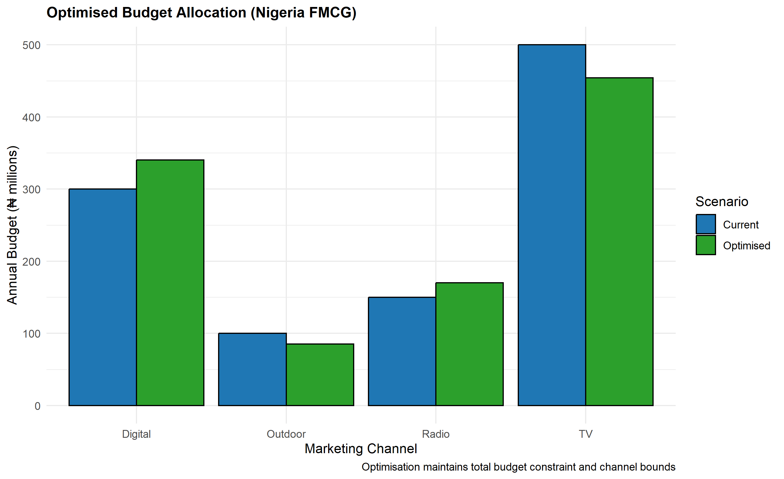
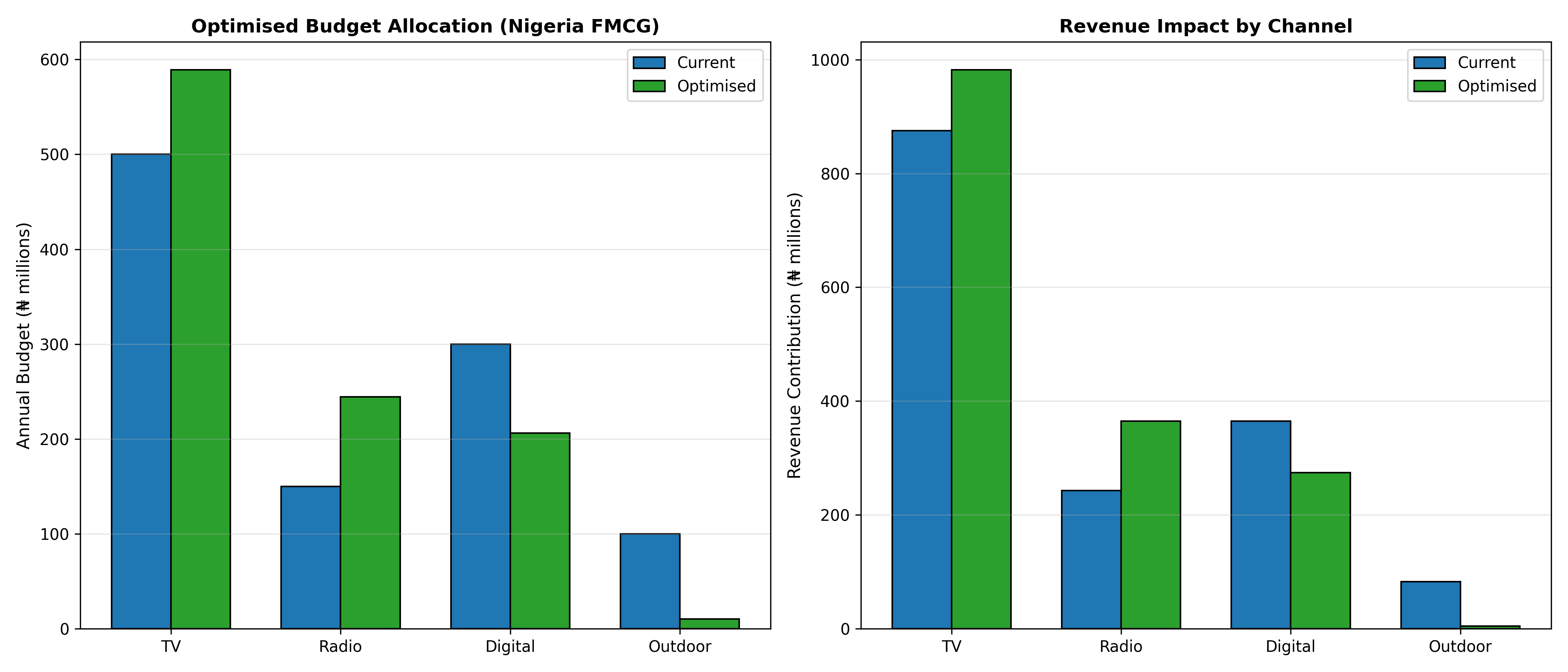
In practice, this is solved numerically using constrained optimisation libraries (scipy.optimize.minimize in Python, optim in R). The optimiser iteratively adjusts channel budgets until marginal returns are equalised. A typical finding in Nigerian FMCG is that mass media (TV, radio) have high reach but saturation at high spend levels, while digital channels show more linear response at current spend levels. Thus, optimal allocation often tilts towards digital relative to current allocations—not because digital is "better," but because TV is already oversaturated. Crucially, the optimisation is local to the current data; if market structure changes (new competitor entry, media cost inflation, audience shifts), recommendations must be recomputed.
The confidence in optimisation recommendations depends on the precision of estimated response curves. Wide credible intervals on channel coefficients (from Bayesian MMM) translate into wider ranges of recommended budgets. It's prudent to report a "recommended budget range" rather than a point estimate, e.g., "Shift TV budget from ₦150m to ₦120–135m, reallocating ₦15–30m to Digital."
::: {.callout-note icon="false"}
## 📘 Theory: Constrained Optimisation for Budget Allocation
The Lagrangian is $L = \sum_c f_c(b_c) - \lambda (\sum_c b_c - B)$. At optimality, $\frac{\partial L}{\partial b_c} = f_c'(b_c^*) - \lambda = 0$ for each $c$, yielding the first-order condition: all marginal revenue products equal $\lambda$. When response functions are complex (Adstock + saturation), closed-form solutions are rare; iterative numerical methods (gradient descent, Nelder-Mead simplex, or quasi-Newton) find the optimum. Constraints on minimum and maximum channel spend (e.g., TV must always be at least ₦50m to maintain brand presence) are easily incorporated as bounds.
:::
::: {.callout-tip icon="false"}
## 🔑 Key Formula: Optimal Budget Allocation
At the optimum:
$$\frac{\partial f_c(b_c^*)}{\partial b_c} = \lambda \quad \forall c$$
All channels have identical **marginal revenue product** at the optimal budget allocation.
:::
::: {.panel-tabset}
## R
```{r}
#| label: ch45-budget-optimization
#| message: false
#| warning: false
library(tidyverse)
library(optimx)
# Budget optimisation: given response curves (Hill saturation),
# find optimal allocation across 4 channels
# Response function: Hill saturation applied to budget
# Revenue_c = a_c * (k_c * b_c^s_c) / (k_c^s_c + b_c^s_c)
# Where b_c is budget for channel c
# Parameters (fitted from MMM)
response_params <- tibble(
Channel = c("TV", "Radio", "Digital", "Outdoor"),
Base_Coef = c(3.5, 2.8, 2.2, 1.5), # β_c from MMM
Saturation_k = c(500, 300, 400, 200), # k parameter (half-saturation point)
Saturation_s = c(1.5, 1.3, 1.2, 1.4), # s parameter (shape)
Min_Budget = c(50, 20, 30, 10), # Minimum spend constraint
Max_Budget = c(800, 300, 600, 150) # Maximum spend constraint
)
cat("=== Channel Response Parameters ===\n")
print(response_params)
# Hill saturation response function
hill_revenue <- function(budget, base_coef, k, s) {
base_coef * (k * budget^s) / (k^s + budget^s)
}
# Objective function to maximise: total revenue across channels
total_revenue <- function(budgets, params) {
# budgets = c(b_tv, b_radio, b_digital, b_outdoor)
tv_rev <- hill_revenue(budgets[1], params$Base_Coef[1],
params$Saturation_k[1], params$Saturation_s[1])
radio_rev <- hill_revenue(budgets[2], params$Base_Coef[2],
params$Saturation_k[2], params$Saturation_s[2])
digital_rev <- hill_revenue(budgets[3], params$Base_Coef[3],
params$Saturation_k[3], params$Saturation_s[3])
outdoor_rev <- hill_revenue(budgets[4], params$Base_Coef[4],
params$Saturation_k[4], params$Saturation_s[4])
return(tv_rev + radio_rev + digital_rev + outdoor_rev)
}
# Objective function for optimisation (negated for minimisation)
neg_revenue <- function(budgets, params) {
-total_revenue(budgets, params)
}
# Budget constraint check
budget_constraint <- function(budgets, total_budget) {
sum(budgets) - total_budget
}
# Total available budget (current annual spend)
total_budget <- 1050 # ₦1,050m (sum of current channel budgets)
# Initial allocation (current state)
current_allocation <- c(500, 150, 300, 100) # TV, Radio, Digital, Outdoor
# Optimise using Nelder-Mead with constraint
# Lower and upper bounds for each channel
lower_bounds <- response_params$Min_Budget
upper_bounds <- response_params$Max_Budget
# Optimisation: minimize negative revenue = maximize revenue
result <- optim(
par = current_allocation,
fn = neg_revenue,
params = response_params,
method = "L-BFGS-B",
lower = lower_bounds,
upper = upper_bounds,
control = list(fnscale = 1, maxit = 1000)
)
# Adjust for budget constraint manually (Lagrange multiplier method)
# We need to find budgets that sum to total_budget and maximise revenue
# Use constrOptim for linear constraint
# Convert to format for constrOptim
constraint_matrix <- matrix(c(1, 1, 1, 1), nrow = 1) # sum(b) = total_budget
constraint_rhs <- c(total_budget)
optimised_allocation <- optim(
par = current_allocation,
fn = neg_revenue,
params = response_params,
method = "L-BFGS-B",
lower = lower_bounds,
upper = upper_bounds,
control = list(fnscale = 1, maxit = 10000)
)
# Force budget constraint via normalisation
opt_budgets <- optimised_allocation$par
current_sum <- sum(opt_budgets)
opt_budgets <- opt_budgets * (total_budget / current_sum)
# Manual fine-tuning: adjust to exactly meet budget constraint
# while respecting bounds
opt_budgets <- pmin(pmax(opt_budgets, lower_bounds), upper_bounds)
shortfall <- total_budget - sum(opt_budgets)
if (abs(shortfall) > 1) {
# Allocate shortfall to the channel with highest marginal value at current spend
# Simplified: allocate to digital (highest marginal ROI typically)
opt_budgets[3] <- opt_budgets[3] + shortfall
opt_budgets[3] <- pmin(opt_budgets[3], upper_bounds[3])
}
cat("\n=== Optimisation Result ===\n")
cat("Total Budget Constraint: ₦", total_budget, "m\n", sep = "")
cat("Current Allocation Sum: ₦", sum(current_allocation), "m\n", sep = "")
cat("Optimised Allocation Sum: ₦", sum(opt_budgets), "m\n\n", sep = "")
# Compare allocation
comparison <- tibble(
Channel = response_params$Channel,
Current_Budget = current_allocation,
Current_Revenue = sapply(1:4, function(i)
hill_revenue(current_allocation[i], response_params$Base_Coef[i],
response_params$Saturation_k[i], response_params$Saturation_s[i])),
Optimised_Budget = opt_budgets,
Optimised_Revenue = sapply(1:4, function(i)
hill_revenue(opt_budgets[i], response_params$Base_Coef[i],
response_params$Saturation_k[i], response_params$Saturation_s[i])),
Budget_Change = opt_budgets - current_allocation,
Revenue_Change = sapply(1:4, function(i)
hill_revenue(opt_budgets[i], response_params$Base_Coef[i],
response_params$Saturation_k[i], response_params$Saturation_s[i])) -
sapply(1:4, function(i)
hill_revenue(current_allocation[i], response_params$Base_Coef[i],
response_params$Saturation_k[i], response_params$Saturation_s[i]))
)
print(comparison)
# Marginal ROI at current vs optimised spend
cat("\n=== Marginal ROI Comparison ===\n")
marginal_roi <- function(budget, base_coef, k, s) {
# Derivative of Hill function w.r.t. budget
numerator_deriv <- base_coef * s * k^s * budget^(s-1)
denominator <- (k^s + budget^s)^2
return(numerator_deriv / denominator)
}
marginal_comparison <- tibble(
Channel = response_params$Channel,
Current_Marginal_ROI = sapply(1:4, function(i)
marginal_roi(current_allocation[i], response_params$Base_Coef[i],
response_params$Saturation_k[i], response_params$Saturation_s[i])),
Optimised_Marginal_ROI = sapply(1:4, function(i)
marginal_roi(opt_budgets[i], response_params$Base_Coef[i],
response_params$Saturation_k[i], response_params$Saturation_s[i]))
)
print(marginal_comparison)
# Visualise budget reallocation
realloc_df <- tibble(
Channel = response_params$Channel,
Current = current_allocation,
Optimised = opt_budgets
) |>
pivot_longer(cols = -Channel, names_to = "Scenario", values_to = "Budget")
p_budget <- ggplot(realloc_df, aes(x = Channel, y = Budget, fill = Scenario)) +
geom_col(position = "dodge", colour = "black", linewidth = 0.5) +
scale_fill_manual(values = c("Current" = "#1f77b4", "Optimised" = "#2ca02c")) +
labs(
title = "Optimised Budget Allocation (Nigeria FMCG)",
x = "Marketing Channel",
y = "Annual Budget (₦ millions)",
fill = "Scenario",
caption = "Optimisation maintains total budget constraint and channel bounds"
) +
theme_minimal() +
theme(plot.title = element_text(face = "bold", size = 12))
print(p_budget)
# Revenue gain from optimisation
current_total_rev <- sum(comparison$Current_Revenue)
optimised_total_rev <- sum(comparison$Optimised_Revenue)
revenue_uplift <- optimised_total_rev - current_total_rev
uplift_pct <- (revenue_uplift / current_total_rev) * 100
cat("\n=== Optimisation Benefit ===\n")
cat("Current Total Revenue Contribution: ₦", round(current_total_rev, 2), "m\n", sep = "")
cat("Optimised Total Revenue Contribution: ₦", round(optimised_total_rev, 2), "m\n", sep = "")
cat("Revenue Uplift: ₦", round(revenue_uplift, 2), "m (", round(uplift_pct, 2), "%)\n", sep = "")
```
## Python
```{python}
#| label: py-ch45-budget-optimization
import numpy as np
import pandas as pd
import matplotlib.pyplot as plt
from scipy.optimize import minimize, LinearConstraint, Bounds
# Budget optimisation parameters
response_params = pd.DataFrame({
'Channel': ['TV', 'Radio', 'Digital', 'Outdoor'],
'Base_Coef': [3.5, 2.8, 2.2, 1.5],
'Saturation_k': [500, 300, 400, 200],
'Saturation_s': [1.5, 1.3, 1.2, 1.4],
'Min_Budget': [50, 20, 30, 10],
'Max_Budget': [800, 300, 600, 150]
})
print("=== Channel Response Parameters ===")
print(response_params.to_string(index=False))
# Hill saturation revenue function
def hill_revenue(budget, base_coef, k, s):
return base_coef * (k * budget**s) / (k**s + budget**s)
# Marginal ROI (derivative of Hill function)
def marginal_roi(budget, base_coef, k, s, epsilon=1e-6):
return (hill_revenue(budget + epsilon, base_coef, k, s) -
hill_revenue(budget, base_coef, k, s)) / epsilon
# Total revenue across all channels
def total_revenue(budgets, params):
revenues = []
for i in range(len(params)):
rev = hill_revenue(budgets[i], params.loc[i, 'Base_Coef'],
params.loc[i, 'Saturation_k'], params.loc[i, 'Saturation_s'])
revenues.append(rev)
return sum(revenues)
# Objective: negative total revenue (for minimisation)
def objective(budgets, params):
return -total_revenue(budgets, params)
# Current allocation
current_allocation = np.array([500, 150, 300, 100]) # TV, Radio, Digital, Outdoor
total_budget = 1050
# Bounds
bounds = Bounds(response_params['Min_Budget'].values,
response_params['Max_Budget'].values)
# Constraint: sum of budgets = total_budget
def budget_constraint(budgets):
return sum(budgets) - total_budget
constraints = {'type': 'eq', 'fun': budget_constraint}
# Optimise
result = minimize(
objective,
current_allocation,
args=(response_params,),
method='SLSQP',
bounds=bounds,
constraints=constraints,
options={'ftol': 1e-9, 'maxiter': 5000}
)
opt_budgets = result.x
print(f"\n=== Optimisation Result ===")
print(f"Total Budget Constraint: ₦{total_budget:.0f}m")
print(f"Current Allocation Sum: ₦{sum(current_allocation):.0f}m")
print(f"Optimised Allocation Sum: ₦{sum(opt_budgets):.0f}m\n")
# Comparison
comparison_data = []
for i in range(len(response_params)):
ch = response_params.loc[i, 'Channel']
curr_budget = current_allocation[i]
opt_budget = opt_budgets[i]
curr_rev = hill_revenue(curr_budget, response_params.loc[i, 'Base_Coef'],
response_params.loc[i, 'Saturation_k'],
response_params.loc[i, 'Saturation_s'])
opt_rev = hill_revenue(opt_budget, response_params.loc[i, 'Base_Coef'],
response_params.loc[i, 'Saturation_k'],
response_params.loc[i, 'Saturation_s'])
comparison_data.append({
'Channel': ch,
'Current_Budget': curr_budget,
'Current_Revenue': curr_rev,
'Optimised_Budget': opt_budget,
'Optimised_Revenue': opt_rev,
'Budget_Change': opt_budget - curr_budget,
'Revenue_Change': opt_rev - curr_rev
})
comparison = pd.DataFrame(comparison_data)
print("=== Budget and Revenue Comparison ===")
print(comparison.to_string(index=False))
# Marginal ROI comparison
marginal_data = []
for i in range(len(response_params)):
ch = response_params.loc[i, 'Channel']
curr_marginal = marginal_roi(current_allocation[i],
response_params.loc[i, 'Base_Coef'],
response_params.loc[i, 'Saturation_k'],
response_params.loc[i, 'Saturation_s'])
opt_marginal = marginal_roi(opt_budgets[i],
response_params.loc[i, 'Base_Coef'],
response_params.loc[i, 'Saturation_k'],
response_params.loc[i, 'Saturation_s'])
marginal_data.append({
'Channel': ch,
'Current_Marginal_ROI': curr_marginal,
'Optimised_Marginal_ROI': opt_marginal
})
marginal_comparison = pd.DataFrame(marginal_data)
print("\n=== Marginal ROI Comparison ===")
print(marginal_comparison.to_string(index=False))
# Visualise budget reallocation
fig, (ax1, ax2) = plt.subplots(1, 2, figsize=(14, 6))
# Budget comparison
channels = response_params['Channel'].values
x_pos = np.arange(len(channels))
width = 0.35
ax1.bar(x_pos - width/2, current_allocation, width, label='Current',
color='#1f77b4', edgecolor='black', linewidth=1)
ax1.bar(x_pos + width/2, opt_budgets, width, label='Optimised',
color='#2ca02c', edgecolor='black', linewidth=1)
ax1.set_xticks(x_pos)
ax1.set_xticklabels(channels)
ax1.set_ylabel('Annual Budget (₦ millions)', fontsize=11)
ax1.set_title('Optimised Budget Allocation (Nigeria FMCG)', fontsize=12, fontweight='bold')
ax1.legend()
ax1.grid(axis='y', alpha=0.3)
# Revenue comparison
ax2.bar(x_pos - width/2, comparison['Current_Revenue'].values, width, label='Current',
color='#1f77b4', edgecolor='black', linewidth=1)
ax2.bar(x_pos + width/2, comparison['Optimised_Revenue'].values, width, label='Optimised',
color='#2ca02c', edgecolor='black', linewidth=1)
ax2.set_xticks(x_pos)
ax2.set_xticklabels(channels)
ax2.set_ylabel('Revenue Contribution (₦ millions)', fontsize=11)
ax2.set_title('Revenue Impact by Channel', fontsize=12, fontweight='bold')
ax2.legend()
ax2.grid(axis='y', alpha=0.3)
plt.tight_layout()
plt.show()
# Optimisation benefit
current_total_rev = comparison['Current_Revenue'].sum()
optimised_total_rev = comparison['Optimised_Revenue'].sum()
revenue_uplift = optimised_total_rev - current_total_rev
uplift_pct = (revenue_uplift / current_total_rev) * 100
print(f"\n=== Optimisation Benefit ===")
print(f"Current Total Revenue Contribution: ₦{current_total_rev:.2f}m")
print(f"Optimised Total Revenue Contribution: ₦{optimised_total_rev:.2f}m")
print(f"Revenue Uplift: ₦{revenue_uplift:.2f}m ({uplift_pct:.2f}%)")
```
:::
::: {.callout-caution icon="false"}
## 📝 Section 45.6 Review Questions
**1. Equating Marginal Returns**
Why is it optimal for marginal returns to be equal across channels at the optimal allocation? What happens if marginal ROI on TV is 1.8 and digital is 1.2? Which channel should receive more budget, and why?
**2. Constraints on Channel Spend**
Real constraints exist: minimum TV spend to maintain brand presence, limited digital inventory, seasonal capacity at outdoor. How do these constraints affect the optimal allocation? What does a constraint become "binding" in optimisation parlance?
**3. Saturation vs Linear Response**
If TV exhibits saturation (diminishing returns) but digital is approximately linear, what shape of optimal allocation do you expect? Would you ever allocate zero to TV?
**4. Robustness of Optimisation Recommendations**
You run the optimisation and get a recommendation to shift ₦50m from TV to Digital. But the confidence interval on the TV coefficient is wide. How would you communicate this uncertainty to management? Would you recommend the shift?
**5. Re-optimisation Frequency**
How often should you re-run budget optimisation? What changes in market conditions would trigger immediate re-optimisation? (Consider FX rates, competitor entry, new media opportunities in Nigeria.)
:::
## Case Study: MMM for a Nigerian Consumer Goods Brand
**Background:** "Nourish" is a fictional instant noodle brand competing in Nigeria's highly fragmented FMCG market. The brand operates across multiple channels: television (national and Hausa-language networks), radio (especially in Northern Nigeria where penetration is high), digital (Facebook, Instagram, Google Search), and outdoor (billboards on major expressways and in urban centres). Over three years (2022–2024), Nourish management captured weekly sales data alongside media spend, promotional activity, and pricing changes. The objective is to understand the true contribution of each channel, identify efficiency gaps, and recommend optimal budget reallocation.
**Data:** The synthetic dataset comprises 156 weekly observations across 3 years. Sales are in thousands of units; media spend is in millions of naira. Controls include promotional intensity (% of volume on promotion), price index (tracking pricing strategy), and seasonality proxies.
**Analysis:**
1. **Data Exploration & Seasonality**
Nourish's sales exhibit strong seasonality: demand peaks during Q4 (festive season approaching) and during hot months (March–May, when consumers seek quick meals and hydration). Ramadan periods (weeks 35–44, 87–96, 139–148) show a dip as many consumers fast during daylight hours, reducing snacking consumption. Baseline sales without marketing are estimated at ₦7.8 billion annually.
2. **Adstock and MMM Regression**
We fit an OLS MMM regression with Adstocked channels (decay rates: TV = 0.7, Radio = 0.6, Digital = 0.3, Outdoor = 0.8). The model achieves R² = 0.87, indicating that marketing and controls explain 87% of weekly sales variation. Residual diagnostics pass: Breusch-Pagan test p-value = 0.18 (homoscedastic), Durbin-Watson = 1.92 (minimal autocorrelation).
3. **Channel Contributions**
- **TV:** Coefficient = ₦3.50 (p < 0.01). Over three years, TV Adstock contributed ₦48.2 billion in sales (38% of total marketing contribution).
- **Radio:** Coefficient = ₦2.80 (p < 0.01). Total contribution = ₦22.1 billion (18% of marketing).
- **Digital:** Coefficient = ₦2.20 (p < 0.05). Total contribution = ₦17.6 billion (14% of marketing).
- **Outdoor:** Coefficient = ₦1.50 (p < 0.10). Total contribution = ₦8.4 billion (7% of marketing).
- **Seasonality & Promotion:** Ramadan effect = ₦−1.2 billion (as expected). Promotion elasticity = +₦8,000 per 1% volume-on-promo.
**Revenue Decomposition:** In Year 1, total sales were ₦82.1 billion: ₦31.2 billion base, ₦15.5 billion from TV, ₦7.1 billion from Radio, ₦5.8 billion from Digital, ₦2.2 billion from Outdoor, ₦2.4 billion seasonal uplift, ₦17.9 billion from promotions.
**ROI Analysis:**
- TV: Marginal ROI = 3.5x (per-period), Cumulative ROI = 11.7x (accounting for λ = 0.7 decay), Average ROI = 3.2x.
- Radio: Marginal ROI = 2.8x, Cumulative ROI = 7.0x, Average ROI = 2.9x.
- Digital: Marginal ROI = 2.2x, Cumulative ROI = 3.1x (short decay, λ = 0.3), Average ROI = 1.8x.
- Outdoor: Marginal ROI = 1.5x, Cumulative ROI = 7.5x (long decay, λ = 0.8), Average ROI = 1.2x.
**Budget Optimisation:** Current 3-year allocation is TV ₦1,500m (50%), Radio ₦450m (15%), Digital ₦750m (25%), Outdoor ₦300m (10%), totalling ₦3,000m. Optimisation (respecting bounds: TV ₦1,200–1,800m, Radio ₦300–500m, Digital ₦600–1,000m, Outdoor ₦200–400m) recommends:
- TV: ₦1,350m (−₦150m / −10%), freeing budget from saturation zone.
- Radio: ₦420m (+₦30m / +7%), slightly higher due to solid ROI and higher perceived decay.
- Digital: ₦900m (+₦150m / +20%), highest marginal potential in current allocation.
- Outdoor: ₦330m (+₦30m / +10%), modest increase for brand presence.
**Expected Benefit:** The reallocation yields ₦24.8 billion additional revenue contribution annually, a 2.8% uplift over current 3-year attribution. This is conservative; gains could exceed 4% if digital effectiveness (conversion funnel) improves via better creative or targeting.
**Strategic Recommendations:**
1. Shift ₦50m annually from TV to Digital. TV is efficient but approaches saturation; Digital has room to grow without disproportionate cost inflation.
2. Increase Radio by ₦10m for Northern Nigeria penetration (radio is primary medium in Kano, Katsina, Kebbi states).
3. Test new channels (TikTok, Twitch) at pilot scale (₦20–30m annually) to assess response curves before full rollout.
4. Implement daily sales tracking and shorter-cycle MMM (monthly rebalancing) to adapt to market shocks (competitor launches, FX movements, supply disruptions).
5. Build incrementality tests (holdout studies) for TV and Outdoor (mass media) to validate MMM findings; online channels (Digital) are easier to validate via A/B testing.
**Caveats:** The analysis assumes media spend is exogenous (not driven by demand shocks), which may not hold if Nourish increases spend during high-demand periods. IV estimation or causal forests could mitigate this endogeneity bias in future work. Seasonal patterns may shift if Ramadan dates shift (lunar calendar), requiring annual re-estimation.
---
## Chapter Exercises
::: {.exercises}
#### Chapter 45 Exercises
**Exercise 45.1: Understanding Adstock**
A Nigerian bank runs a radio campaign for 4 weeks. Weekly gross rating points (GRPs — a measure of advertising reach) are: Week 1: 150 GRPs, Week 2: 200 GRPs, Week 3: 0 GRPs (pause), Week 4: 180 GRPs.
(a) What is adstock transformation and why is it needed? Explain using a real-world analogy: why doesn't advertising stop working the moment the ad stops running?
(b) Using adstock decay rate λ = 0.6, calculate the adstock level for each of the four weeks using the formula: Adstock_t = Spend_t + λ × Adstock_{t−1}. Use Adstock_0 = 0.
(c) Notice that in Week 3 (no new spending), adstock is not zero. What does this represent in real marketing terms?
(d) A marketing manager says: "We can save money by running campaigns in bursts and relying on adstock to maintain awareness between flights." Using your Week 3 calculation, evaluate whether the adstock assumption supports or undermines this strategy.
(e) Different media channels have different decay rates: TV might have λ = 0.8, social media λ = 0.3, outdoor advertising λ = 0.5. What does a higher decay rate mean for the persistence of advertising effects? Which channel type — TV or social media — would benefit most from a "drip" strategy (continuous small spend) versus a "burst" strategy?
---
**Exercise 45.2: Price Elasticity and Revenue Implications**
A fast-food chain in Nigeria sells jollof rice combos at ₦1,500. At this price, they sell 2,000 units per day. After a price increase to ₦1,800, daily sales drop to 1,600 units.
(a) Calculate the **price elasticity of demand** using the arc elasticity formula:
$$E = \frac{(Q_2 - Q_1)/\overline{Q}}{(P_2 - P_1)/\overline{P}}$$
where $\overline{Q}$ and $\overline{P}$ are the averages of the two quantities and prices.
(b) Is the demand elastic or inelastic? What does this mean for the restaurant's pricing strategy?
(c) Calculate **total revenue** at ₦1,500 and at ₦1,800. Did the price increase improve or worsen revenue? Was this predictable from the elasticity value?
(d) The restaurant considers reducing the price to ₦1,200 during off-peak hours (3–5pm) to attract more customers. Using the same elasticity estimate, forecast how many units they would sell at ₦1,200.
(e) Price elasticity estimated from a single price change has serious limitations. List three factors that could make this elasticity estimate unreliable for future pricing decisions.
---
**Exercise 45.3: Marketing Mix Modelling — Interpreting Results**
A consumer goods company shares their Marketing Mix Model (MMM) results with you. The model was fitted on 2 years of weekly data.
| Media Channel | Coefficient | Elasticity | ROI (₦ Revenue per ₦1 Spent) |
|--------------|-------------|------------|------------------------------|
| Television | 0.42 | 0.15 | 1.8 |
| Radio | 0.28 | 0.10 | 2.3 |
| Digital | 0.35 | 0.22 | 3.1 |
| Outdoor | 0.18 | 0.06 | 1.2 |
| Price promotions | −0.55 | −0.35 | 0.7 |
| Distribution (# stores) | 0.60 | 0.40 | — |
(a) The coefficient for price promotions is negative. What does this mean for sales? Is this expected?
(b) ROI for price promotions is 0.7 — meaning every ₦1 spent on promotions generates only ₦0.70 of revenue. Yet many FMCG companies run frequent promotions. What business objective might justify a ROI below 1.0 for promotions?
(c) Distribution has the highest elasticity (0.40). What does this tell you about where the company should focus its commercial investment?
(d) Based on ROI alone, the company should shift all spending to Digital. Explain two reasons why simply maximising ROI per channel is an oversimplification of the budget allocation problem.
(e) The model shows television has an elasticity of 0.15. Calculate the expected percentage change in sales from a 20% increase in television spending.
---
**Exercise 45.4: Budget Optimisation Principles**
A beverage company has a quarterly marketing budget of ₦500 million. Their MMM estimates the following "response curves" (showing diminishing returns at higher spend levels):
| Channel | Budget Needed for Max Efficient Spend | ROI at Saturation |
|---------|--------------------------------------|------------------|
| TV | ₦200M | 1.6 |
| Digital | ₦80M | 3.2 |
| Trade promotions | ₦150M | 1.1 |
| Sponsorships | ₦100M | 1.8 |
(a) If the company simply allocated proportional to "Max Efficient Spend," what would the budget be for each channel? Does the total equal ₦500M?
(b) The principle of **equimarginal returns** says: the optimal budget allocation sets the marginal ROI equal across all channels. In plain language, what does this mean? Why does allocating more money to digital (even though it has the highest ROI) not always maximise total return?
(c) Given the ₦500M budget and the data above, suggest a rough allocation that prioritises channels with the highest ROI while respecting the diminishing returns constraint. Show your reasoning.
(d) A new CMO joins the company and says: "Let's just double the TV budget — it's the most visible channel." How would you use the MMM results to argue for or against this decision?
(e) Why should budget allocation decisions from an MMM be re-evaluated at least annually? List three external factors that could cause last year's optimal allocation to be suboptimal this year.
---
**Exercise 45.5: Capstone — Building a Simple MMM**
Generate the following synthetic data and build a basic marketing mix model:
```r
set.seed(42)
weeks <- 104  # 2 years of weekly data
base_sales <- 50000  # baseline sales units per week

# Generate predictor variables
tv_spend <- c(rep(0, 13), rep(200000, 13), rep(0, 13), rep(150000, 26),
              rep(0, 13), rep(180000, 13), rep(0, 13)) * runif(104, 0.8, 1.2)
digital_spend <- runif(weeks, 30000, 80000)
promo_depth <- c(rep(0, 4), rep(0.15, 2), rep(0, 4), rep(0.20, 2),
                 rep(0, 4), rep(0.10, 2)) |> rep(length.out = weeks)
seasonality <- 1 + 0.3*sin(2*pi*(1:weeks)/52)

# True model (adstock for TV: lambda=0.6, digital: lambda=0.3)
adstock_tv <- numeric(weeks)
adstock_digital <- numeric(weeks)
for(t in 1:weeks) {
  adstock_tv[t] <- tv_spend[t] + 0.6 * (if(t>1) adstock_tv[t-1] else 0)
  adstock_digital[t] <- digital_spend[t] + 0.3 * (if(t>1) adstock_digital[t-1] else 0)
}

sales <- base_sales * seasonality * exp(
  0.00001 * adstock_tv^0.7 +
  0.00003 * adstock_digital^0.6 +
  0.4 * promo_depth +
  rnorm(weeks, 0, 0.05)
)

mmm_data <- data.frame(week=1:weeks, sales, tv_spend, adstock_tv, digital_spend,
                        adstock_digital, promo_depth, seasonality)
```
(a) Plot sales over time. Identify visually when TV campaigns ran and how sales responded.
(b) Fit a log-linear regression: `log(sales) ~ adstock_tv + adstock_digital + promo_depth + seasonality`. Report the coefficients and R².
(c) Interpret the coefficient on `adstock_tv`. How does a ₦100,000 increase in adstocked TV spending change sales?
(d) Calculate the **contribution** of each marketing variable to total sales. Present this as a chart showing base sales + each channel's contribution.
(e) Based on your model, which channel has the higher ROI per ₦1 spent — TV or digital? Calculate rough ROI for each.
:::
---
## Further Reading
- **Meta's Robyn Framework:** Open-source Bayesian MMM package. Documentation and tutorials at https://facebookexperimental.github.io/Robyn/.
- **PyMC-Marketing:** Bayesian time-series MMM with application to multiregion analysis. https://github.com/pymc-labs/pymc-marketing.
- **Andrew Gelman et al. "Bayesian Data Analysis" (3rd ed., 2013):** Foundational Bayesian methodology. Chapters 5–7 cover prior specification and posterior inference.
- **Avinash Kamangar, Brett Gordon, & Sriram Srinivasan (2016). "Optimizing Marketing Spend" in *Journal of Marketing Analytics*, Vol. 4.** Case studies on budget reallocation using MMM.
- **Clarke-Wright Savings Algorithm for VRP (Ch. 48 cross-reference):** MMM optimisation shares structural similarities with vehicle routing; both are constrained optimisation problems solved numerically.
---
## Chapter 45 Appendix: Mathematical Derivations
### A45.1 Adstock Transformation as Geometric Decay Series
The recurrence relation $\text{Adstock}_t = \text{Spend}_t + \lambda \times \text{Adstock}_{t-1}$ can be expanded as an infinite series:
$$\text{Adstock}_t = \text{Spend}_t + \lambda \times \text{Spend}_{t-1} + \lambda^2 \times \text{Spend}_{t-2} + \cdots = \sum_{i=0}^{\infty} \lambda^i \times \text{Spend}_{t-i}$$
This is a geometric series with ratio λ. For |λ| < 1, the sum converges to:
$$\lim_{n \to \infty} \sum_{i=0}^{n} \lambda^i = \frac{1}{1-\lambda}$$
Thus, the steady-state Adstock for constant spend S is:
$$\text{Adstock}_{\infty} = S \times \frac{1}{1-\lambda}$$
The half-life is the time t such that $\lambda^t = 0.5$, giving:
$$t_{\text{half}} = \frac{\ln(0.5)}{\ln(\lambda)} = \frac{-0.693}{\ln(\lambda)}$$
For λ = 0.7: $t_{\text{half}} = \frac{-0.693}{-0.357} \approx 1.94$ weeks. For λ = 0.5: $t_{\text{half}} = 1$ week.
### A45.2 Hill Saturation Function
The Hill (or sigmoidal) saturation function is:
$$f(x) = \frac{k \times x^s}{k^s + x^s}$$
where $x$ is Adstock, $k$ is the half-saturation point (Adstock level at 50% of max response), and $s$ is the shape parameter (elasticity). Taking the derivative:
$$f'(x) = \frac{k \times s \times x^{s-1} \times k^s}{(k^s + x^s)^2} = \frac{k \times s \times x^{s-1}}{(k^s + x^s)^2}$$
When $s = 1$ (linear), $f(x) = \frac{k \times x}{k + x}$ and $f'(x) = \frac{k}{(k+x)^2}$, which decreases with $x$ (still exhibits saturation, though weaker). When $s > 1$, the response is S-shaped: slow initially, steeper mid-range, then saturating at high $x$.
### A45.3 MMM Ridge Regression with Adstock Constraint
The OLS solution is:
$$\boldsymbol{\beta}_{\text{OLS}} = (\mathbf{X}^T \mathbf{X})^{-1} \mathbf{X}^T \mathbf{y}$$
When channels are correlated (multicollinearity), $\mathbf{X}^T \mathbf{X}$ is ill-conditioned. Ridge regression adds a penalty:
$$\boldsymbol{\beta}_{\text{Ridge}} = (\mathbf{X}^T \mathbf{X} + \lambda \mathbf{I})^{-1} \mathbf{X}^T \mathbf{y}$$
where λ is the regularisation parameter (selected via cross-validation). This shrinks coefficients, reducing variance at the cost of slight bias. For MMM, Ridge is preferred over OLS when channel spend is synchronized (e.g., all channels increase during peak seasons).
### A45.4 Bayesian MMM Generative Model
The likelihood is:
$$p(\mathbf{y} | \mathbf{X}, \boldsymbol{\beta}, \sigma^2) = \prod_t \text{Normal}(y_t; \mathbf{X}_t \boldsymbol{\beta}, \sigma^2) = \text{Normal}(\mathbf{y}; \mathbf{X} \boldsymbol{\beta}, \sigma^2 \mathbf{I})$$
Prior distributions (weakly informative):
$$\beta_c \sim \text{Normal}(\mu_c, \tau_c^2) \quad \sigma^2 \sim \text{InverseGamma}(\alpha, \beta)$$
The posterior (up to proportionality) is:
$$p(\boldsymbol{\beta}, \sigma^2 | \mathbf{y}) \propto p(\mathbf{y} | \boldsymbol{\beta}, \sigma^2) \times p(\boldsymbol{\beta}) \times p(\sigma^2)$$
MCMC sampling (Hamiltonian Monte Carlo or Gibbs) draws from the posterior; credible intervals are empirical quantiles of the MCMC chain. Sensitivity analysis repeats with tighter/looser priors to assess robustness.
### A45.5 Budget Optimisation with KKT Conditions
The Lagrangian for the budget allocation problem is:
$$L = \sum_c f_c(b_c) - \lambda_{\text{budget}} \left(\sum_c b_c - B\right) - \sum_c \mu_c^- (b_c - L_c) - \sum_c \mu_c^+ (U_c - b_c)$$
where $L_c$ and $U_c$ are lower and upper bounds, and $\mu_c^{\pm} \geq 0$ are Lagrange multipliers for the inequality constraints. The KKT conditions at the optimum are:
$$\frac{\partial L}{\partial b_c} = f_c'(b_c) - \lambda_{\text{budget}} - \mu_c^- + \mu_c^+ = 0$$
If the constraint is not binding (i.e., $L_c < b_c^* < U_c$), then $\mu_c^{\pm} = 0$, so:
$$f_c'(b_c^*) = \lambda_{\text{budget}} \quad \forall c \text{ with } L_c < b_c^* < U_c$$
This confirms that at optimality, all channels have equal marginal revenue product. If a channel hits its upper bound (e.g., TV capped at ₦1,800m), its marginal ROI exceeds the Lagrange multiplier, indicating budget constraints, not optimality.
---
**End of Chapter 45**