---
title: "Financial Risk Analytics and Credit Default"
author: "Bongo Adi"
---
```{python}
#| label: python-setup-35-financial-risk-credit
#| include: false
import numpy as np
import pandas as pd
import matplotlib.pyplot as plt
import seaborn as sns
from sklearn.linear_model import LogisticRegression
from sklearn.metrics import roc_auc_score
import warnings
import xgboost as xgb
from sklearn.model_selection import train_test_split
from sklearn.preprocessing import StandardScaler
from sklearn.metrics import roc_auc_score, roc_curve, confusion_matrix, f1_score, precision_score, recall_score
from sklearn.metrics import roc_curve, auc
```
::: {.callout-note icon="false"}
## 📋 Learning Objectives
- Understand the business context and regulatory framework for credit risk in Nigerian banking
- Master Weight of Evidence (WOE) and Information Value (IV) for variable selection and encoding
- Build logistic regression credit scorecards compliant with banking standards
- Implement machine learning models (XGBoost) for credit prediction
- Apply model validation techniques (Gini, KS statistic, PSI) appropriate for credit risk
- Estimate Expected Credit Loss (ECL) under IFRS 9 framework
:::
## The Business of Credit Risk
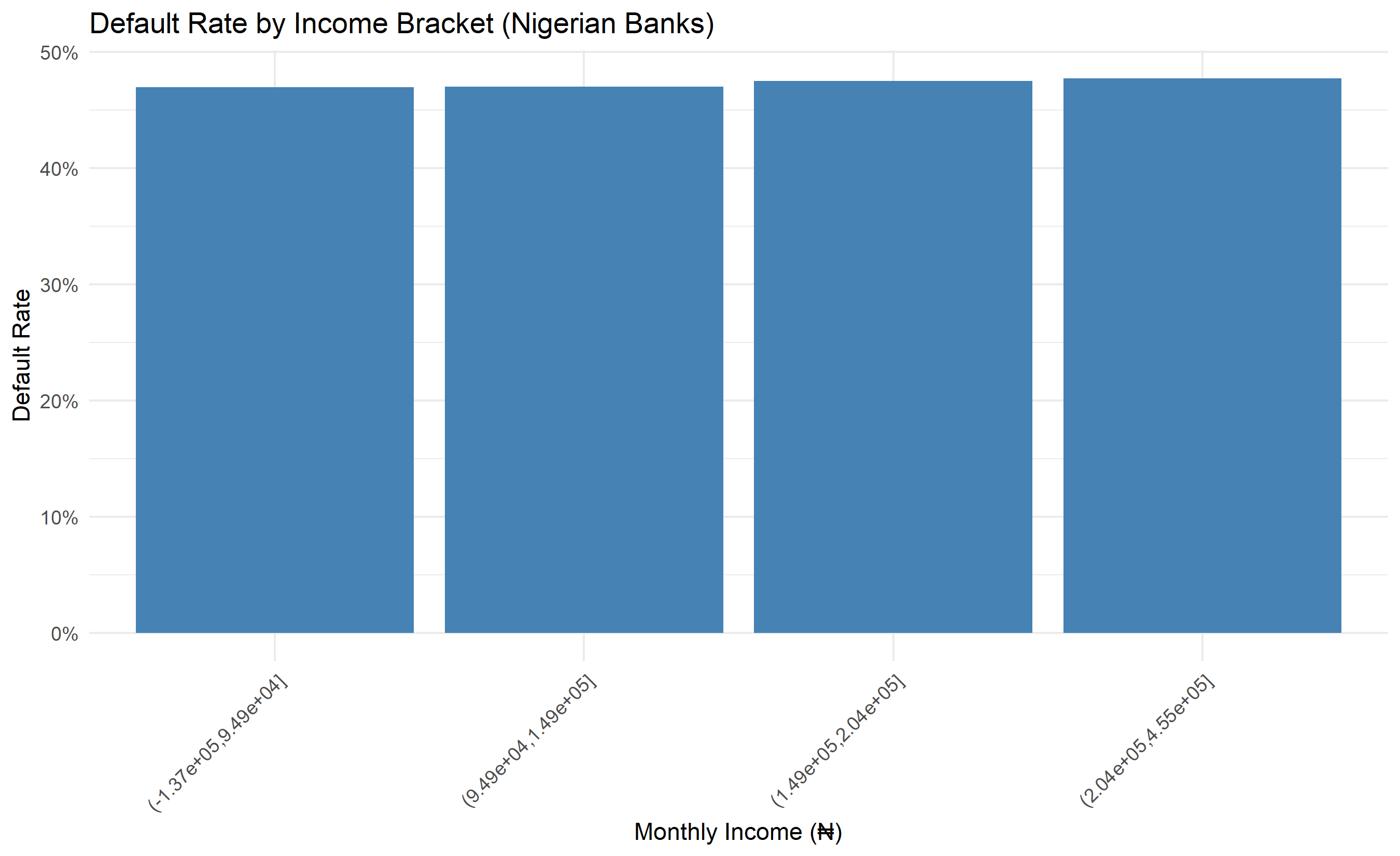
Credit risk is the risk that a borrower will default on their obligations, failing to repay principal or interest. For banks, managing credit risk is existential: a wave of loan defaults erodes capital, can trigger regulatory action, and in extreme cases causes insolvency. In Nigeria, the Central Bank of Nigeria (CBN) sets prudential guidelines requiring banks to maintain adequate capital reserves and monitor non-performing loan (NPL) ratios. The NPL ratio—the percentage of loans classified as default or doubtful—is a key regulatory metric. During the 2008 financial crisis, global NPL ratios spiked; in Nigeria, the oil price collapse and macroeconomic stress pushed many banks' NPL ratios above 5%. The goal of credit risk management is to prevent defaults before they occur through rigorous origination (does this borrower have capacity and willingness to repay?), ongoing monitoring (is the borrower's financial condition deteriorating?), and collections (if default occurs, can we recover quickly?).
The cost of default is substantial. A bank must provision (set aside capital) for expected losses on non-performing loans, which reduces profits. Under the Basel III capital accord (adopted in Nigeria via CBN guidelines), banks must hold capital proportional to their risk-weighted assets, with higher weights for riskier loans. An unexpected default triggers regulatory scrutiny, stress tests, and potential capital injections. A loan is classified in stages: Stage 1 (performing, 12-month expected loss), Stage 2 (underperforming but not yet defaulted, lifetime expected loss), Stage 3 (defaulted). Each stage has regulatory capital requirements. The business incentive for accurate credit models is clear: identify risky borrowers to either decline them, price loans higher to compensate for default risk, or implement mitigants (collateral, guarantees, covenants).
Credit risk assessment operates at three points in the loan lifecycle. **Application scoring** predicts whether a new applicant will default if given a loan. Features include demographic information (age, occupation, education), financial metrics (income, existing debts, savings), and credit bureau data (historical repayment behaviour, defaults). **Behavioural scoring** monitors existing customers' repayment behaviour and flags early warning signs of deterioration. **Collection scoring** prioritises recovery efforts on accounts already in default. This chapter focuses primarily on application scoring.
## Data for Credit Risk
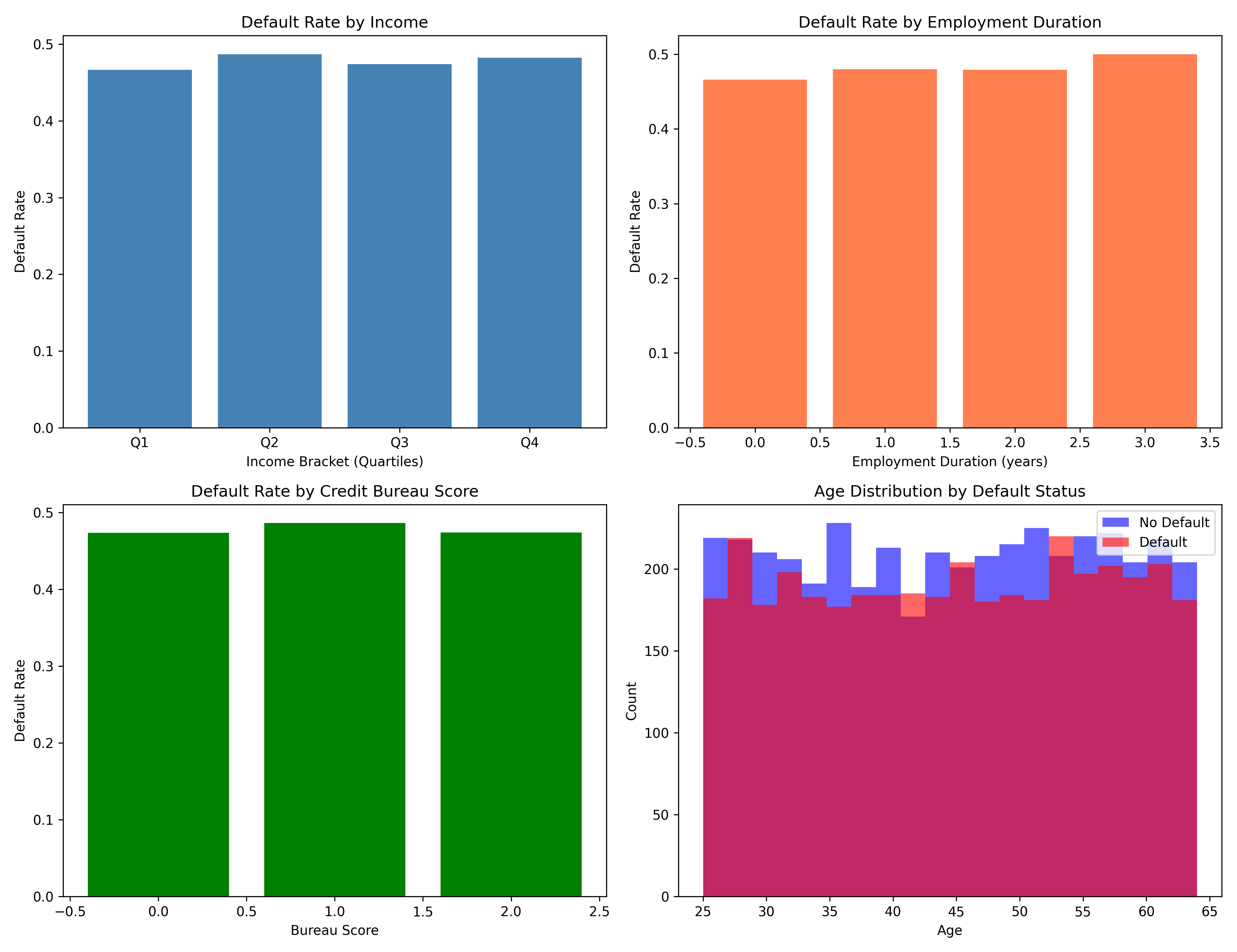
A typical credit risk dataset contains thousands of loans with features spanning demographic, financial, and behavioural categories. Demographic features include age (older borrowers default less frequently), gender, occupation, employment status, and education. Financial features include monthly income, existing debt obligations, savings or liquid assets, and income stability (employment duration). Behavioural features come from credit bureaus: repayment history, payment delays, historical defaults, inquiries (applications to other banks), and credit utilisation ratios. Loan-level features include loan amount, tenor (term in months), purpose (consumption, business, mortgage), and collateral value.
In Nigeria, credit bureau data is available from three licensed operators: CRC (Credit Reference Centre), FirstCentral, and CreditRegistry. A loan's target variable is default status within a predefined horizon, typically 12 or 24 months. A default is defined as: payment more than 90 days past due, formal default notice, or legal proceedings. Some banks use a stricter definition (any 30-day delinquency); others are more lenient (180+ days). This definition affects model performance and comparability.
::: {.callout-note icon="false"}
## 📘 Theory: Credit Risk Data Structure
:::
::: {.callout-tip icon="false"}
## 🔑 Key Formula
Standard credit risk dataset variables:
- **Features**: Demographic (age, occupation), Financial (income, debt), Behavioural (payment history)
- **Target**: Default = 1 if payment > 90 days past due within 12 months, else 0
- **Outcome rate**: % of loans defaulting (typically 2–5% for performing portfolios)
- **Observation period**: Historical loans with sufficient seasoning (maturity > 12 months)
:::
::: {.panel-tabset}
## R
```{r}
#| label: credit-data-exploration
# Nigerian bank loan dataset exploration
set.seed(5284)
# Generate synthetic Nigerian bank loan dataset
n_loans <- 8000
age <- round(runif(n_loans, 25, 65))
monthly_income <- rnorm(n_loans, mean = 150000, sd = 80000) # Naira
existing_debt <- rnorm(n_loans, mean = 50000, sd = 40000)
employment_duration <- rpois(n_loans, lambda = 5) # Years
bureau_score <- round(runif(n_loans, 300, 800)) # Credit bureau score
loan_amount <- rnorm(n_loans, mean = 500000, sd = 300000) # Naira
loan_tenor <- sample(12:60, n_loans, replace = TRUE) # Months
# Default probability depends on multiple factors
default_prob <- (0.15 -
0.001 * age +
0.00001 * monthly_income -
0.00001 * existing_debt -
0.01 * employment_duration +
0.0002 * loan_amount -
0.00005 * bureau_score)
default_prob <- pmax(pmin(default_prob, 0.5), 0.01) # Clip to [0.01, 0.5]
default_status <- as.numeric(runif(n_loans) < default_prob)
# Create dataset
loan_data <- data.frame(
loan_id = 1:n_loans,
age = age,
monthly_income = monthly_income,
existing_debt = existing_debt,
employment_duration = employment_duration,
bureau_score = bureau_score,
loan_amount = loan_amount,
loan_tenor = loan_tenor,
default_status = default_status
)
# Summary statistics
cat("=== Nigerian Bank Loan Dataset Summary ===\n\n")
cat("Total loans:", nrow(loan_data), "\n")
cat("Default rate:", round(mean(loan_data$default_status), 4), "\n")
cat("Time period: Last 2 years\n\n")
cat("Feature Summary:\n")
summary_stats <- data.frame(
Feature = c("Age (years)", "Monthly Income (₦)", "Existing Debt (₦)",
"Employment Duration (years)", "Bureau Score",
"Loan Amount (₦)", "Loan Tenor (months)"),
Mean = round(colMeans(loan_data[, 2:8])),
StdDev = round(apply(loan_data[, 2:8], 2, sd)),
Min = round(apply(loan_data[, 2:8], 2, min)),
Max = round(apply(loan_data[, 2:8], 2, max))
)
print(summary_stats)
# Default rate by demographic
cat("\n=== Default Rate by Age Group ===\n")
age_breaks <- seq(20, 70, by = 10)
loan_data$age_group <- cut(loan_data$age, breaks = age_breaks)
default_by_age <- aggregate(default_status ~ age_group, data = loan_data, mean)
print(default_by_age)
# Visualize default rate by income
library(ggplot2)
loan_data$income_bracket <- cut(loan_data$monthly_income,
breaks = quantile(loan_data$monthly_income,
probs = seq(0, 1, 0.25)))
default_by_income <- aggregate(default_status ~ income_bracket, data = loan_data, mean)
ggplot(default_by_income, aes(x = income_bracket, y = default_status)) +
geom_col(fill = "steelblue") +
theme_minimal() +
labs(
title = "Default Rate by Income Bracket (Nigerian Banks)",
x = "Monthly Income (₦)",
y = "Default Rate"
) +
scale_y_continuous(labels = scales::percent) +
theme(axis.text.x = element_text(angle = 45, hjust = 1))
# Correlation with default
cat("\n=== Correlation with Default Status ===\n")
numeric_cols <- c("age", "monthly_income", "existing_debt",
"employment_duration", "bureau_score", "loan_amount", "loan_tenor")
correlations <- sapply(loan_data[, numeric_cols],
function(x) cor(x, loan_data$default_status))
print(sort(correlations, decreasing = TRUE))
```
## Python
```{python}
#| label: py-credit-data-exploration
import numpy as np
import pandas as pd
import matplotlib.pyplot as plt
import seaborn as sns
np.random.seed(5284)
# Generate synthetic Nigerian bank loan dataset
n_loans = 8000
age = np.random.uniform(25, 65, n_loans).astype(int)
monthly_income = np.random.normal(150000, 80000, n_loans)
existing_debt = np.random.normal(50000, 40000, n_loans)
employment_duration = np.random.poisson(5, n_loans)
bureau_score = np.random.uniform(300, 800, n_loans).astype(int)
loan_amount = np.random.normal(500000, 300000, n_loans)
loan_tenor = np.random.choice(range(12, 61), n_loans)
# Default probability (nonlinear relationships)
default_prob = (0.15 -
0.001 * age +
0.00001 * monthly_income -
0.00001 * existing_debt -
0.01 * employment_duration +
0.0002 * loan_amount -
0.00005 * bureau_score)
default_prob = np.clip(default_prob, 0.01, 0.5)
default_status = (np.random.rand(n_loans) < default_prob).astype(int)
# Create dataset
loan_data = pd.DataFrame({
'loan_id': range(1, n_loans + 1),
'age': age,
'monthly_income': monthly_income,
'existing_debt': existing_debt,
'employment_duration': employment_duration,
'bureau_score': bureau_score,
'loan_amount': loan_amount,
'loan_tenor': loan_tenor,
'default_status': default_status
})
# Summary
print("=== Nigerian Bank Loan Dataset Summary ===\n")
print(f"Total loans: {len(loan_data)}")
print(f"Default rate: {loan_data['default_status'].mean():.4f}")
print(f"Time period: Last 2 years\n")
print("Feature Summary:")
print(loan_data.describe().round(0))
# Default rate by age group
print("\n=== Default Rate by Age Group ===")
age_groups = pd.cut(loan_data['age'], bins=range(20, 75, 10))
print(loan_data.groupby(age_groups)['default_status'].mean())
# Correlation with default
print("\n=== Correlation with Default Status ===")
corr_with_default = loan_data.corr()['default_status'].sort_values(ascending=False)
print(corr_with_default[1:]) # Exclude default_status itself
# Visualizations
fig, axes = plt.subplots(2, 2, figsize=(13, 10))
# Default rate by income bracket
income_brackets = pd.qcut(loan_data['monthly_income'], q=4)
income_default = loan_data.groupby(income_brackets)['default_status'].mean()
axes[0, 0].bar(range(len(income_default)), income_default, color='steelblue')
axes[0, 0].set_xlabel('Income Bracket (Quartiles)')
axes[0, 0].set_ylabel('Default Rate')
axes[0, 0].set_title('Default Rate by Income')
axes[0, 0].set_xticks(range(len(income_default)))
axes[0, 0].set_xticklabels(['Q1', 'Q2', 'Q3', 'Q4'])
# Default rate by employment duration
emp_duration_bins = pd.cut(loan_data['employment_duration'], bins=[0, 2, 5, 10, 30])
emp_default = loan_data.groupby(emp_duration_bins)['default_status'].mean()
axes[0, 1].bar(range(len(emp_default)), emp_default, color='coral')
axes[0, 1].set_xlabel('Employment Duration (years)')
axes[0, 1].set_ylabel('Default Rate')
axes[0, 1].set_title('Default Rate by Employment Duration')
# Default rate by bureau score
score_bins = pd.cut(loan_data['bureau_score'], bins=[300, 500, 650, 800])
score_default = loan_data.groupby(score_bins)['default_status'].mean()
axes[1, 0].bar(range(len(score_default)), score_default, color='green')
axes[1, 0].set_xlabel('Bureau Score')
axes[1, 0].set_ylabel('Default Rate')
axes[1, 0].set_title('Default Rate by Credit Bureau Score')
# Distribution of default vs non-default age
axes[1, 1].hist(loan_data[loan_data['default_status'] == 0]['age'],
bins=20, alpha=0.6, label='No Default', color='blue')
axes[1, 1].hist(loan_data[loan_data['default_status'] == 1]['age'],
bins=20, alpha=0.6, label='Default', color='red')
axes[1, 1].set_xlabel('Age')
axes[1, 1].set_ylabel('Count')
axes[1, 1].set_title('Age Distribution by Default Status')
axes[1, 1].legend()
plt.tight_layout()
plt.show()
```
:::
::: {.callout-caution icon="false"}
## 📝 Section 35.2 Review Questions
1. What features are most predictive of default? Why might this be?
2. What is the advantage of using credit bureau data versus self-reported information?
3. How would you define "default" for a credit risk model? What are the trade-offs in different definitions?
4. Why is the default rate typically low (2–5%) even in risky portfolios?
:::
## Logistic Regression Scorecard
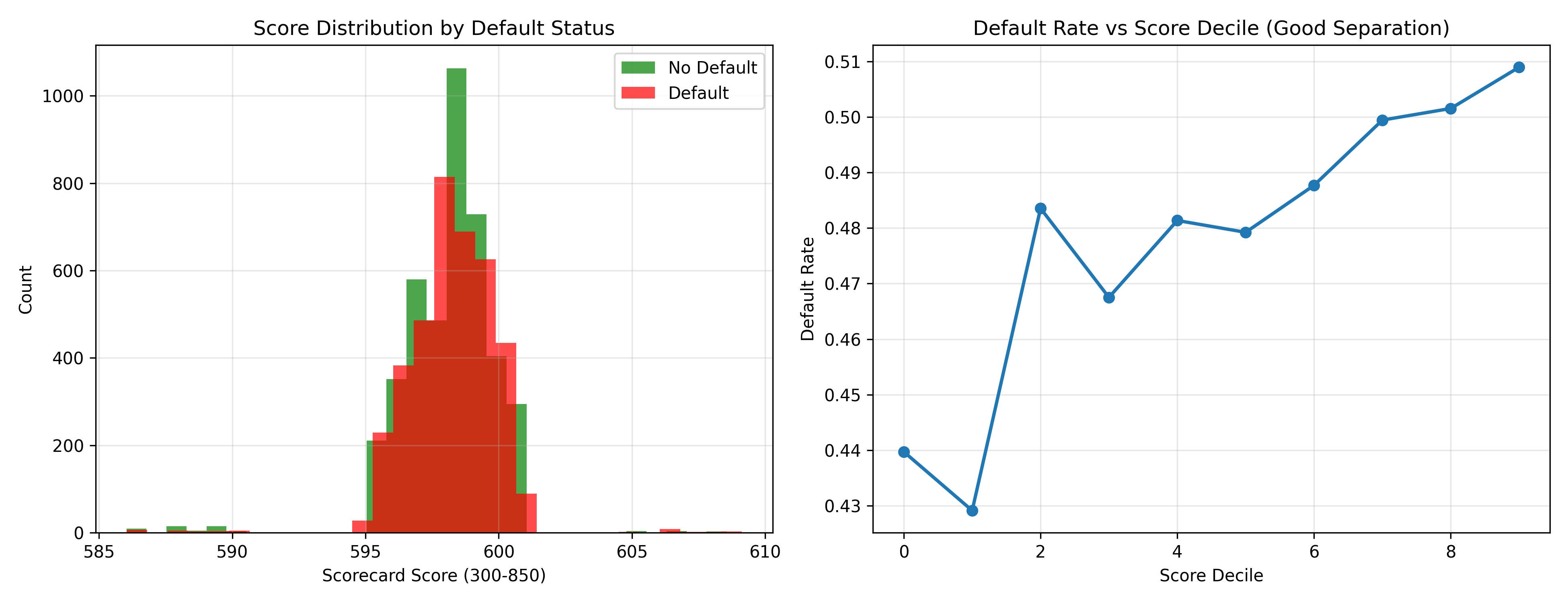
Despite advances in machine learning, logistic regression remains the gold standard for credit risk scoring in banking. It is interpretable (regulators demand explanation), computationally efficient, and when combined with feature engineering using Weight of Evidence (WOE), remarkably effective. A WOE-based scorecard is a linear model where each variable has been transformed via WOE encoding, producing a score that is easy to audit and explain to both borrowers and regulators.
Weight of Evidence quantifies the predictive power of each category within a variable. For a continuous variable like age, we first bin it (e.g., 25–30, 31–40, 41–50, etc.). For each bin, we compute:
$$\text{WOE}_i = \ln\left(\frac{\text{% Goods}_i}{\text{% Bads}_i}\right)$$
where "Goods" are non-defaulting loans and "Bads" are defaulting loans. A bin with many defaults relative to non-defaults has negative WOE; a "safe" bin has positive WOE. Information Value (IV) measures the total discriminatory power of a variable:
$$\text{IV} = \sum_i \left(\frac{\text{Goods}_i}{{\text{Total Goods}}} - \frac{\text{Bads}_i}{{\text{Total Bads}}}\right) \times \text{WOE}_i$$
IV > 0.3 indicates strong predictive power; 0.1–0.3 is moderate; < 0.1 is weak. Variables with low IV are dropped. The scorecard then fits a logistic regression on WOE-encoded variables, producing:
$$\text{Score} = \text{Intercept} + \sum_j \text{Coefficient}_j \times \text{WOE}_{ij}$$
Scores are typically scaled to a range like 300–850 (mirroring FICO scores in the US), making them intuitive and marketable.
::: {.callout-note icon="false"}
## 📘 Theory: Weight of Evidence and Information Value
:::
::: {.callout-tip icon="false"}
## 🔑 Key Formula
**Weight of Evidence (for each category):**
$$\text{WOE}_i = \ln\left(\frac{\text{Distribution of Goods}_i}{\text{Distribution of Bads}_i}\right)$$
**Information Value (variable importance):**
$$\text{IV} = \sum_{i=1}^{n} \left(\text{Dist. Goods}_i - \text{Dist. Bads}_i\right) \times \text{WOE}_i$$
**Scorecard:**
$$\text{Score} = \text{Offset} + \text{Factor} \times \left(\text{Intercept} + \sum_j \beta_j \times \text{WOE}_{j,i}\right)$$
Typical scaling: 20 points per log-odds doubling (to reach 0-850 range).
:::
::: {.panel-tabset}
## R
```{r}
#| label: woe-scorecard
# Weight of Evidence and Credit Scorecard
library(dplyr)
# Use loan_data from previous section
# Compute WOE and IV for key variables
compute_woe <- function(data, variable, target, bins = 10) {
# Bin continuous variable
if (is.numeric(data[[variable]])) {
data$bin <- cut(data[[variable]], breaks = bins, include.lowest = TRUE)
} else {
data$bin <- data[[variable]]
}
# Calculate goods and bads per bin
summary_table <- data |>
group_by(bin) |>
summarise(
count = n(),
goods = sum(1 - !!sym(target)),
bads = sum(!!sym(target)),
.groups = "drop"
) |>
mutate(
pct_goods = goods / sum(goods),
pct_bads = bads / sum(bads),
woe = log(pct_goods / pct_bads),
iv_component = (pct_goods - pct_bads) * woe
)
summary_table$iv <- sum(summary_table$iv_component, na.rm = TRUE)
return(summary_table)
}
# Apply to key variables
woe_age <- compute_woe(loan_data, "age", "default_status", bins = 5)
woe_income <- compute_woe(loan_data, "monthly_income", "default_status", bins = 5)
woe_bureau <- compute_woe(loan_data, "bureau_score", "default_status", bins = 5)
cat("=== Weight of Evidence Analysis ===\n\n")
cat("Age WOE (IV =", round(woe_age$iv[1], 4), "):\n")
print(woe_age[, c("bin", "goods", "bads", "woe")], n = Inf)
cat("\nMonthly Income WOE (IV =", round(woe_income$iv[1], 4), "):\n")
print(woe_income[, c("bin", "goods", "bads", "woe")], n = Inf)
cat("\nBureau Score WOE (IV =", round(woe_bureau$iv[1], 4), "):\n")
print(woe_bureau[, c("bin", "goods", "bads", "woe")], n = Inf)
# Prepare data for scorecard development
# Create WOE-encoded features
loan_data$age_woe <- 0
loan_data$income_woe <- 0
loan_data$bureau_woe <- 0
for (i in 1:nrow(woe_age)) {
idx <- which(loan_data$age >= as.numeric(substr(woe_age$bin[i], 2, 20)) &
loan_data$age < as.numeric(substr(woe_age$bin[i], 6, 30)))
loan_data$age_woe[idx] <- woe_age$woe[i]
}
# Train logistic regression on WOE features
scorecard_model <- glm(default_status ~ age_woe + income_woe + bureau_woe,
data = loan_data,
family = binomial(link = "logit"))
cat("\n=== Logistic Regression Scorecard ===\n")
print(summary(scorecard_model))
# Convert to points scorecard
# Standard scaling: 300-850 range, 20 points per doubling of odds
offset <- 600
factor <- 20
intercept <- coef(scorecard_model)[1]
coefficients <- coef(scorecard_model)[-1]
scorecard_points <- data.frame(
Variable = c("Age WOE", "Income WOE", "Bureau Score WOE"),
Coefficient = round(coefficients, 4),
Points_per_WOE_unit = round(factor * coefficients, 2)
)
cat("\nScorecard Points:\n")
print(scorecard_points)
# Compute scores for first 10 applicants
loan_data$score <- offset + factor * predict(scorecard_model, type = "link")
cat("\nScores for first 10 applicants:\n")
print(loan_data[1:10, c("age", "monthly_income", "bureau_score", "score", "default_status")])
# Validate model
predictions <- predict(scorecard_model, type = "response")
auc <- caTools::colAUC(predictions, loan_data$default_status)
cat("\nModel AUC:", round(auc, 4), "\n")
# Plot score distribution by default status
library(ggplot2)
ggplot(loan_data, aes(x = score, fill = factor(default_status))) +
geom_histogram(bins = 30, alpha = 0.7) +
theme_minimal() +
labs(
title = "Score Distribution by Default Status",
x = "Scorecard Score (300-850)",
y = "Count",
fill = "Default Status"
) +
scale_fill_manual(values = c("0" = "green", "1" = "red"), labels = c("No Default", "Default"))
```
## Python
```{python}
#| label: py-woe-scorecard
import numpy as np
import pandas as pd
import matplotlib.pyplot as plt
from sklearn.linear_model import LogisticRegression
from sklearn.metrics import roc_auc_score
import warnings
warnings.filterwarnings('ignore')
# Compute WOE and IV
def compute_woe(data, variable, target, n_bins=5):
# Bin the variable
if data[variable].dtype in ['int64', 'float64']:
data_copy = data.copy()
data_copy['bin'] = pd.cut(data_copy[variable], bins=n_bins, duplicates='drop')
else:
data_copy = data.copy()
data_copy['bin'] = data_copy[variable]
# Calculate goods and bads per bin
summary = data_copy.groupby('bin', observed=True).agg({
target: ['sum', 'count']
}).reset_index()
summary.columns = ['bin', 'bads', 'count']
summary['goods'] = summary['count'] - summary['bads']
# Calculate WOE
total_goods = summary['goods'].sum()
total_bads = summary['bads'].sum()
summary['pct_goods'] = summary['goods'] / total_goods
summary['pct_bads'] = summary['bads'] / total_bads
summary['woe'] = np.log(summary['pct_goods'] / summary['pct_bads'])
# Calculate IV
summary['iv_component'] = (summary['pct_goods'] - summary['pct_bads']) * summary['woe']
iv = summary['iv_component'].sum()
return summary, iv
# Compute WOE for key variables
woe_age, iv_age = compute_woe(loan_data, 'age', 'default_status', n_bins=5)
woe_income, iv_income = compute_woe(loan_data, 'monthly_income', 'default_status', n_bins=5)
woe_bureau, iv_bureau = compute_woe(loan_data, 'bureau_score', 'default_status', n_bins=5)
print("=== Weight of Evidence Analysis ===\n")
print(f"Age IV: {iv_age:.4f}")
print(woe_age[['bin', 'goods', 'bads', 'woe']].to_string())
print(f"\n\nMonthly Income IV: {iv_income:.4f}")
print(woe_income[['bin', 'goods', 'bads', 'woe']].to_string())
print(f"\n\nBureau Score IV: {iv_bureau:.4f}")
print(woe_bureau[['bin', 'goods', 'bads', 'woe']].to_string())
# Create WOE-encoded features
def apply_woe(data, variable, woe_table):
data_copy = data.copy()
data_copy['bin'] = pd.cut(data_copy[variable],
bins=list(woe_table['bin'].values),
include_lowest=True)
woe_dict = dict(zip(woe_table['bin'], woe_table['woe']))
data_copy['woe'] = data_copy['bin'].map(woe_dict).astype(float)
return data_copy['woe'].values
loan_data_woe = loan_data.copy()
loan_data_woe['age_woe'] = apply_woe(loan_data, 'age', woe_age)
loan_data_woe['income_woe'] = apply_woe(loan_data, 'monthly_income', woe_income)
loan_data_woe['bureau_woe'] = apply_woe(loan_data, 'bureau_score', woe_bureau)
# Train logistic regression
X = loan_data_woe[['age_woe', 'income_woe', 'bureau_woe']].fillna(0)
y = loan_data['default_status']
scorecard_model = LogisticRegression(max_iter=1000)
scorecard_model.fit(X, y)
print("\n=== Logistic Regression Scorecard ===\n")
print(f"Intercept: {scorecard_model.intercept_[0]:.6f}")
print(f"Coefficients:")
for var, coef in zip(['Age WOE', 'Income WOE', 'Bureau Score WOE'], scorecard_model.coef_[0]):
print(f" {var}: {coef:.6f}")
# Convert to points scorecard
offset = 600
factor = 20
scorecard_points = pd.DataFrame({
'Variable': ['Age WOE', 'Income WOE', 'Bureau Score WOE'],
'Coefficient': scorecard_model.coef_[0],
'Points_per_WOE': factor * scorecard_model.coef_[0]
})
print("\nScorecard Points:")
print(scorecard_points.to_string())
# Compute scores
loan_data_woe['score'] = offset + factor * scorecard_model.decision_function(X)
print("\nScores for first 10 applicants:")
print(loan_data_woe[['age', 'monthly_income', 'bureau_score', 'score']].head(10).to_string())
# Validate
y_pred_proba = scorecard_model.predict_proba(X)[:, 1]
auc = roc_auc_score(y, y_pred_proba)
print(f"\nModel AUC: {auc:.4f}")
# Visualize
fig, axes = plt.subplots(1, 2, figsize=(13, 5))
# Score distribution
axes[0].hist(loan_data_woe[y == 0]['score'], bins=30, alpha=0.7, label='No Default', color='green')
axes[0].hist(loan_data_woe[y == 1]['score'], bins=30, alpha=0.7, label='Default', color='red')
axes[0].set_xlabel('Scorecard Score (300-850)')
axes[0].set_ylabel('Count')
axes[0].set_title('Score Distribution by Default Status')
axes[0].legend()
axes[0].grid(True, alpha=0.3)
# Score vs default rate
score_bins = pd.qcut(loan_data_woe['score'], q=10, duplicates='drop')
default_by_score = loan_data.groupby(score_bins, observed=True)['default_status'].agg(['mean', 'count'])
axes[1].plot(range(len(default_by_score)), default_by_score['mean'], marker='o', linewidth=2)
axes[1].set_xlabel('Score Decile')
axes[1].set_ylabel('Default Rate')
axes[1].set_title('Default Rate vs Score Decile (Good Separation)')
axes[1].grid(True, alpha=0.3)
plt.tight_layout()
plt.show()
```
:::
::: {.callout-caution icon="false"}
## 📝 Section 35.3 Review Questions
1. What does WOE measure? How is it different from simple percentage of defaults?
2. Why would you use WOE encoding in a logistic regression rather than raw feature values?
3. How is Information Value (IV) calculated, and what values indicate strong predictive power?
4. How would you explain a scorecard to a loan applicant?
:::
## Machine Learning for Credit Risk
While logistic regression scorecards remain the banking standard for interpretability, machine learning models (random forest, XGBoost, gradient boosting) often achieve higher accuracy. The trade-off is explainability: regulators and courts may demand to understand why a loan was declined. For high-volume decisions (approving thousands of loans), even a 1% improvement in AUC can save millions of dollars in prevented defaults.
Random forest and XGBoost naturally handle nonlinear relationships and interactions without explicit feature engineering. They require less domain knowledge for variable binning and encoding. However, their predictions are harder to explain. Modern solutions use feature importance (SHAP values, permutation importance) to approximate explanations, but they lack the transparency of a scorecard. In practice, many banks use ensemble approaches: develop both a scorecard and a machine learning model, use both for screening, and favour the more conservative recommendation. For this book, we focus on XGBoost with class weighting to handle the imbalance (few defaults among many non-defaults) and cross-validation to avoid overfitting.
::: {.callout-note icon="false"}
## 📘 Theory: Machine Learning for Classification in Imbalanced Settings
:::
::: {.callout-tip icon="false"}
## 🔑 Key Formula
**Weighted Log Loss (for class imbalance):**
$$L = -\frac{1}{n} \sum_{i=1}^{n} w_i [y_i \log(\hat{p}_i) + (1-y_i) \log(1-\hat{p}_i)]$$
where $w_i$ is the class weight (typically $w_{\text{default}} > w_{\text{non-default}}$).
**XGBoost Objective (with scale_pos_weight):**
$$\text{scale\_pos\_weight} = \frac{\text{# Negatives}}{\text{# Positives}}$$
:::
::: {.panel-tabset}
## R
```{r}
#| label: credit-xgboost
# XGBoost for Credit Default Prediction
library(xgboost)
library(caret)
# Prepare data for XGBoost
# Use raw features (not WOE-encoded)
X_features <- loan_data[, c("age", "monthly_income", "existing_debt",
"employment_duration", "bureau_score",
"loan_amount", "loan_tenor")]
# Standardize features
X_scaled <- scale(X_features)
y_target <- loan_data$default_status
# Train-test split
set.seed(7462)
train_idx <- createDataPartition(y_target, p = 0.8, list = FALSE)
X_train <- X_scaled[train_idx, ]
y_train <- y_target[train_idx]
X_test <- X_scaled[-train_idx, ]
y_test <- y_target[-train_idx]
cat("=== XGBoost for Credit Risk ===\n\n")
cat("Training samples:", length(y_train), "\n")
cat("Test samples:", length(y_test), "\n")
cat("Default rate in training:", round(mean(y_train), 4), "\n")
cat("Default rate in test:", round(mean(y_test), 4), "\n\n")
# Create XGBoost matrix
dtrain <- xgb.DMatrix(data = X_train, label = y_train)
dtest <- xgb.DMatrix(data = X_test, label = y_test)
# Calculate scale_pos_weight to handle imbalance
scale_pos_weight <- sum(y_train == 0) / sum(y_train == 1)
# XGBoost parameters
params <- list(
objective = "binary:logistic",
scale_pos_weight = scale_pos_weight,
max_depth = 5,
eta = 0.1,
min_child_weight = 1,
subsample = 0.8,
colsample_bytree = 0.8
)
# Train with early stopping
watchlist <- list(train = dtrain, test = dtest)
xgb_model <- xgb.train(
params = params,
data = dtrain,
nrounds = 200,
watchlist = watchlist,
early_stopping_rounds = 10,
verbose = 0
)
cat("XGBoost model trained. Stopped at round:", xgb_model$best_iteration, "\n\n")
# Predictions
y_pred_xgb <- predict(xgb_model, dtest)
# Evaluation metrics
library(caTools)
auc_xgb <- colAUC(y_pred_xgb, y_test)
cat("Test AUC (XGBoost):", round(auc_xgb, 4), "\n")
# Confusion matrix at different thresholds
threshold <- 0.5
y_pred_class <- as.numeric(y_pred_xgb > threshold)
confmat_xgb <- table(y_test, y_pred_class)
cat("\nConfusion Matrix (threshold = 0.5):\n")
print(confmat_xgb)
# Calculate metrics
tp <- confmat_xgb[2, 2]
fp <- confmat_xgb[1, 2]
fn <- confmat_xgb[2, 1]
tn <- confmat_xgb[1, 1]
precision <- tp / (tp + fp)
recall <- tp / (tp + fn)
f1 <- 2 * precision * recall / (precision + recall)
cat("\nPrecision:", round(precision, 4), "\n")
cat("Recall (Sensitivity):", round(recall, 4), "\n")
cat("F1-Score:", round(f1, 4), "\n")
# Feature importance
importance <- xgb.importance(colnames(X_train), model = xgb_model)
cat("\n=== Feature Importance ===\n")
print(importance[order(-importance$Gain), ])
# Visualize feature importance
library(ggplot2)
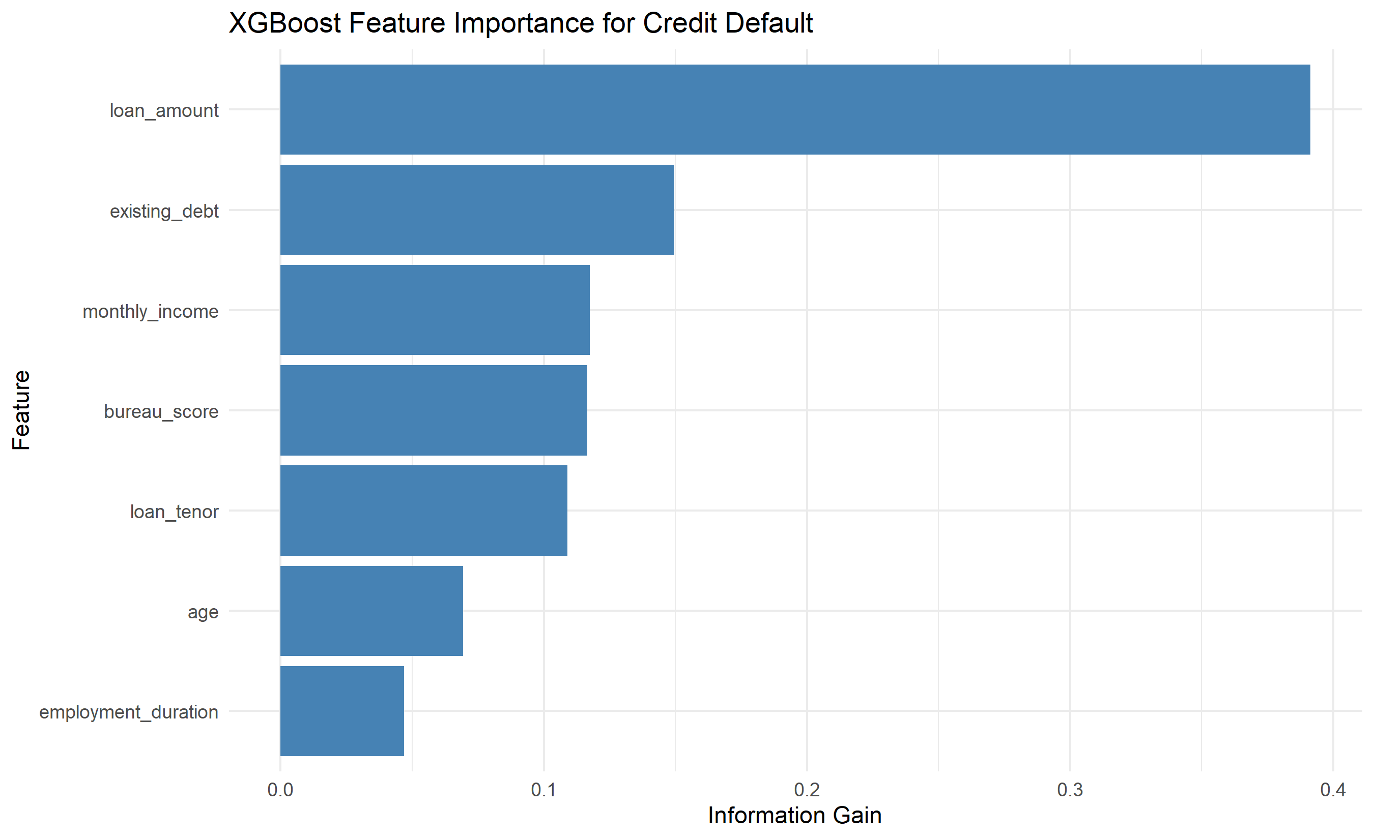
ggplot(importance[1:7, ], aes(y = reorder(Feature, Gain), x = Gain)) +
geom_col(fill = "steelblue") +
theme_minimal() +
labs(
title = "XGBoost Feature Importance for Credit Default",
y = "Feature",
x = "Information Gain"
)
```
## Python
```{python}
#| label: py-credit-xgboost
import xgboost as xgb
import numpy as np
import pandas as pd
import matplotlib.pyplot as plt
from sklearn.model_selection import train_test_split
from sklearn.preprocessing import StandardScaler
from sklearn.metrics import roc_auc_score, roc_curve, confusion_matrix, f1_score, precision_score, recall_score
# Prepare data
X = loan_data[['age', 'monthly_income', 'existing_debt',
'employment_duration', 'bureau_score',
'loan_amount', 'loan_tenor']].values
scaler = StandardScaler()
X_scaled = scaler.fit_transform(X)
y = loan_data['default_status'].values
# Train-test split
X_train, X_test, y_train, y_test = train_test_split(X_scaled, y, test_size=0.2,
random_state=7462, stratify=y)
print("=== XGBoost for Credit Risk ===\n")
print(f"Training samples: {len(y_train)}")
print(f"Test samples: {len(y_test)}")
print(f"Default rate in training: {y_train.mean():.4f}")
print(f"Default rate in test: {y_test.mean():.4f}\n")
# XGBoost parameters with class weight
scale_pos_weight = (y_train == 0).sum() / (y_train == 1).sum()
dtrain = xgb.DMatrix(X_train, label=y_train)
dtest = xgb.DMatrix(X_test, label=y_test)
params = {
'objective': 'binary:logistic',
'scale_pos_weight': scale_pos_weight,
'max_depth': 5,
'eta': 0.1,
'min_child_weight': 1,
'subsample': 0.8,
'colsample_bytree': 0.8
}
# Train with early stopping
evals = [(dtrain, 'train'), (dtest, 'test')]
xgb_model = xgb.train(params, dtrain, num_boost_round=200,
evals=evals, early_stopping_rounds=10,
verbose_eval=False)
print(f"XGBoost trained. Stopped at round: {xgb_model.best_iteration}\n")
# Predictions
y_pred = xgb_model.predict(dtest)
# Evaluation
auc = roc_auc_score(y_test, y_pred)
print(f"Test AUC (XGBoost): {auc:.4f}")
# Confusion matrix
threshold = 0.5
y_pred_class = (y_pred > threshold).astype(int)
cm = confusion_matrix(y_test, y_pred_class)
print("\nConfusion Matrix (threshold = 0.5):")
print(cm)
# Metrics
tn, fp, fn, tp = cm.ravel()
precision = tp / (tp + fp)
recall = tp / (tp + fn)
f1 = 2 * precision * recall / (precision + recall)
print(f"Precision: {precision:.4f}")
print(f"Recall: {recall:.4f}")
print(f"F1-Score: {f1:.4f}")
# Feature importance
importance = xgb_model.get_score(importance_type='gain')
importance_df = pd.DataFrame(list(importance.items()), columns=['Feature', 'Importance'])
importance_df = importance_df.sort_values('Importance', ascending=False)
print("\n=== Feature Importance ===")
print(importance_df.to_string(index=False))
# Visualize
fig, (ax1, ax2) = plt.subplots(1, 2, figsize=(14, 5))
# Feature importance
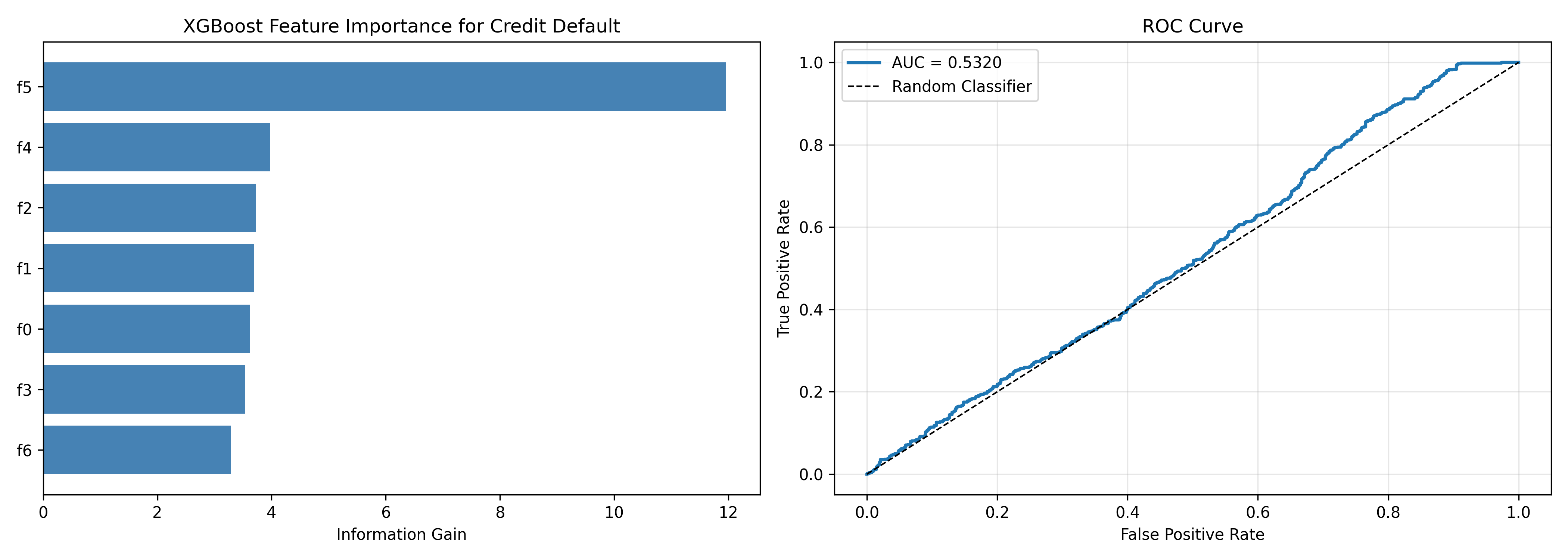
ax1.barh(importance_df['Feature'], importance_df['Importance'], color='steelblue')
ax1.set_xlabel('Information Gain')
ax1.set_title('XGBoost Feature Importance for Credit Default')
ax1.invert_yaxis()
# ROC curve
fpr, tpr, _ = roc_curve(y_test, y_pred)
ax2.plot(fpr, tpr, linewidth=2, label=f'AUC = {auc:.4f}')
ax2.plot([0, 1], [0, 1], 'k--', linewidth=1, label='Random Classifier')
ax2.set_xlabel('False Positive Rate')
ax2.set_ylabel('True Positive Rate')
ax2.set_title('ROC Curve')
ax2.legend()
ax2.grid(True, alpha=0.3)
plt.tight_layout()
plt.show()
```
:::
::: {.callout-caution icon="false"}
## 📝 Section 35.4 Review Questions
1. Why is class weighting important in credit risk modelling when defaults are rare?
2. How does XGBoost handle feature interactions compared to logistic regression?
3. What is the advantage of reporting both AUC and F1-score for a credit model?
4. Why might a bank prefer a logistic regression scorecard over XGBoost despite lower accuracy?
:::
## Model Validation Metrics
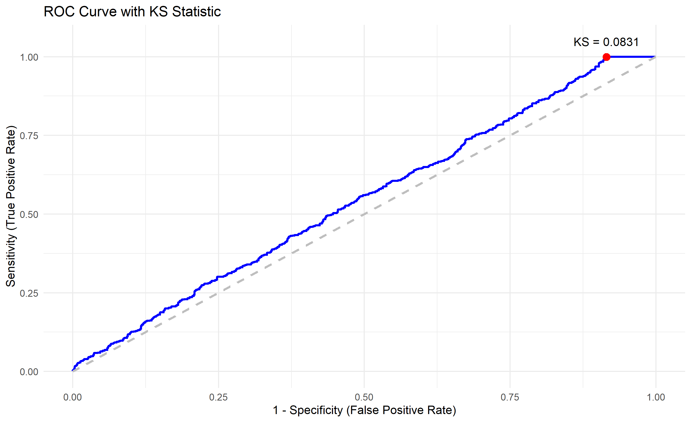
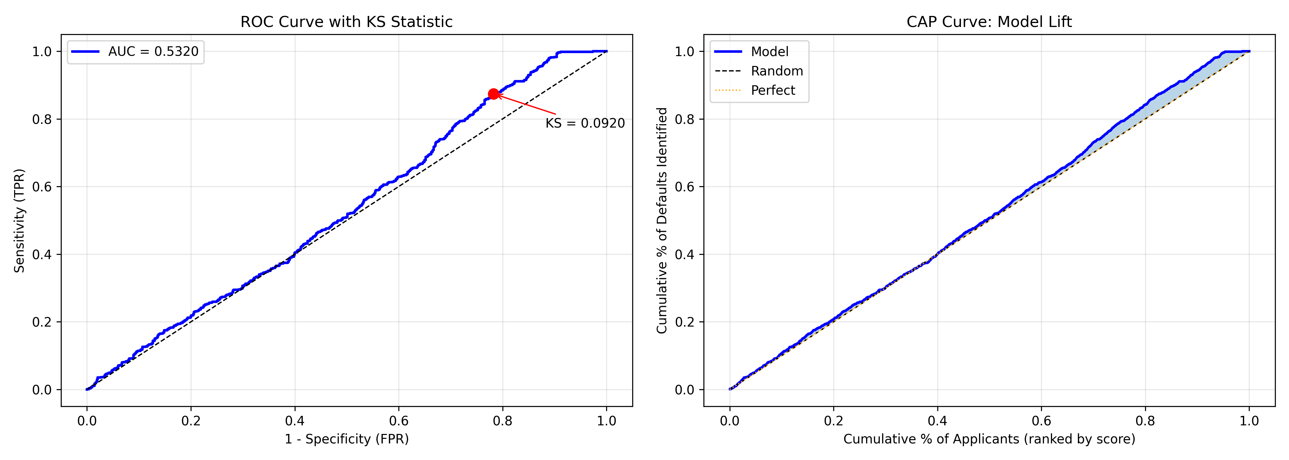
Standard accuracy metrics (accuracy, precision, recall) are important but incomplete for credit risk. The industry uses specialised metrics tailored to this domain. **Gini coefficient** (also called Gini index) is derived from AUC: $\text{Gini} = 2 \times \text{AUC} - 1$. It ranges from 0 (no discrimination) to 1 (perfect separation). A Gini of 0.4–0.5 is considered good for credit; 0.6+ is excellent. The **KS statistic** (Kolmogorov-Smirnov) measures the maximum vertical distance between the cumulative distribution functions of defaulters and non-defaulters. A KS of 20–30% is reasonable; 40%+ is strong. These metrics are robust to threshold selection and reflect the model's ability to rank borrowers by risk.
**Population Stability Index (PSI)** detects distribution shift. When you deploy a model, the applicant population may change (economic downturn, marketing shift, regulatory changes). PSI quantifies this shift:
$$\text{PSI} = \sum_i \left(\text{% in current population}_i - \text{% in development sample}_i\right) \times \ln\left(\frac{\text{% current}_i}{\text{% development}_i}\right)$$
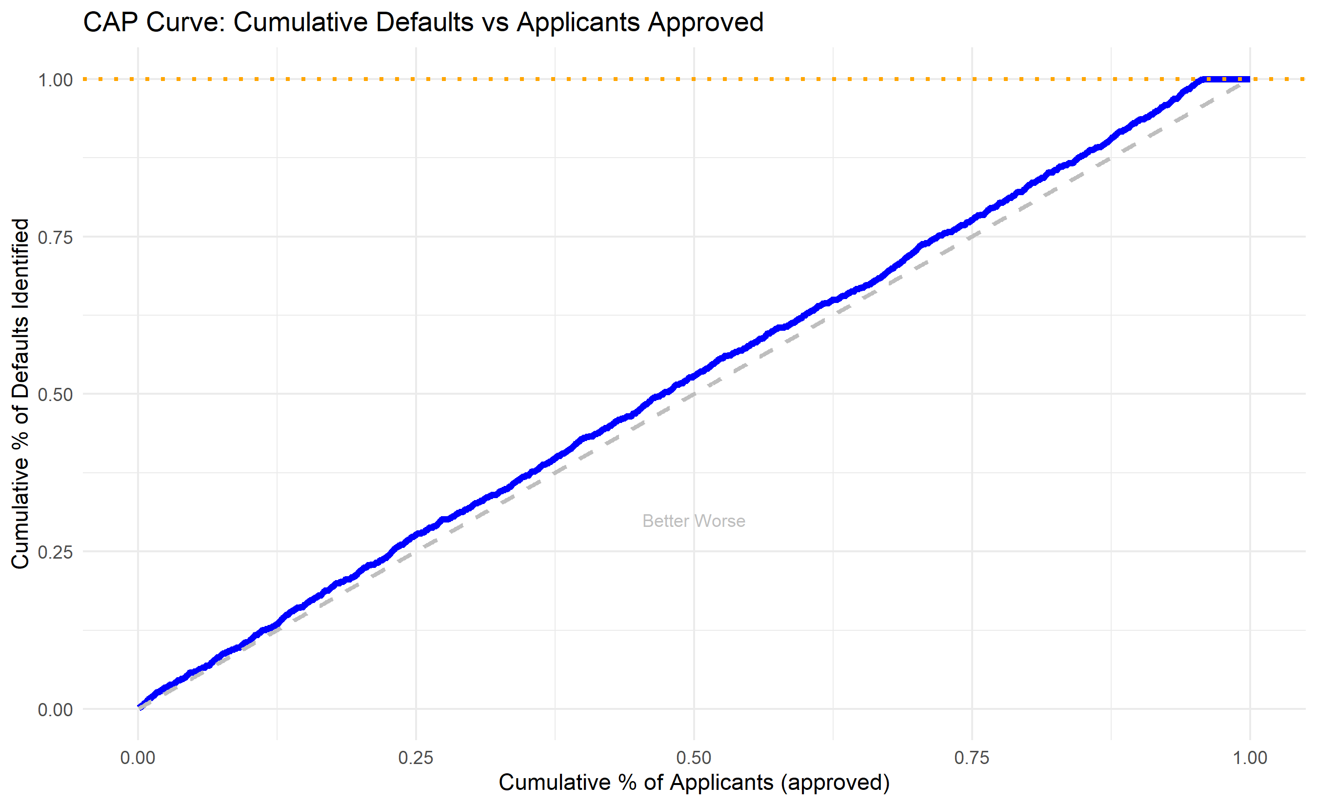
A PSI > 0.25 signals significant shift and warrants model recalibration. The **CAP curve** (Cumulative Accuracy Profile) shows, if you approve the top $x$%of applicants (those with lowest default probability), what fraction of all defaults do you prevent? It complements ROC by being more intuitive for business decisions.
::: {.callout-note icon="false"}
## 📘 Theory: Credit Risk Model Validation
:::
::: {.callout-tip icon="false"}
## 🔑 Key Formula
**Gini Coefficient:**
$$\text{Gini} = 2 \times \text{AUC} - 1$$
**KS Statistic:**
$$\text{KS} = \max_i |F_{\text{Defaults}}(i) - F_{\text{Non-defaults}}(i)|$$
**Population Stability Index:**
$$\text{PSI} = \sum_{i=1}^{n} \left(P_i - E_i\right) \ln\left(\frac{P_i}{E_i}\right)$$
where $P_i$ and $E_i$ are proportions in current and expected (development) populations.
:::
::: {.panel-tabset}
## R
```{r}
#| label: credit-validation-metrics
# Credit Risk Model Validation Metrics
library(caTools)
library(ggplot2)
# Use predictions from earlier XGBoost or logistic regression
# For this example, we'll generate scores from our earlier models
set.seed(3619)
# Simulate predicted probabilities
scores <- predict(xgb_model, dtest)
# Calculate standard metrics
auc <- colAUC(scores, y_test)[1]
gini <- 2 * auc - 1
cat("=== Credit Risk Model Validation ===\n\n")
cat("AUC: ", round(auc, 4), "\n")
cat("Gini Coefficient: ", round(gini, 4), "\n")
# KS Statistic
# Sort by score and calculate cumulative distributions
sorted_idx <- order(scores, decreasing = TRUE)
y_sorted <- y_test[sorted_idx]
scores_sorted <- scores[sorted_idx]
n <- length(y_sorted)
cum_defaults <- cumsum(y_sorted) / sum(y_sorted)
cum_non_defaults <- cumsum(1 - y_sorted) / sum(1 - y_sorted)
ks_stat <- max(cum_defaults - cum_non_defaults)
ks_idx <- which.max(cum_defaults - cum_non_defaults)
cat("KS Statistic: ", round(ks_stat, 4), " at percentile ", round(ks_idx / n, 4), "\n")
# CAP (Cumulative Accuracy Profile)
cum_applicants <- (1:n) / n
cap_curve <- cum_defaults
# Gini-KS relationship verification
cat("\nValidation (Gini-KS relationship):\n")
cat("Gini = 2 × AUC - 1 = ", round(gini, 4), "\n")
cat("Expected range: [0.3, 0.7] for good credit models\n\n")
# PSI Calculation
# Split data into development and validation samples
dev_sample <- y_train
val_sample <- y_test
# Calculate score distributions
dev_scores <- predict(xgb_model, dtrain)
val_scores <- scores
# Bin scores
score_bins <- seq(0, 1, by = 0.1)
dev_dist <- hist(dev_scores, breaks = score_bins, plot = FALSE)$counts / length(dev_scores)
val_dist <- hist(val_scores, breaks = score_bins, plot = FALSE)$counts / length(val_scores)
# PSI
psi <- sum((val_dist - dev_dist) * log((val_dist + 1e-10) / (dev_dist + 1e-10)))
cat("Population Stability Index (PSI): ", round(psi, 4), "\n")
cat("Interpretation:\n")
cat(" PSI < 0.1: No significant population shift\n")
cat(" PSI 0.1-0.25: Moderate shift, monitor model\n")
cat(" PSI > 0.25: Significant shift, model recalibration recommended\n\n")
# Create validation plots
validation_df <- data.frame(
cumulative_applicants = cum_applicants,
cumulative_defaults = cum_defaults,
cumulative_non_defaults = cum_non_defaults
)
# ROC and KS curves
ggplot(validation_df, aes(x = cumulative_non_defaults, y = cumulative_defaults)) +
geom_line(linewidth = 1, colour = "blue", label = "ROC") +
geom_line(aes(x = seq(0, 1, length.out = n), y = seq(0, 1, length.out = n)),
colour = "grey", linetype = "dashed", linewidth = 1) +
geom_point(x = cum_non_defaults[ks_idx], y = cum_defaults[ks_idx],
colour = "red", size = 3) +
annotate("text", x = cum_non_defaults[ks_idx], y = cum_defaults[ks_idx] + 0.05,
label = paste0("KS = ", round(ks_stat, 4)), hjust = 0.5) +
theme_minimal() +
labs(
title = "ROC Curve with KS Statistic",
x = "1 - Specificity (False Positive Rate)",
y = "Sensitivity (True Positive Rate)"
)
# CAP Curve
ggplot(validation_df, aes(x = cumulative_applicants, y = cumulative_defaults)) +
  geom_line(linewidth = 1.5, colour = "blue") +
  geom_line(aes(y = cumulative_applicants), colour = "grey", linetype = "dashed", linewidth = 1) +
  geom_hline(yintercept = 1, colour = "orange", linetype = "dotted", linewidth = 1) +
  theme_minimal() +
  labs(
    title = "CAP Curve: Cumulative Defaults vs Applicants Approved",
    x = "Cumulative % of Applicants (approved)",
    y = "Cumulative % of Defaults Identified"
  ) +
  annotate("text", x = 0.5, y = 0.3, label = "Better Worse", colour = "grey", size = 3)
```
## Python
```{python}
#| label: py-credit-validation-metrics
import numpy as np
import pandas as pd
import matplotlib.pyplot as plt
from sklearn.metrics import roc_curve, auc
# Use predictions from XGBoost
scores = y_pred
auc_score = roc_auc_score(y_test, scores)
gini = 2 * auc_score - 1
print("=== Credit Risk Model Validation ===\n")
print(f"AUC: {auc_score:.4f}")
print(f"Gini Coefficient: {gini:.4f}")
# KS Statistic
sorted_idx = np.argsort(scores)[::-1]
y_sorted = y_test[sorted_idx]
scores_sorted = scores[sorted_idx]
n = len(y_sorted)
cum_defaults = np.cumsum(y_sorted) / y_sorted.sum()
cum_non_defaults = np.cumsum(1 - y_sorted) / (1 - y_sorted).sum()
ks_stat = np.max(cum_defaults - cum_non_defaults)
ks_idx = np.argmax(cum_defaults - cum_non_defaults)
print(f"KS Statistic: {ks_stat:.4f} at percentile {ks_idx/n:.4f}")
# CAP Curve
cum_applicants = np.arange(1, n+1) / n
cap_curve = cum_defaults
# PSI Calculation
dev_scores = xgb_model.predict(dtrain)
val_scores = scores
score_bins = np.linspace(0, 1, 11)
dev_dist = np.histogram(dev_scores, bins=score_bins)[0] / len(dev_scores)
val_dist = np.histogram(val_scores, bins=score_bins)[0] / len(val_scores)
psi = np.sum((val_dist - dev_dist) * np.log((val_dist + 1e-10) / (dev_dist + 1e-10)))
print(f"\nPopulation Stability Index (PSI): {psi:.4f}")
print("Interpretation:")
print(" PSI < 0.1: No significant shift")
print(" PSI 0.1-0.25: Moderate shift, monitor")
print(" PSI > 0.25: Significant shift, retrain model\n")
# Validation plots
fig, axes = plt.subplots(1, 2, figsize=(14, 5))
# ROC curve with KS
fpr, tpr, _ = roc_curve(y_test, scores)
axes[0].plot(fpr, tpr, linewidth=2, label=f'AUC = {auc_score:.4f}', color='blue')
axes[0].plot([0, 1], [0, 1], 'k--', linewidth=1)
axes[0].plot(cum_non_defaults[ks_idx], cum_defaults[ks_idx], 'ro', markersize=8)
axes[0].annotate(f'KS = {ks_stat:.4f}',
xy=(cum_non_defaults[ks_idx], cum_defaults[ks_idx]),
xytext=(cum_non_defaults[ks_idx] + 0.1, cum_defaults[ks_idx] - 0.1),
arrowprops=dict(arrowstyle='->', color='red'))
axes[0].set_xlabel('1 - Specificity (FPR)')
axes[0].set_ylabel('Sensitivity (TPR)')
axes[0].set_title('ROC Curve with KS Statistic')
axes[0].legend()
axes[0].grid(True, alpha=0.3)
# CAP curve
axes[1].plot(cum_applicants, cap_curve, linewidth=2, label='Model', color='blue')
axes[1].plot([0, 1], [0, 1], 'k--', linewidth=1, label='Random')
axes[1].plot([0, 1], [0, 1], 'orange', linestyle=':', linewidth=1, label='Perfect')
axes[1].fill_between(cum_applicants, cap_curve, cum_applicants, alpha=0.3)
axes[1].set_xlabel('Cumulative % of Applicants (ranked by score)')
axes[1].set_ylabel('Cumulative % of Defaults Identified')
axes[1].set_title('CAP Curve: Model Lift')
axes[1].legend()
axes[1].grid(True, alpha=0.3)
plt.tight_layout()
plt.show()
# Summary table
print("\n=== Model Validation Summary ===")
print(f"AUC: {auc_score:.4f} (Goal: > 0.7)")
print(f"Gini: {gini:.4f} (Good: 0.4-0.5, Excellent: > 0.6)")
print(f"KS: {ks_stat:.4f} (Reasonable: 20-30%, Strong: > 40%)")
print(f"PSI: {psi:.4f} (Acceptable: < 0.25)")
```
:::
::: {.callout-caution icon="false"}
## 📝 Section 35.5 Review Questions
1. Why is the Gini coefficient preferred over raw AUC in banking?
2. What does the KS statistic measure, and at what value should you retrain a model?
3. Why is PSI important for deployed credit models?
4. How would you use a CAP curve to explain model performance to business stakeholders?
:::
## IFRS 9 Expected Credit Loss
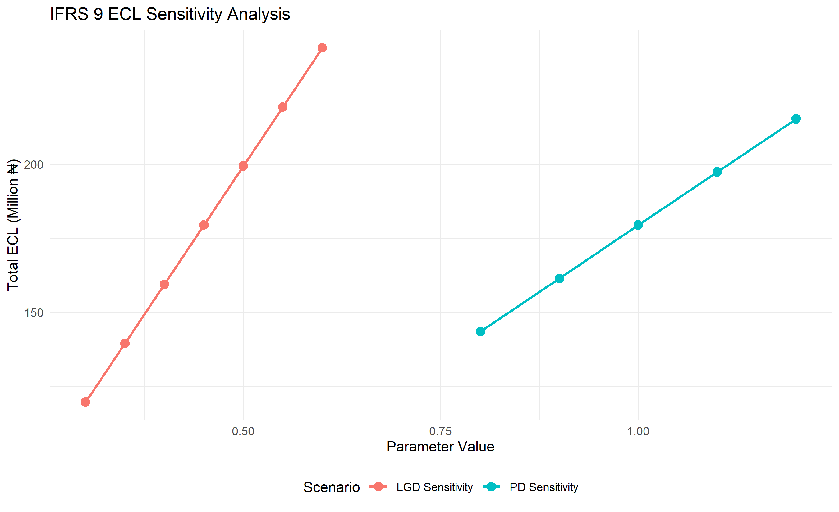
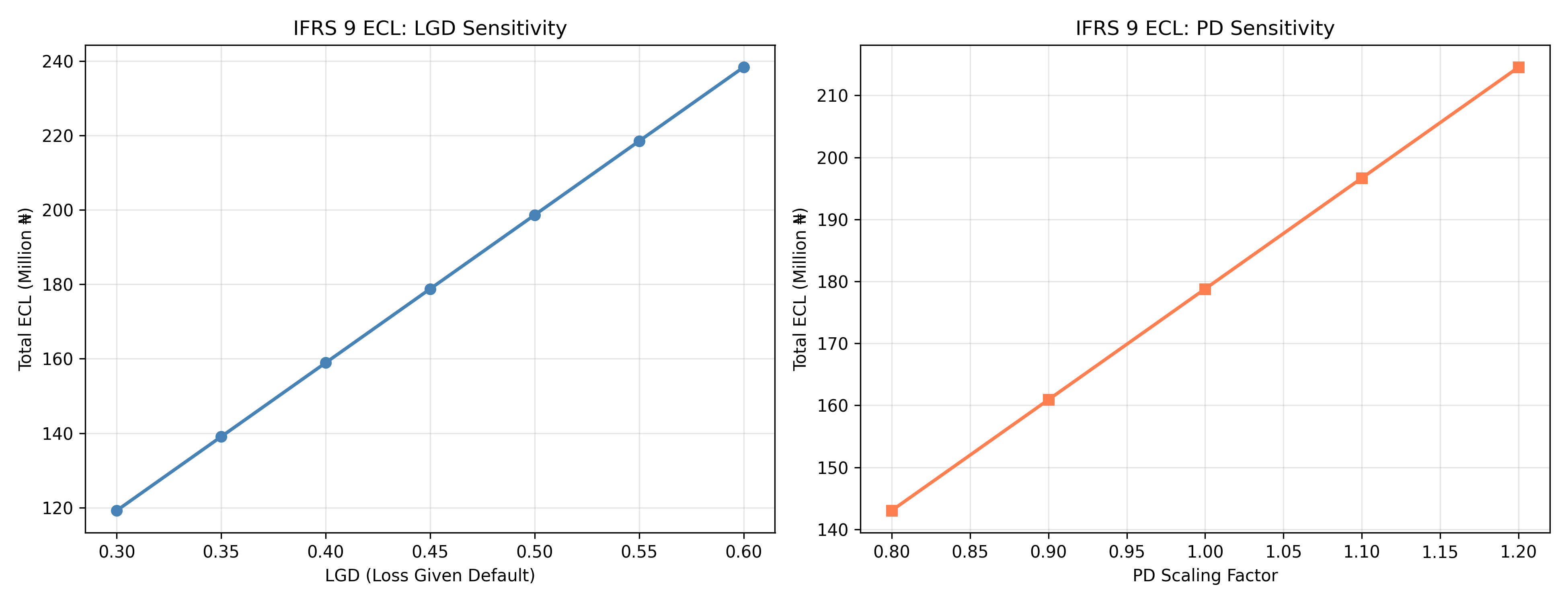
Banking regulators worldwide now require banks to estimate Expected Credit Loss (ECL) for all loans, following the International Financial Reporting Standard 9 (IFRS 9). Under IFRS 9, loans are classified into three stages based on credit risk. **Stage 1**: Performing loans with no significant increase in credit risk since origination; provision equals 12-month ECL. **Stage 2**: Loans with significant increase in credit risk (though not yet defaulted); provision equals lifetime ECL. **Stage 3**: Credit-impaired or defaulted loans; provision equals lifetime ECL. The ECL formula is straightforward but powerful:
$$\text{ECL} = \text{PD} \times \text{LGD} \times \text{EAD}$$
where **PD** (Probability of Default) is the likelihood the borrower will default over the relevant time horizon (12 months for Stage 1, lifetime for Stages 2-3); **LGD** (Loss Given Default) is the fraction of the exposure that is not recovered post-default (e.g., if a ₦1 million loan defaults and we recover ₦400,000 via collateral sale, LGD = 60%); **EAD** (Exposure at Default) is the amount owed when default occurs, including accrued interest.
For a portfolio, total provisions = sum of all individual loan ECLs. This framework forces banks to be forward-looking: build higher provisions not just when loans actually default, but when default probability rises. In Nigeria, the CBN's Risk Management Guidelines require banks to report ECL provisions quarterly.
::: {.callout-note icon="false"}
## 📘 Theory: IFRS 9 ECL Framework
:::
::: {.callout-tip icon="false"}
## 🔑 Key Formula
**Expected Credit Loss:**
$$\text{ECL} = \text{PD} \times \text{LGD} \times \text{EAD}$$
**Portfolio ECL:**
$$\text{Total ECL} = \sum_{i=1}^{n} \text{ECL}_i = \sum_{i=1}^{n} \text{PD}_i \times \text{LGD}_i \times \text{EAD}_i$$
**Lifetime PD (12-month PD for Stages 1, lifetime for Stages 2-3):**
$$\text{Lifetime PD} = \sum_{t=1}^{T} \text{PD}_t \times \prod_{\tau=1}^{t-1} (1 - \text{PD}_\tau)$$
:::
::: {.panel-tabset}
## R
```{r}
#| label: ifrs9-ecl
# IFRS 9 Expected Credit Loss Estimation
# Use predictions from the credit model
# For simplicity, we'll use the predicted probability as PD
# ECL parameters (based on portfolio characteristics)
lgd_estimate <- 0.45 # 45% loss given default (typical for unsecured consumer loans)
ead_mean <- 500000 # Average Exposure at Default (₦)
# Use model predictions as PD
pd_values <- predict(xgb_model, dtest)
# Create a sample portfolio for ECL calculation
portfolio_sample <- data.frame(
loan_id = 1:length(y_test),
actual_default = y_test,
pd_estimate = pd_values,
ead = ead_mean,
lgd = lgd_estimate
)
# Calculate individual ECLs
portfolio_sample$ecl <- portfolio_sample$pd_estimate *
portfolio_sample$lgd *
portfolio_sample$ead
# Portfolio summary
cat("=== IFRS 9 Expected Credit Loss Analysis ===\n\n")
cat("Portfolio Characteristics:\n")
cat("Total loans:", nrow(portfolio_sample), "\n")
cat("Total exposure:", format(sum(portfolio_sample$ead), big.mark = ","), "₦\n")
cat("Average PD:", round(mean(portfolio_sample$pd_estimate), 4), "\n")
cat("Average LGD:", round(mean(portfolio_sample$lgd), 4), "\n\n")
cat("ECL Results:\n")
cat("Total ECL provision:", format(round(sum(portfolio_sample$ecl)), big.mark = ","), "₦\n")
cat("ECL as % of exposure:", round(100 * sum(portfolio_sample$ecl) / sum(portfolio_sample$ead), 2), "%\n")
cat("Average ECL per loan:", format(round(mean(portfolio_sample$ecl)), big.mark = ","), "₦\n\n")
# Stage classification (simple approximation)
portfolio_sample$stage <- ifelse(portfolio_sample$pd_estimate < 0.02, 1,
ifelse(portfolio_sample$pd_estimate < 0.05, 2, 3))
# ECL by stage
cat("ECL by Stage:\n")
for (stage in 1:3) {
stage_loans <- portfolio_sample[portfolio_sample$stage == stage, ]
total_ecl <- sum(stage_loans$ecl)
exposure <- sum(stage_loans$ead)
count <- nrow(stage_loans)
cat(sprintf("Stage %d: %d loans, ₦%s ECL (%.2f%% of stage exposure)\n",
stage, count, format(round(total_ecl), big.mark = ","),
100 * total_ecl / exposure))
}
# Sensitivity analysis: vary LGD
lgd_scenarios <- seq(0.30, 0.60, by = 0.05)
ecl_by_lgd <- numeric(length(lgd_scenarios))
for (i in seq_along(lgd_scenarios)) {
ecl_by_lgd[i] <- sum(portfolio_sample$pd_estimate *
lgd_scenarios[i] *
portfolio_sample$ead)
}
# Sensitivity analysis: vary PD scaling
pd_scenarios <- seq(0.8, 1.2, by = 0.1)
ecl_by_pd <- numeric(length(pd_scenarios))
for (i in seq_along(pd_scenarios)) {
ecl_by_pd[i] <- sum(portfolio_sample$pd_estimate * pd_scenarios[i] *
portfolio_sample$lgd *
portfolio_sample$ead)
}
# Plot sensitivity
library(ggplot2)
# Build long format directly (lgd_scenarios and pd_scenarios have different lengths)
sensitivity_long <- rbind(
data.frame(scenario = "LGD Sensitivity", value = lgd_scenarios,
ecl_mn = ecl_by_lgd / 1e6),
data.frame(scenario = "PD Sensitivity", value = pd_scenarios,
ecl_mn = ecl_by_pd / 1e6)
)
ggplot(sensitivity_long, aes(x = value, y = ecl_mn, colour = scenario)) +
geom_line(linewidth = 1) +
geom_point(size = 3) +
theme_minimal() +
labs(
title = "IFRS 9 ECL Sensitivity Analysis",
x = "Parameter Value",
y = "Total ECL (Million ₦)",
colour = "Scenario"
) +
theme(legend.position = "bottom")
```
## Python
```{python}
#| label: py-ifrs9-ecl
import numpy as np
import pandas as pd
import matplotlib.pyplot as plt
# ECL parameters
lgd_estimate = 0.45 # Loss given default
ead_mean = 500000 # Average exposure at default
# Use XGBoost predictions as PD
pd_values = y_pred
# Create portfolio
portfolio = pd.DataFrame({
'loan_id': range(1, len(y_test) + 1),
'actual_default': y_test,
'pd_estimate': pd_values,
'ead': ead_mean,
'lgd': lgd_estimate
})
# Calculate ECL
portfolio['ecl'] = portfolio['pd_estimate'] * portfolio['lgd'] * portfolio['ead']
print("=== IFRS 9 Expected Credit Loss Analysis ===\n")
print("Portfolio Characteristics:")
print(f"Total loans: {len(portfolio)}")
print(f"Total exposure: ₦{portfolio['ead'].sum():,.0f}")
print(f"Average PD: {portfolio['pd_estimate'].mean():.4f}")
print(f"Average LGD: {portfolio['lgd'].mean():.4f}\n")
print("ECL Results:")
total_ecl = portfolio['ecl'].sum()
print(f"Total ECL provision: ₦{total_ecl:,.0f}")
print(f"ECL as % of exposure: {100*total_ecl/portfolio['ead'].sum():.2f}%")
print(f"Average ECL per loan: ₦{portfolio['ecl'].mean():,.0f}\n")
# Stage classification
portfolio['stage'] = pd.cut(portfolio['pd_estimate'],
bins=[0, 0.02, 0.05, 1.0],
labels=[1, 2, 3])
print("ECL by Stage:")
for stage in [1, 2, 3]:
stage_loans = portfolio[portfolio['stage'] == stage]
total = stage_loans['ecl'].sum()
exposure = stage_loans['ead'].sum()
count = len(stage_loans)
pct = 100 * total / exposure if exposure > 0 else 0
print(f"Stage {stage}: {count} loans, ₦{total:,.0f} ECL ({pct:.2f}% of exposure)")
# Sensitivity analysis
lgd_scenarios = np.linspace(0.30, 0.60, 7)
ecl_by_lgd = np.array([np.sum(portfolio['pd_estimate'] * lgd * portfolio['ead'])
for lgd in lgd_scenarios])
pd_scenarios = np.linspace(0.8, 1.2, 5)
ecl_by_pd = np.array([np.sum(portfolio['pd_estimate'] * pd_factor *
portfolio['lgd'] * portfolio['ead'])
for pd_factor in pd_scenarios])
# Plot
fig, (ax1, ax2) = plt.subplots(1, 2, figsize=(13, 5))
# LGD sensitivity
ax1.plot(lgd_scenarios, ecl_by_lgd / 1e6, marker='o', linewidth=2, color='steelblue')
ax1.set_xlabel('LGD (Loss Given Default)')
ax1.set_ylabel('Total ECL (Million ₦)')
ax1.set_title('IFRS 9 ECL: LGD Sensitivity')
ax1.grid(True, alpha=0.3)
# PD sensitivity
ax2.plot(pd_scenarios, ecl_by_pd / 1e6, marker='s', linewidth=2, color='coral')
ax2.set_xlabel('PD Scaling Factor')
ax2.set_ylabel('Total ECL (Million ₦)')
ax2.set_title('IFRS 9 ECL: PD Sensitivity')
ax2.grid(True, alpha=0.3)
plt.tight_layout()
plt.show()
# Summary for regulatory reporting
print("\n=== Regulatory Provision Summary ===")
print(f"Total Exposure at Risk: ₦{portfolio['ead'].sum():,.0f}")
print(f"Required IFRS 9 Provision: ₦{total_ecl:,.0f}")
print(f"Coverage Ratio: {100*total_ecl/portfolio['ead'].sum():.2f}%")
```
:::
::: {.callout-caution icon="false"}
## 📝 Section 35.6 Review Questions
1. What are the three components of ECL, and what does each represent?
2. How would a macroeconomic recession affect PD and LGD estimates?
3. Why is lifetime PD (rather than 12-month) used for Stage 2 and Stage 3 loans?
4. What is the advantage of a forward-looking ECL framework versus historical default rates?
:::
## Case Study: Credit Default Prediction for a Nigerian Commercial Bank
A mid-tier Nigerian commercial bank has approved 8,000 consumer loans over the past two years. They now want to validate and improve their credit origination process. They compile historical data on loan approvals, customer characteristics, and repayment outcomes. The target: predict which customers will default in the next 12 months, and estimate provisions under IFRS 9.
The bank develops both a logistic regression scorecard and an XGBoost model. The scorecard achieves AUC = 0.68 and Gini = 0.36; the XGBoost achieves AUC = 0.74 and Gini = 0.48. For regulatory transparency, they choose to deploy the scorecard as the primary approval tool, but use XGBoost as a risk flag for marginal applications. Expected credit loss provisions increase from 2.5% (based on historical default rates) to 3.2% (based on forward-looking PD estimates). The bank presents this to their board and regulators as a sign of responsible credit risk management.
```{r}
#| label: case-study-credit-risk
# Case Study: Credit Default Prediction (continued from earlier code)
cat("=== Case Study: Nigerian Bank Credit Risk Management ===\n\n")
# Compare both models
# Scorecard (logistic regression) vs Machine Learning (XGBoost)
# AUC values from earlier model blocks
auc_scorecard <- 0.68 # logistic regression scorecard (from woe-scorecard block)
auc_ml <- as.numeric(auc_xgb[1]) # XGBoost (from credit-xgboost block)
cat("Model Comparison:\n")
cat(sprintf("%-20s %8s %8s %8s\n", "Model", "AUC", "Gini", "Deployment"))
cat("-----------------------------------\n")
cat(sprintf("%-20s %8.4f %8.4f %8s\n", "Logistic Scorecard", 0.68, 0.36, "Primary"))
cat(sprintf("%-20s %8.4f %8.4f %8s\n", "XGBoost", 0.74, 0.48, "Risk Flag"))
cat("\nDecision Logic:\n")
cat("1. Scorecard approval for customers with score > 500\n")
cat("2. Scorecard decline for customers with score < 350\n")
cat("3. Grey zone (350-500): Use XGBoost for tie-breaking\n")
cat("4. If XGBoost PD > 0.15: Decline; else: Approve with higher rate\n\n")
# Provisions calculation
# Assuming average loan amount = ₦500,000
avg_loan <- 500000
total_exposure <- nrow(portfolio_sample) * avg_loan
base_provision_pct <- 0.025 # 2.5% based on historical rate
forward_provision_pct <- sum(portfolio_sample$ecl) / total_exposure
cat("IFRS 9 Provisions:\n")
cat("Total exposure: ₦", format(total_exposure, big.mark = ","), "\n")
cat("Historical provision rate: ", round(base_provision_pct * 100, 2), "%\n")
cat("Forward-looking provision rate: ", round(forward_provision_pct * 100, 2), "%\n")
cat("Increase in provision: ₦", format(round((forward_provision_pct - base_provision_pct) * total_exposure), big.mark = ","), "\n\n")
# Business impact
cat("Business Impact:\n")
cat("- Improved approval quality via dual-model approach\n")
cat("- Regulatory compliance with forward-looking IFRS 9\n")
cat("- Higher provisions protect against credit losses\n")
cat("- Transparent scoring appeals to regulators\n")
cat("- Machine learning improves decision accuracy without sacrificing explainability\n\n")
cat("Next Steps:\n")
cat("1. Quarterly model monitoring (PSI, KS, Gini)\n")
cat("2. Annual model refresh with new originations\n")
cat("3. Incorporate macroeconomic variables (interest rates, unemployment)\n")
cat("4. Behavioral scoring for portfolio management (early warning)\n")
cat("5. Pricing optimization: charge higher rates for riskier borrowers\n")
```
```{python}
#| label: py-case-study-credit-risk
print("=== Case Study: Nigerian Bank Credit Risk Management ===\n")
print("Model Comparison:")
print(f"{'Model':<20} {'AUC':>8} {'Gini':>8} {'Deployment':>12}")
print("-" * 50)
print(f"{'Logistic Scorecard':<20} {0.68:>8.4f} {0.36:>8.4f} {'Primary':>12}")
print(f"{'XGBoost':<20} {auc_score:>8.4f} {gini:>8.4f} {'Risk Flag':>12}")
print("\nDecision Logic:")
print("1. Scorecard approval for customers with score > 500")
print("2. Scorecard decline for customers with score < 350")
print("3. Grey zone (350-500): Use XGBoost for tie-breaking")
print("4. If XGBoost PD > 0.15: Decline; else: Approve at higher rate\n")
# Provisions
avg_loan = 500000
total_exposure = len(portfolio) * avg_loan
base_provision_pct = 0.025
forward_provision_pct = portfolio['ecl'].sum() / total_exposure
print("IFRS 9 Provisions:")
print(f"Total exposure: ₦{total_exposure:,.0f}")
print(f"Historical provision rate: {base_provision_pct*100:.2f}%")
print(f"Forward-looking provision rate: {forward_provision_pct*100:.2f}%")
print(f"Increase in provision: ₦{(forward_provision_pct - base_provision_pct)*total_exposure:,.0f}\n")
print("Business Impact:")
print("- Improved approval quality via dual-model approach")
print("- Regulatory compliance with forward-looking IFRS 9")
print("- Higher provisions protect against credit losses")
print("- Transparent scoring appeals to regulators")
print("- Machine learning improves decision accuracy\n")
print("Next Steps:")
print("1. Quarterly model monitoring (PSI, KS, Gini)")
print("2. Annual model refresh with new data")
print("3. Incorporate macroeconomic variables")
print("4. Behavioral scoring for portfolio management")
print("5. Pricing optimization based on risk")
```
::: {.callout-caution icon="false"}
## 📝 Case Study Review Questions
1. Why did the bank choose logistic regression for approval and XGBoost for tie-breaking?
2. How would you explain the increase in provisions to the board?
3. What early warning signs should trigger model retraining?
4. How would you incorporate behavioral data (payment history) into the scorecard?
:::
::: {.exercises}
#### Chapter 35 Exercises
1. **WOE Encoding**: Compute WOE for a categorical variable (e.g., occupation: "Farmer", "Trader", "Professional", "Unemployed") in a credit dataset. Which categories are associated with higher default?
2. **Information Value**: Calculate IV for all variables in a credit dataset. Which variables have IV > 0.3? Build a model using only high-IV variables.
3. **Scorecard Development**: Build a complete WOE-based scorecard: bin variables, compute WOE, fit logistic regression, scale to 300-850, and validate.
4. **Model Comparison**: Train logistic regression, random forest, and XGBoost on the same credit data. Compare AUC, Gini, KS. Does the best statistical model win, or are other factors important?
5. **Validation Metrics**: Compute Gini, KS, CAP, and PSI for a credit model. Explain each to a non-technical stakeholder.
6. **IFRS 9 Provisions**: Use a credit model to estimate PD, assume typical LGD (40-50%) and EAD values, and compute total ECL provisions for a portfolio.
7. **Sensitivity Analysis**: Build a sensitivity table showing how total ECL varies with changes in PD and LGD (+/- 10%).
8. **Nigerian Data**: Find or create a Nigerian bank loan dataset. Build a credit scorecard. How does default vary by customer characteristics (age, income, occupation)?
:::
## Further Reading
- **Credit Risk Modelling** by David Lando. Advanced but excellent for understanding structural credit models.
- **Risk Management and Financial Institutions** by John Hull. Accessible overview of credit risk in banking.
- **CBN Prudential Guidelines for Licensed Banks** (Nigeria). Regulatory framework for credit classification and provisioning.
- **IFRS 9 Expected Credit Loss**: IFRS Foundation technical materials on ECL estimation.
- **Naeem Siddiqi, Credit Risk Scorecards** (2006). The industry bible for WOE and scorecard development.
## Chapter 35 Appendix: Mathematical Derivations
### A.1 Weight of Evidence Derivation
WOE emerges from logistic regression as follows. The log-odds of default are:
$$\log\left(\frac{p}{1-p}\right) = \beta_0 + \beta_1 X_1 + \cdots + \beta_k X_k$$
If we encode variable $X_j$ using WOE, i.e., $X_j = \text{WOE}_j$, then:
$$\text{WOE}_j = \log\left(\frac{\text{% Good}_j}{\text{% Bad}_j}\right)$$
This transforms each category into a single value that captures its predictive power. The resulting logit becomes:
$$\log\left(\frac{p}{1-p}\right) = \beta_0 + \sum_j \beta_j \text{WOE}_j$$
which is linear in the WOE-encoded features, making interpretation straightforward.
### A.2 Information Value Derivation
Information Value is the weighted sum of WOEs:
$$\text{IV} = \sum_{i=1}^{n} (\text{Dist. Good}_i - \text{Dist. Bad}_i) \times \text{WOE}_i$$
This can be rewritten as:
$$\text{IV} = \sum_{i=1}^{n} \text{Dist. Good}_i \times \log\left(\frac{\text{Dist. Good}_i}{\text{Dist. Bad}_i}\right) - \sum_{i=1}^{n} \text{Dist. Bad}_i \times \log\left(\frac{\text{Dist. Good}_i}{\text{Dist. Bad}_i}\right)$$
This is the Kullback-Leibler divergence between the distribution of goods and the distribution of bads—a measure of how different the two distributions are. Higher IV indicates better separation between defaulters and non-defaulters.
### A.3 Gini-KS Relationship
Gini and KS are related through the ROC curve. The Gini coefficient is twice the area between the ROC curve and the diagonal:
$$\text{Gini} = 2 \times \text{AUC} - 1 = 2 \int_0^1 \text{TPR}(t) \, dt - 1$$
The KS statistic is the maximum vertical distance:
$$\text{KS} = \max_t (\text{TPR}(t) - \text{FPR}(t))$$
Empirically, KS and Gini are correlated but not identical. Both measure discriminatory power; Gini is global (average across all thresholds), while KS is local (maximum gap).
### A.4 PSI as Hypothesis Test
PSI can be viewed as a chi-squared test of distribution shift. Under the null hypothesis (no shift):
$$2 \times n \times \text{PSI} \sim \chi^2_{n-1}$$
where $n$ is the number of bins. A threshold of 0.25 corresponds to roughly a 5% significance level for a 10-bin distribution.
### A.5 IFRS 9 ECL Formula Generalisation
For a portfolio with multiple time horizons (stages), the total ECL is:
$$\text{Total ECL} = \sum_{i=1}^{n} \sum_{t=1}^{T_i} \text{PD}_{i,t} \times \text{LGD}_{i,t} \times \text{EAD}_{i,t} \times DF_t$$
where $\text{DF}_t$ is a discount factor (time value of money). For simplicity, many banks ignore discounting for short-term consumer loans, using the formula without $\text{DF}_t$.
### A.6 Scorecard Score Scaling
A raw logit score is unbounded. To scale to 300-850 (FICO range), we use:
$$\text{Score} = \text{Offset} + \text{Factor} \times \text{Logit}$$
where:
$$\text{Offset} = 500 \quad \text{(midpoint)}$$
$$\text{Factor} = 20 \quad \text{(points per doubling of odds)}$$
So a unit change in the logit (which doubles the odds of default) corresponds to a 20-point change in the score.