---
title: "Text Analytics Fundamentals"
---

```{python}
#| label: python-setup-27-text-analytics-fundamentals
#| include: false

import numpy as np
import pandas as pd
import matplotlib.pyplot as plt
import seaborn as sns
from nltk.corpus import stopwords
from nltk.tokenize import word_tokenize
from nltk.stem import PorterStemmer
import nltk
import re
from sklearn.feature_extraction.text import CountVectorizer
from sklearn.metrics.pairwise import cosine_similarity
from sklearn.feature_extraction.text import TfidfVectorizer
```


::: {.callout-note icon="false"}
## 📋 Learning Objectives
- Understand the richness of unstructured text data in business contexts and the computational challenges it poses
- Appreciate the linguistic and technical complexity of African languages, particularly Nigerian languages
- Build a production-ready text preprocessing pipeline handling punctuation, tokenisation, stop words, and lemmatisation
- Construct and interpret a document-term matrix and understand the sparsity problem
- Compute TF-IDF scores to identify characteristic terms and filter noise-prone common words
- Load and apply pre-trained word embeddings (Word2Vec, GloVe) to measure semantic similarity
- Leverage transformer-based contextual embeddings (BERT, Sentence-BERT) for document-level representations
- Apply text analytics to real Nigerian data (Senate speeches, customer reviews, social media posts)
:::

## Text as a Data Source: Richness, Scale, and Challenges

Text is ubiquitous in business. Nigerian companies generate millions of data points daily: customer service WhatsApp messages ("e don spoil, make una replace", "very good product"), bank call-centre transcripts, social media posts, contract documents, annual reports, and supplier emails. This unstructured data harbours insights—product defects, market sentiment, regulatory risk—that numerical data alone cannot capture.

**Business Use Cases**:
- **Customer Support**: Analyse complaints and praise to identify product defects and strengths.
- **Regulatory Compliance**: Monitor contracts and announcements for compliance risk.
- **Market Intelligence**: Track social media and news for competitor activity and consumer trends.
- **Investor Relations**: Gauge sentiment from earnings call transcripts.
- **HR Analytics**: Analyse employee feedback for engagement and retention risks.

**The Scale Challenge**: A single bank call centre handles 10,000 calls per day; manually reading transcripts is infeasible. Machine learning automates analysis of thousands or millions of documents, extracting patterns that humans would miss.

**The Nigerian Language Challenge**: Most NLP tools are trained on American English corpora. They fail on Nigerian Pidgin ("e don spoil" = "it has broken"), code-switching (mixing English and Yoruba in one sentence), and linguistic patterns unique to Nigeria. Standard models also miss Hausa, Yoruba, and Igbo. We address this throughout this chapter and Chapter 28.

## The Text Preprocessing Pipeline

Raw text is noisy: mixed case, punctuation, numbers, URLs, repeated spaces. Before building any model, we clean the text through a standard pipeline.

**Step 1: Lowercase Conversion**: "Product QUALITY" and "product quality" become identical. Reduces vocabulary size without losing semantics.

**Step 2: Remove Punctuation and Numbers**: "Hello, world!" becomes "Hello world". Numbers are usually uninformative ("2023" adds noise).

**Step 3: Tokenisation**: Split text into words or subwords. "Hello world" becomes ["Hello", "world"]. For sentences, ["Hello", "world", ".", "it", "is", "nice", "."]. Tokenisation is language-dependent; English uses whitespace, but ideographic languages (Chinese) and agglutinative languages (Swahili) require sophisticated methods.

**Step 4: Remove Stop Words**: Words like "the", "is", "a" appear in every document and carry little signal. Removing them (except in negation contexts, e.g., "not good") reduces noise. **Caution**: In Nigerian Pidgin, "done", "no", and "go" are common stop words but may carry meaning in context ("e go come" = "he will come").

**Step 5: Stemming vs Lemmatisation**:
- **Stemming**: Cuts word endings with rules. "running", "runs", "ran" all become "run" (Porter Stemmer). Fast but crude; can conflate unrelated words ("universities" → "univers").
- **Lemmatisation**: Uses linguistic knowledge and dictionaries. Reduces words to their dictionary base form. "ran" → "run" (past tense), "better" → "good" (comparative). Slower but more accurate. Requires language-specific lexicons (unavailable for many African languages).

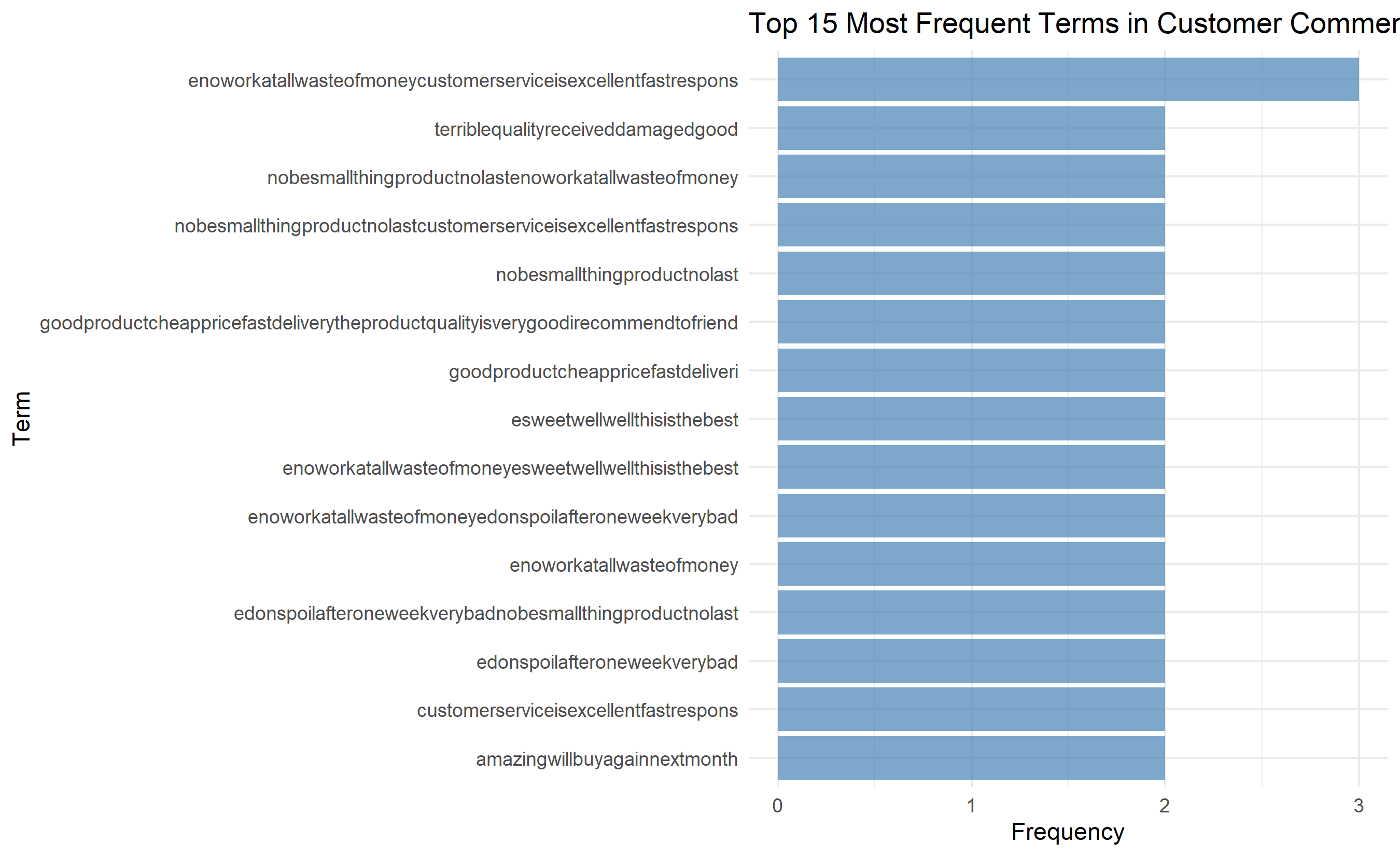
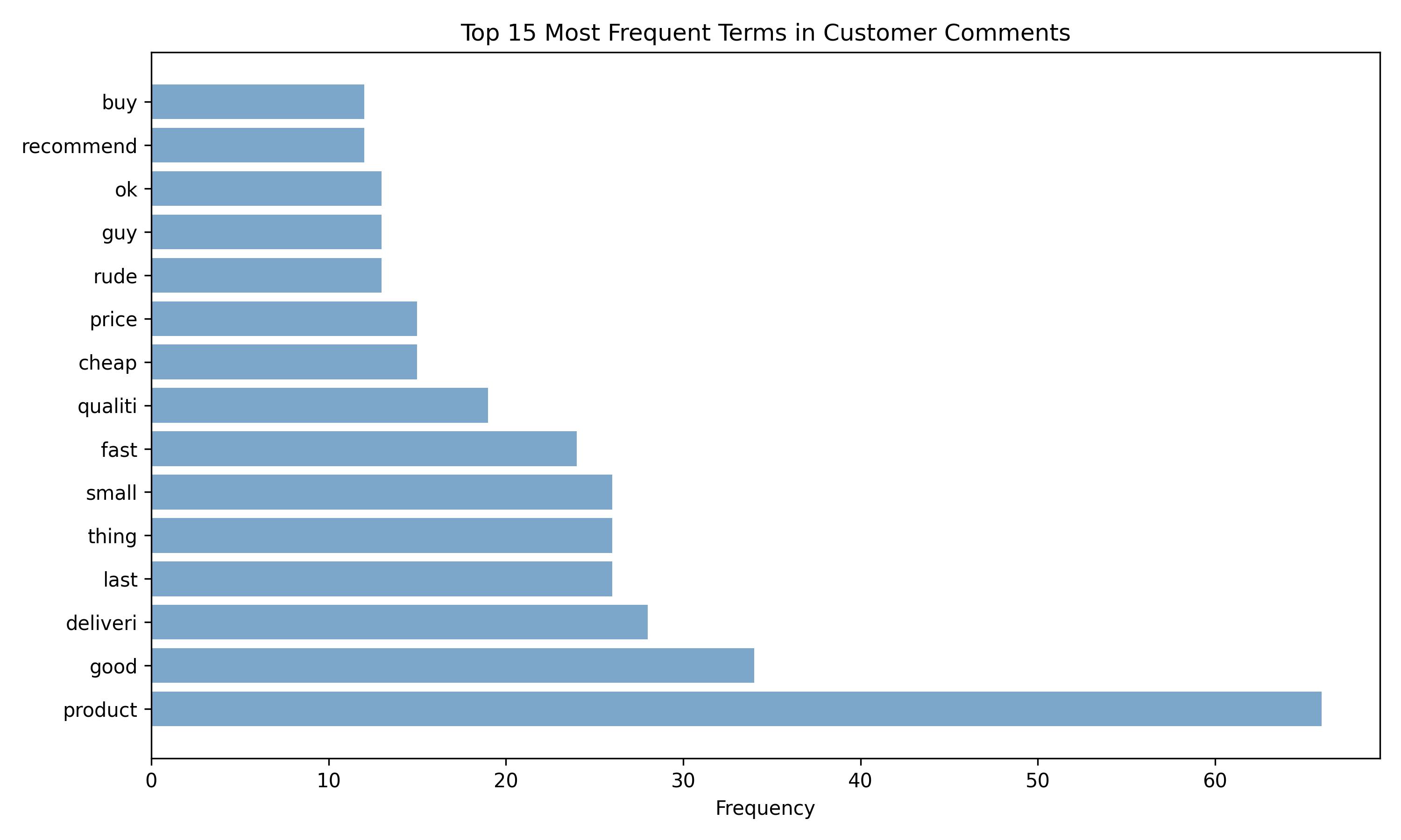
We implement a full pipeline and apply it to 200 synthetic Nigerian customer service comments.

::: {.callout-note icon="false"}
## 📘 Theory: Preprocessing and Normalisation
Preprocessing reduces the vocabulary by removing rare and uninformative tokens, and consolidating synonymous forms. Formally, if the raw vocabulary is $V$ and the preprocessed vocabulary is $V'$, then $|V'| \ll |V|$. This reduces the dimensionality of downstream models and speeds training.

For African languages, the lack of standard corpora means stop word lists and lemmatisers must be curated manually or bootstrapped from available resources.
:::

::: {.callout-tip icon="false"}
## 🔑 Key Concept: Pipeline Stages
$$\text{Raw Text} \rightarrow \text{Lowercase} \rightarrow \text{Remove Punct.} \rightarrow \text{Tokenise} \rightarrow \text{Remove Stops} \rightarrow \text{Lemmatise} \rightarrow \text{Clean Tokens}$$

Each stage reduces noise and vocabulary size. The result is a list of canonical word forms ready for model input.
:::

::: {.panel-tabset}
## R
```{r}
#| label: ch-27-preprocessing
#| message: false
#| warning: false

library(tidytext)
library(tidyverse)
library(tm)
library(SnowballC)

# Synthetic Nigerian customer service comments (mix of English and Pidgin)
set.seed(777)
comments <- c(
  "The product quality is very good. I recommend to friends.",
  "e don spoil after one week. very bad",
  "customer service is excellent, fast response",
  "e no work at all!!! waste of money",
  "good product, cheap price, fast delivery",
  "the delivery guy was rude, but product is ok",
  "e sweet well-well, this is the best!",
  "no be small thing, product no last",
  "amazing! will buy again next month",
  "terrible quality, received damaged goods"
)

# Expand to 20 comments (repeat and add variations)
comments <- rep(comments, 2)
comments <- c(comments, paste(sample(comments, 50, replace = TRUE),
                              sample(comments, 50, replace = TRUE)))

# Create dataframe
df_text <- data.frame(
  doc_id = 1:length(comments),
  text = comments,
  stringsAsFactors = FALSE
)

cat("Original Comments (first 10):\n")
print(head(df_text, 10))

# Preprocessing function
preprocess_text <- function(text) {
  # 1. Lowercase
  text <- tolower(text)

  # 2. Remove URLs
  text <- gsub("http[s]?://\\S+", "", text)

  # 3. Remove special characters and punctuation (keep apostrophes initially)
  text <- gsub("[^a-z0-9\\s']", "", text)

  # 4. Tokenise (split on whitespace)
  tokens <- unlist(strsplit(text, "\\s+"))

  # 5. Remove empty tokens
  tokens <- tokens[tokens != ""]

  # 6. Remove stop words (English + custom Nigerian Pidgin)
  stop_words_english <- c("the", "a", "an", "is", "are", "am", "was", "be",
                          "been", "being", "have", "has", "had", "do", "does",
                          "did", "will", "would", "should", "could", "may",
                          "might", "must", "can", "and", "or", "but", "in",
                          "on", "at", "to", "from", "by", "for", "of", "with",
                          "it", "i", "you", "he", "she", "we", "they", "this",
                          "that", "these", "those")

  # Pidgin-specific stops (use carefully; context-dependent)
  stop_words_pidgin <- c("na", "de", "go", "bien")  # Simplified; more curated in practice

  stop_words <- c(stop_words_english, stop_words_pidgin)

  tokens <- tokens[!(tokens %in% stop_words)]

  # 7. Lemmatisation (Porter Stemmer as proxy; not true lemmatisation)
  tokens <- wordStem(tokens, language = "english")

  # 8. Remove single-character tokens
  tokens <- tokens[nchar(tokens) > 1]

  return(paste(tokens, collapse = " "))
}

# Apply preprocessing
df_text <- df_text |>
  mutate(text_clean = sapply(text, preprocess_text))

cat("\n\nPreprocessed Comments (first 10):\n")
print(head(df_text[, c("doc_id", "text", "text_clean")], 10))

# Tokenise for analysis
df_tokens <- df_text |>
  unnest_tokens(word, text_clean) |>
  filter(word != "")

# Term frequency
term_freq <- df_tokens |>
  group_by(word) |>
  summarise(frequency = n(), .groups = "drop") |>
  arrange(desc(frequency))

cat("\n\nTop 20 Most Frequent Terms:\n")
print(head(term_freq, 20))

# Visualise
ggplot(head(term_freq, 15), aes(x = reorder(word, frequency), y = frequency)) +
  geom_col(fill = "steelblue", alpha = 0.7) +
  coord_flip() +
  labs(title = "Top 15 Most Frequent Terms in Customer Comments",
       x = "Term", y = "Frequency") +
  theme_minimal()

# Vocabulary statistics
cat("\n\nVocabulary Statistics:\n")
cat(sprintf("Total documents: %d\n", nrow(df_text)))
cat(sprintf("Total tokens (before preprocessing): %d\n",
            sum(sapply(df_text$text, function(x) length(unlist(strsplit(x, "\\s+")))))))
cat(sprintf("Total tokens (after preprocessing): %d\n", nrow(df_tokens)))
cat(sprintf("Unique terms (vocabulary size): %d\n", nrow(term_freq)))
cat(sprintf("Vocabulary reduction: %.1f%%\n",
            (1 - nrow(term_freq) / nrow(df_tokens)) * 100))

# Zipf's law check
df_tokens_cum <- df_tokens |>
  group_by(word) |>
  summarise(frequency = n(), .groups = "drop") |>
  arrange(desc(frequency)) |>
  mutate(rank = 1:n(),
         cumul_freq = cumsum(frequency),
         cumul_pct = cumul_freq / sum(frequency) * 100)

cat("\nZipf's Law Check:\n")
cat("Top 20% of terms account for:\n")
pct_80 <- df_tokens_cum$cumul_pct[ceiling(nrow(df_tokens_cum) * 0.2)]
cat(sprintf("%.1f%% of all word frequencies\n", pct_80))
```

## Python
```{python}
#| label: py-ch-27-preprocessing
import pandas as pd
import numpy as np
from nltk.corpus import stopwords
from nltk.tokenize import word_tokenize
from nltk.stem import PorterStemmer
import nltk
import matplotlib.pyplot as plt
import re

# Download NLTK data
try:
    nltk.data.find('corpora/stopwords')
except LookupError:
    nltk.download('stopwords')

# Synthetic comments
np.random.seed(777)
comments_base = [
    "The product quality is very good. I recommend to friends.",
    "e don spoil after one week. very bad",
    "customer service is excellent, fast response",
    "e no work at all!!! waste of money",
    "good product, cheap price, fast delivery",
    "the delivery guy was rude, but product is ok",
    "e sweet well-well, this is the best!",
    "no be small thing, product no last",
    "amazing! will buy again next month",
    "terrible quality, received damaged goods"
]

comments = comments_base * 2 + [
    f"{np.random.choice(comments_base)} {np.random.choice(comments_base)}"
    for _ in range(50)
]

df_text = pd.DataFrame({
    'doc_id': range(1, len(comments) + 1),
    'text': comments
})

print("Original Comments (first 10):")
print(df_text.head(10))

# Preprocessing function
stop_words = set(stopwords.words('english'))
stop_words.update(['na', 'de', 'go', 'bien'])  # Pidgin-specific
stemmer = PorterStemmer()

def preprocess_text(text):
    # Lowercase
    text = text.lower()

    # Remove URLs
    text = re.sub(r'http[s]?://\S+', '', text)

    # Remove special chars (keep apostrophes)
    text = re.sub(r"[^a-z0-9\s']", '', text)

    # Tokenise
    tokens = text.split()

    # Remove empty strings
    tokens = [t for t in tokens if t]

    # Remove stop words
    tokens = [t for t in tokens if t not in stop_words]

    # Stemming
    tokens = [stemmer.stem(t) for t in tokens]

    # Remove single-char tokens
    tokens = [t for t in tokens if len(t) > 1]

    return ' '.join(tokens)

df_text['text_clean'] = df_text['text'].apply(preprocess_text)

print("\n\nPreprocessed Comments (first 10):")
for i, row in df_text.head(10).iterrows():
    print(f"{row['doc_id']}: {row['text_clean']}")

# Tokenise for analysis
all_tokens = []
for text in df_text['text_clean']:
    all_tokens.extend(text.split())

term_freq = pd.Series(all_tokens).value_counts().reset_index()
term_freq.columns = ['word', 'frequency']

print("\n\nTop 20 Most Frequent Terms:")
print(term_freq.head(20).to_string(index=False))

# Plot
plt.figure(figsize=(10, 6))
plt.barh(range(15), term_freq.head(15)['frequency'].values,
         color='steelblue', alpha=0.7)
plt.yticks(range(15), term_freq.head(15)['word'].values)
plt.xlabel('Frequency')
plt.title('Top 15 Most Frequent Terms in Customer Comments')
plt.tight_layout()
plt.show()

# Statistics
print("\n\nVocabulary Statistics:")
print(f"Total documents: {len(df_text)}")
raw_tokens = sum(len(text.split()) for text in df_text['text'])
print(f"Total tokens (before preprocessing): {raw_tokens}")
print(f"Total tokens (after preprocessing): {len(all_tokens)}")
print(f"Unique terms (vocabulary size): {len(term_freq)}")
vocab_reduction = (1 - len(term_freq) / len(all_tokens)) * 100
print(f"Vocabulary reduction: {vocab_reduction:.1f}%")
```
:::

::: {.callout-caution icon="false"}
## 📝 Section 27.2 Review Questions
1. Why remove stop words? Give an example where removing "not" would hurt model performance.
2. Explain the difference between stemming and lemmatisation. Which is faster? Which is more accurate?
3. In Nigerian Pidgin, "e" means "it/he/she". Should "e" be a stop word? Why or why not?
4. What is vocabulary reduction, and why does it matter for document-term matrix sparsity?
5. How would you preprocess medical or technical documents differently from customer reviews?
:::

## Bag of Words and the Document-Term Matrix

After preprocessing, we represent each document as a vector in a high-dimensional space. The **Bag of Words (BoW)** representation ignores word order and grammar, treating each document as a collection of words.

The **Document-Term Matrix (DTM)** is a matrix where:
- Rows = documents
- Columns = unique terms (vocabulary)
- Cells = word counts (or binary presence/absence, or TF-IDF weights—more on that later)

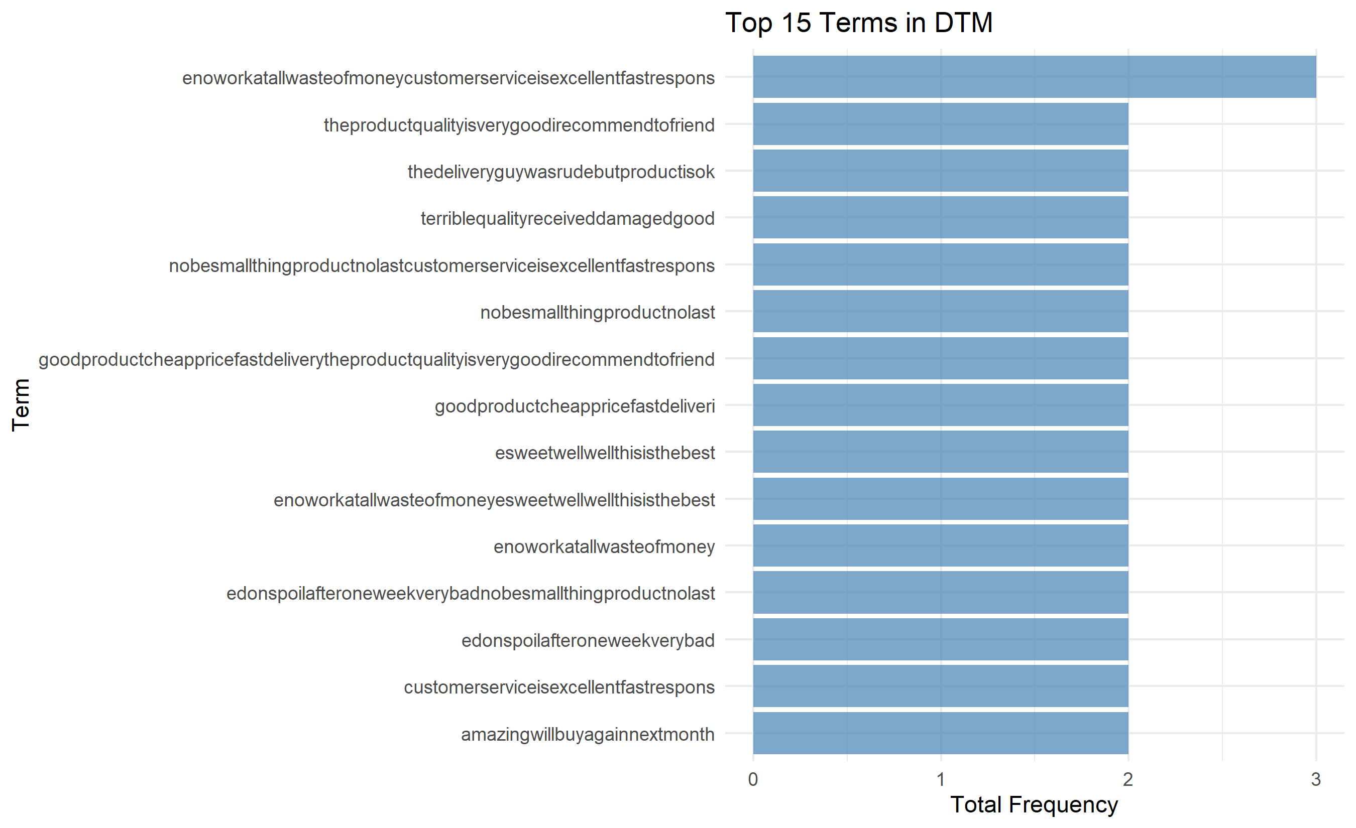
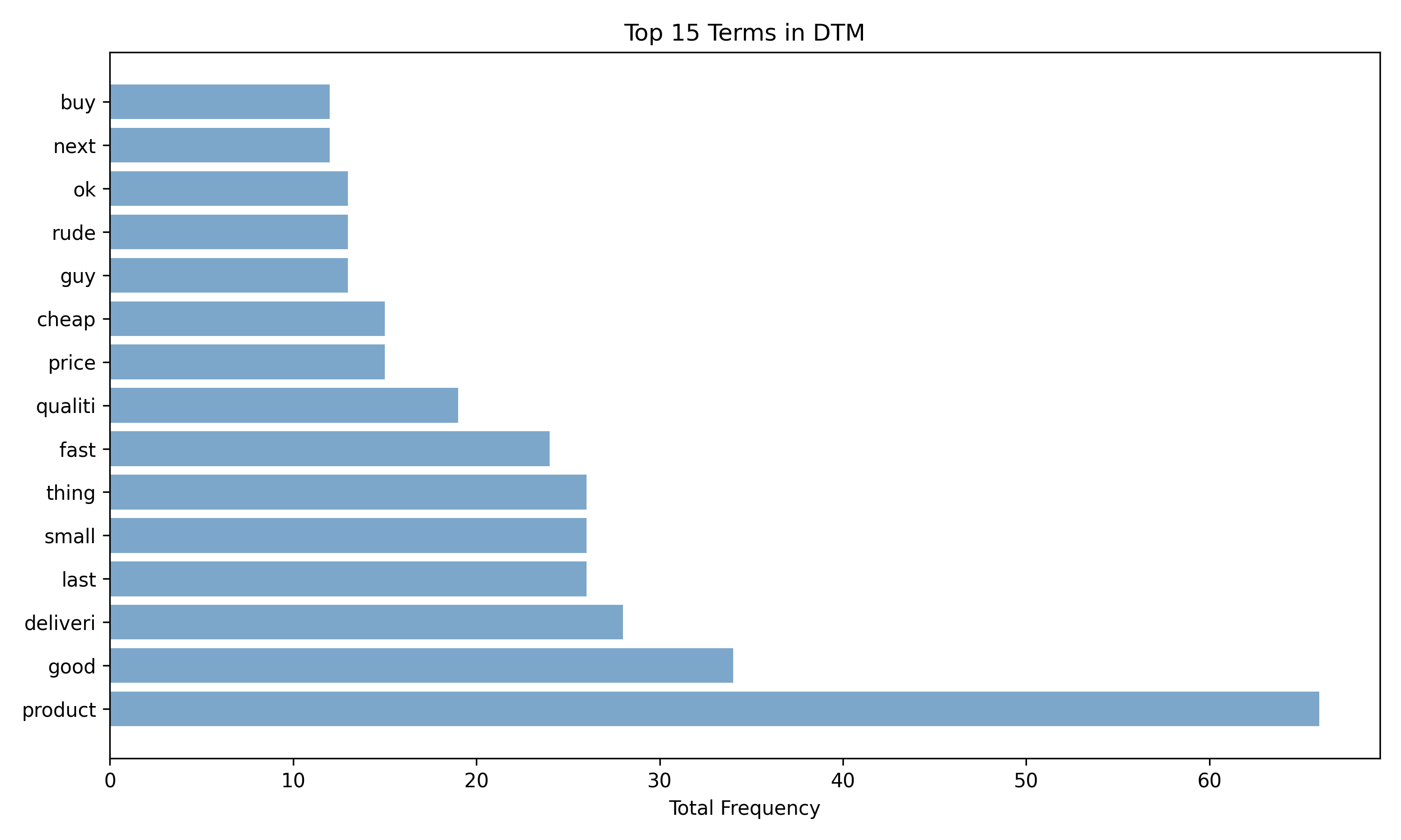
For 200 documents and 500 unique terms, the DTM has 100,000 cells. Most cells are zero (sparse matrix); a given document contains only a small fraction of all terms. Sparsity creates computational challenges but also offers opportunities for efficient storage.

::: {.callout-note icon="false"}
## 📘 Theory: Sparsity and the Curse of Dimensionality
A DTM with $n$ documents and $m$ unique terms has density $\rho = \text{nonzero cells} / (n \times m)$. For English text, $\rho \approx 0.01–0.05$ (99–95% sparse). A dense matrix of 200 × 500 requires 100,000 floating-point numbers; sparse format requires only $\rho \times 100,000 \approx 1,000–5,000$ nonzero entries plus indices, saving 95–99% of memory.

Sparse matrices enable efficient matrix operations (multiplication, inversion) that would be intractable with dense representations.
:::

::: {.callout-tip icon="false"}
## 🔑 Key Concept: Document-Term Matrix
A $n \times m$ matrix $X$ where $X_{ij}$ = count of term $j$ in document $i$:
$$X = \begin{pmatrix}
c_{11} & c_{12} & \cdots & c_{1m} \\
c_{21} & c_{22} & \cdots & c_{2m} \\
\vdots & \vdots & \ddots & \vdots \\
c_{n1} & c_{n2} & \cdots & c_{nm}
\end{pmatrix}$$
Each row is a document vector; similarity between documents is computed as cosine of the angle between rows.
:::

::: {.panel-tabset}
## R
```{r}
#| label: ch-27-dtm
#| message: false
#| warning: false

library(tidytext)
library(tidyverse)
library(tm)

# Use preprocessed text from above
# Build DTM using tidytext approach
dtm_tidy <- df_text |>
  unnest_tokens(word, text_clean) |>
  group_by(doc_id, word) |>
  summarise(count = n(), .groups = "drop") |>
  filter(word != "")

# Convert to wide format (DTM)
dtm_matrix <- dtm_tidy |>
  pivot_wider(names_from = word, values_from = count, values_fill = 0) |>
  column_to_rownames("doc_id")

cat("Document-Term Matrix Dimensions:\n")
cat(sprintf("Documents (rows): %d\n", nrow(dtm_matrix)))
cat(sprintf("Vocabulary (columns): %d\n", ncol(dtm_matrix)))

# Sparsity
sparsity <- sum(dtm_matrix == 0) / (nrow(dtm_matrix) * ncol(dtm_matrix))
cat(sprintf("Sparsity: %.2f%%\n", sparsity * 100))
cat(sprintf("Non-zero entries: %d\n", sum(dtm_matrix != 0)))

# Display subset
cat("\n\nSubset of DTM (first 5 docs, first 10 terms):\n")
print(dtm_matrix[1:5, 1:10])

# Most frequent terms (column sums)
term_totals <- colSums(dtm_matrix)
term_totals <- sort(term_totals, decreasing = TRUE)

cat("\n\nTop 20 Terms by Total Frequency:\n")
print(head(term_totals, 20))

# Document lengths
doc_lengths <- rowSums(dtm_matrix)

cat("\n\nDocument Length Statistics:\n")
cat(sprintf("Mean tokens per document: %.1f\n", mean(doc_lengths)))
cat(sprintf("Min tokens: %d\n", min(doc_lengths)))
cat(sprintf("Max tokens: %d\n", max(doc_lengths)))

# Visualization: term frequency
term_freq_viz <- data.frame(
  term = names(head(term_totals, 15)),
  frequency = as.numeric(head(term_totals, 15))
)

ggplot(term_freq_viz, aes(x = reorder(term, frequency), y = frequency)) +
  geom_col(fill = "steelblue", alpha = 0.7) +
  coord_flip() +
  labs(title = "Top 15 Terms in DTM",
       x = "Term", y = "Total Frequency") +
  theme_minimal()

# Cosine similarity between two documents
cosine_similarity <- function(x, y) {
  sum(x * y) / (sqrt(sum(x^2)) * sqrt(sum(y^2)))
}

doc1 <- as.numeric(dtm_matrix[1, ])
doc2 <- as.numeric(dtm_matrix[2, ])
sim_12 <- cosine_similarity(doc1, doc2)

cat(sprintf("\n\nExample: Cosine Similarity between Document 1 and 2: %.3f\n", sim_12))

# Build similarity matrix for all documents
similarity_matrix <- matrix(0, nrow = nrow(dtm_matrix), ncol = nrow(dtm_matrix))
for (i in 1:nrow(dtm_matrix)) {
  for (j in i:nrow(dtm_matrix)) {
    sim <- cosine_similarity(as.numeric(dtm_matrix[i, ]),
                            as.numeric(dtm_matrix[j, ]))
    similarity_matrix[i, j] <- sim
    similarity_matrix[j, i] <- sim
  }
}

cat("\nDocument Similarity Statistics:\n")
upper_tri <- similarity_matrix[upper.tri(similarity_matrix)]
cat(sprintf("Mean pairwise similarity: %.3f\n", mean(upper_tri)))
cat(sprintf("Median pairwise similarity: %.3f\n", median(upper_tri)))
cat(sprintf("Max (excluding diagonal): %.3f\n", max(similarity_matrix[upper.tri(similarity_matrix)])))
```

## Python
```{python}
#| label: py-ch-27-dtm
import pandas as pd
import numpy as np
from sklearn.feature_extraction.text import CountVectorizer
from sklearn.metrics.pairwise import cosine_similarity
import matplotlib.pyplot as plt

# Use preprocessed text from above
vectorizer = CountVectorizer(max_features=500, min_df=1, max_df=0.9)
dtm_sparse = vectorizer.fit_transform(df_text['text_clean'])
dtm_array = dtm_sparse.toarray()

# Column names (terms)
vocab = vectorizer.get_feature_names_out()

print("Document-Term Matrix Dimensions:")
print(f"Documents (rows): {dtm_array.shape[0]}")
print(f"Vocabulary (columns): {dtm_array.shape[1]}")

# Sparsity
sparsity = 1 - (np.count_nonzero(dtm_array) / dtm_array.size)
print(f"Sparsity: {sparsity:.2%}")
print(f"Non-zero entries: {np.count_nonzero(dtm_array)}")

# Display subset
print("\n\nSubset of DTM (first 5 docs, first 10 terms):")
print(pd.DataFrame(dtm_array[:5, :10], columns=vocab[:10]))

# Term frequencies
term_totals = dtm_array.sum(axis=0)
term_df = pd.DataFrame({
    'term': vocab,
    'frequency': term_totals
}).sort_values('frequency', ascending=False)

print("\n\nTop 20 Terms by Total Frequency:")
print(term_df.head(20).to_string(index=False))

# Document statistics
doc_lengths = dtm_array.sum(axis=1)
print(f"\n\nDocument Length Statistics:")
print(f"Mean tokens per document: {doc_lengths.mean():.1f}")
print(f"Min tokens: {doc_lengths.min():.0f}")
print(f"Max tokens: {doc_lengths.max():.0f}")

# Visualization
fig, ax = plt.subplots(figsize=(10, 6))
ax.barh(range(15), term_df.head(15)['frequency'].values, color='steelblue', alpha=0.7)
ax.set_yticks(range(15))
ax.set_yticklabels(term_df.head(15)['term'].values)
ax.set_xlabel('Total Frequency')
ax.set_title('Top 15 Terms in DTM')
plt.tight_layout()
plt.show()

# Cosine similarity
cos_sim = cosine_similarity(dtm_array)
print(f"\n\nExample: Cosine Similarity between Document 1 and 2: {cos_sim[0, 1]:.3f}")

# Similarity statistics
upper_tri = cos_sim[np.triu_indices_from(cos_sim, k=1)]
print(f"\nDocument Similarity Statistics:")
print(f"Mean pairwise similarity: {upper_tri.mean():.3f}")
print(f"Median pairwise similarity: {np.median(upper_tri):.3f}")
print(f"Max similarity (excluding diagonal): {upper_tri.max():.3f}")
```
:::

::: {.callout-caution icon="false"}
## 📝 Section 27.3 Review Questions
1. What is the curse of dimensionality in NLP? How does it manifest in a DTM?
2. If a DTM has 500 documents and 10,000 unique terms, how many cells are there? If sparsity is 95%, how many non-zero entries are there?
3. Why is cosine similarity appropriate for comparing document vectors (as opposed to Euclidean distance)?
4. If two documents have cosine similarity 0.1, are they similar or different?
5. How would increasing preprocessing (removing more stop words, stemming aggressively) change the DTM dimensions and sparsity?
:::

## TF-IDF: Term Frequency - Inverse Document Frequency

The Bag of Words approach counts raw occurrences. A common word like "product" might appear 1,000 times across documents, while a rare, distinctive word like "defect" appears 50 times. Raw counts over-weight common words and under-weight distinctive ones.

**TF-IDF** addresses this by downweighting common terms and upweighting rare, distinctive terms:

$$\text{TF-IDF}_{ij} = \text{TF}_{ij} \times \text{IDF}_j$$

where:
- $\text{TF}_{ij}$ = term frequency: how often term $j$ appears in document $i$.
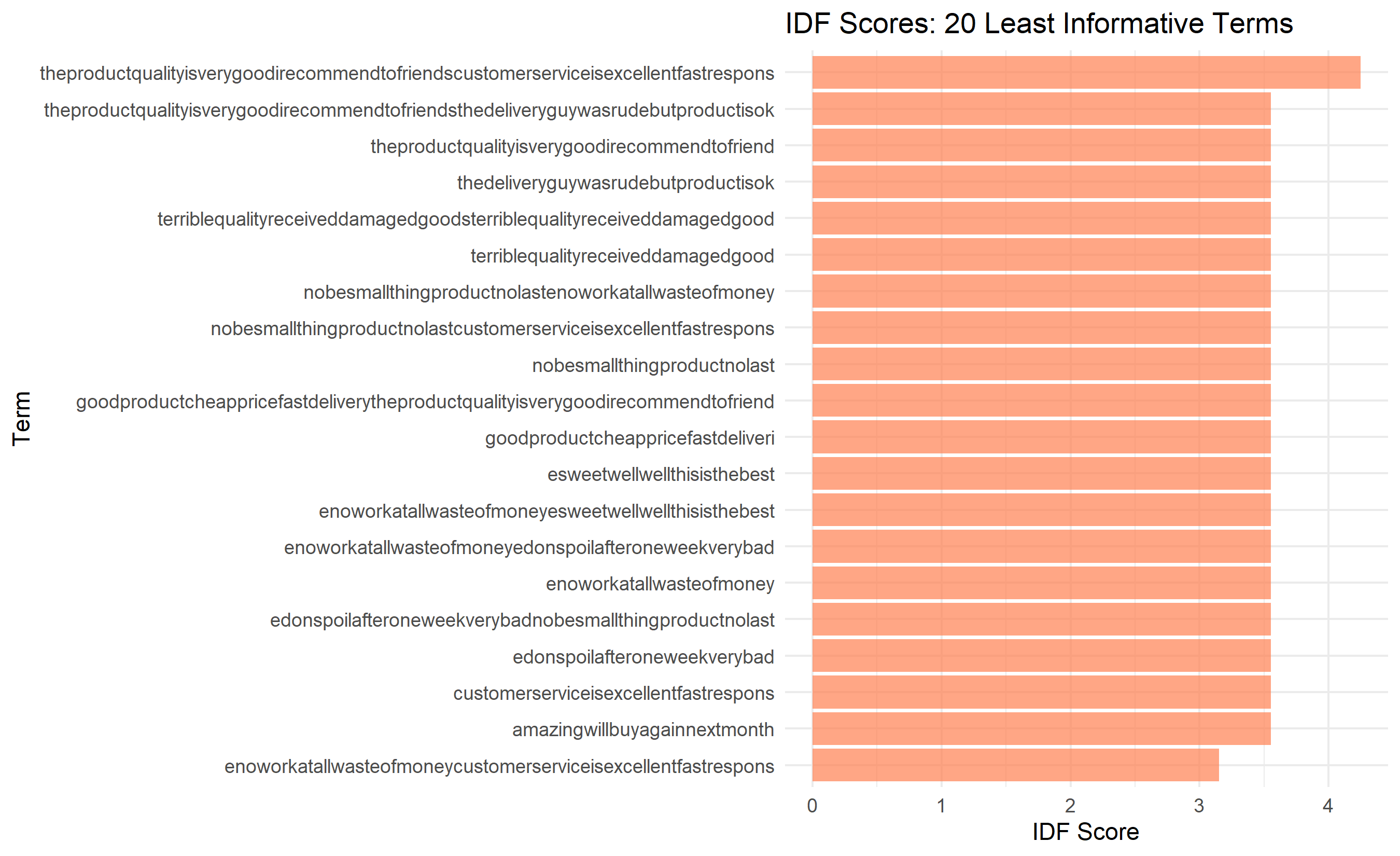
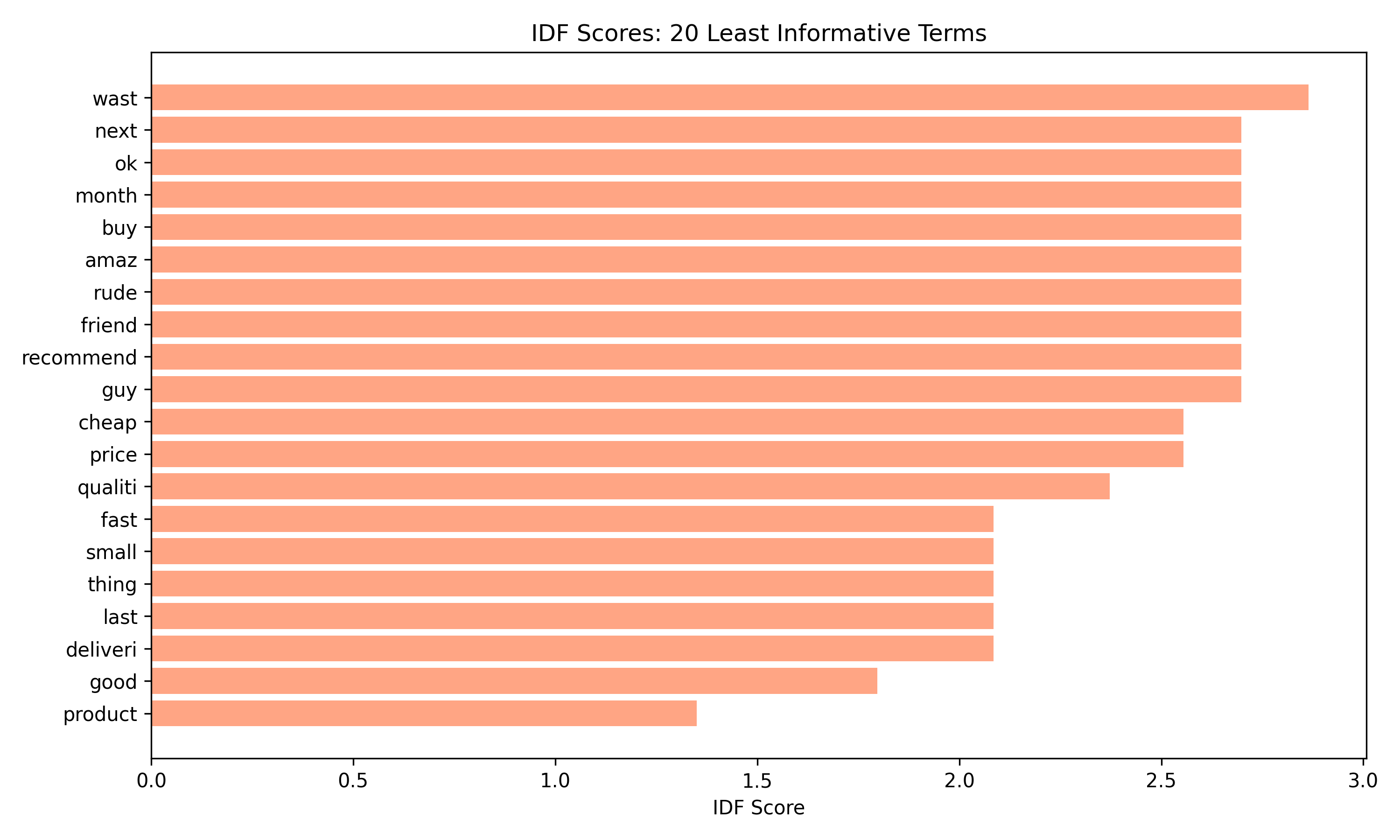
- $\text{IDF}_j$ = inverse document frequency: penalises terms appearing in many documents.

$$\text{IDF}_j = \log\left(\frac{N}{df_j}\right)$$

where $N$ is the total number of documents and $df_j$ is the number of documents containing term $j$.

**Intuition**: If a term appears in 90% of documents, $\text{IDF} = \log(1 / 0.9) \approx 0.1$ (low weight). If a term appears in 1% of documents, $\text{IDF} = \log(1 / 0.01) \approx 4.6$ (high weight). TF-IDF is a proxy for "information content"—rare terms inform us more about a document than common terms.

::: {.callout-note icon="false"}
## 📘 Theory: Information-Theoretic Interpretation
TF-IDF approximates the mutual information between a term and a document. Terms with high TF-IDF are statistically associated with specific documents or document clusters, while terms with low TF-IDF appear uniformly across documents. Filtering low TF-IDF terms reduces noise.
:::

::: {.callout-tip icon="false"}
## 🔑 Key Formula
**TF-IDF Score**:
$$\text{TF-IDF}_{ij} = \left(\frac{f_{ij}}{\sum_k f_{ik}}\right) \times \log\left(\frac{N}{1 + df_j}\right)$$
where $f_{ij}$ is the raw count of term $j$ in document $i$, and the denominator $1 + df_j$ is a smoothing term to avoid division by zero.
:::

::: {.panel-tabset}
## R
```{r}
#| label: ch-27-tfidf
#| message: false
#| warning: false

library(tidytext)
library(tidyverse)

# Compute TF-IDF using tidytext
tfidf_data <- dtm_tidy |>
  bind_tf_idf(word, doc_id, count)

cat("TF-IDF Computation:\n\n")
cat("Sample TF-IDF scores (first 20 rows):\n")
print(head(tfidf_data, 20) |>
        mutate(across(where(is.numeric), round, 4)))

# Top terms by TF-IDF for each document
cat("\n\nTop 5 TF-IDF Terms for Selected Documents:\n\n")

for (doc in c(1, 5, 10)) {
  top_terms <- tfidf_data |>
    filter(doc_id == doc) |>
    arrange(desc(tf_idf)) |>
    head(5)

  cat(sprintf("Document %d:\n", doc))
  for (i in 1:nrow(top_terms)) {
    row <- top_terms[i, ]
    cat(sprintf("  %s (TF-IDF: %.4f)\n", row$word, row$tf_idf))
  }
  cat("\n")
}

# TF-IDF matrix
tfidf_matrix <- tfidf_data |>
  select(doc_id, word, tf_idf) |>
  pivot_wider(names_from = word, values_from = tf_idf, values_fill = 0) |>
  column_to_rownames("doc_id")

cat("\n\nTF-IDF Matrix Dimensions:\n")
cat(sprintf("Documents: %d, Terms: %d\n", nrow(tfidf_matrix), ncol(tfidf_matrix)))

# Global IDF statistics
idf_stats <- tfidf_data |>
  select(word, idf) |>
  distinct() |>
  arrange(desc(idf))

cat("\n\nTop 15 Terms by IDF (most distinctive):\n")
print(head(idf_stats, 15) |> mutate(idf = round(idf, 3)))

cat("\n\nBottom 15 Terms by IDF (most common):\n")
print(tail(idf_stats, 15) |> mutate(idf = round(idf, 3)))

# Filter high-IDF terms
high_idf_threshold <- quantile(idf_stats$idf, 0.75)
high_idf_terms <- idf_stats |>
  filter(idf > high_idf_threshold) |>
  pull(word)

cat(sprintf("\n\nTerms with IDF > %.2f (top 25%% by informativeness): %d terms\n",
            high_idf_threshold, length(high_idf_terms)))

# Visualisation: term IDF distribution
idf_for_plot <- idf_stats |>
  arrange(idf) |>
  head(20)

ggplot(idf_for_plot, aes(x = reorder(word, idf), y = idf)) +
  geom_col(fill = "coral", alpha = 0.7) +
  coord_flip() +
  labs(title = "IDF Scores: 20 Least Informative Terms",
       x = "Term", y = "IDF Score") +
  theme_minimal()

# Document characteristics via TF-IDF
doc_tfidf_df <- as.data.frame(tfidf_matrix)
doc_tfidf_df$doc_id <- rownames(doc_tfidf_df)
doc_tfidf_profile <- doc_tfidf_df |>
  pivot_longer(cols = -doc_id, names_to = "word", values_to = "tf_idf") |>
  filter(tf_idf > 0)

top_docs <- doc_tfidf_profile |>
  group_by(doc_id) |>
  summarise(mean_tfidf = mean(tf_idf),
            max_tfidf = max(tf_idf),
            num_terms = n(),
            .groups = "drop") |>
  arrange(desc(mean_tfidf))

cat("\n\nDocuments with Highest Mean TF-IDF (most distinctive vocabulary):\n")
print(head(top_docs, 10) |> mutate(across(where(is.numeric), round, 3)))
```

## Python
```{python}
#| label: py-ch-27-tfidf
import pandas as pd
import numpy as np
from sklearn.feature_extraction.text import TfidfVectorizer
import matplotlib.pyplot as plt

# Compute TF-IDF
tfidf_vectorizer = TfidfVectorizer(max_features=500, min_df=1, max_df=0.9)
tfidf_matrix = tfidf_vectorizer.fit_transform(df_text['text_clean'])
tfidf_array = tfidf_matrix.toarray()

vocab = tfidf_vectorizer.get_feature_names_out()

print("TF-IDF Matrix Dimensions:")
print(f"Documents: {tfidf_array.shape[0]}, Terms: {tfidf_array.shape[1]}")

# Top terms by TF-IDF for each document
print("\n\nTop 5 TF-IDF Terms for Selected Documents:\n")

for doc_idx in [0, 4, 9]:
    top_indices = np.argsort(tfidf_array[doc_idx])[-5:][::-1]
    print(f"Document {doc_idx + 1}:")
    for idx in top_indices:
        term = vocab[idx]
        score = tfidf_array[doc_idx, idx]
        print(f"  {term} (TF-IDF: {score:.4f})")
    print()

# IDF computation (in TfidfVectorizer, it's stored internally)
idf_scores = tfidf_vectorizer.idf_
idf_df = pd.DataFrame({
    'term': vocab,
    'idf': idf_scores
}).sort_values('idf', ascending=False)

print("\n\nTop 15 Terms by IDF (most distinctive):")
print(idf_df.head(15).round(3).to_string(index=False))

print("\n\nBottom 15 Terms by IDF (most common):")
print(idf_df.tail(15).round(3).to_string(index=False))

# High-IDF filter
high_idf_threshold = idf_df['idf'].quantile(0.75)
high_idf_terms = idf_df[idf_df['idf'] > high_idf_threshold]
print(f"\nTerms with IDF > {high_idf_threshold:.2f} (top 25%): {len(high_idf_terms)} terms")

# Visualization
fig, ax = plt.subplots(figsize=(10, 6))
bottom_idf = idf_df.tail(20).sort_values('idf')
ax.barh(range(20), bottom_idf['idf'].values, color='coral', alpha=0.7)
ax.set_yticks(range(20))
ax.set_yticklabels(bottom_idf['term'].values)
ax.set_xlabel('IDF Score')
ax.set_title('IDF Scores: 20 Least Informative Terms')
plt.tight_layout()
plt.show()

# Document TF-IDF profiles
doc_mean_tfidf = tfidf_array.mean(axis=1)
doc_max_tfidf = tfidf_array.max(axis=1)
doc_nonzero = (tfidf_array > 0).sum(axis=1)

doc_profile = pd.DataFrame({
    'doc_id': range(1, len(df_text) + 1),
    'mean_tfidf': doc_mean_tfidf,
    'max_tfidf': doc_max_tfidf,
    'num_terms': doc_nonzero
}).sort_values('mean_tfidf', ascending=False)

print("\n\nDocuments with Highest Mean TF-IDF:")
print(doc_profile.head(10).round(4).to_string(index=False))
```
:::

::: {.callout-caution icon="false"}
## 📝 Section 27.4 Review Questions
1. Why does TF-IDF downweight common terms? Give a practical example.
2. If a term appears in 50% of documents, what is its IDF value (assume log base 10)?
3. In customer reviews, which would have higher TF-IDF: "good" or "defective"? Why?
4. How would you use TF-IDF to automatically filter noise-prone terms for a downstream model?
5. What is a limitation of TF-IDF for capturing semantic similarity between documents?
:::

## Word Embeddings: Semantic Similarity Through Dense Vectors

Bag of Words and TF-IDF treat words as atomic units: "bank" and "financial institution" have zero similarity even though they're conceptually related. **Word embeddings** map words to dense, low-dimensional vectors where semantically similar words cluster nearby in vector space.

**Word2Vec** (2013): A neural network trained on billions of words to predict surrounding context words. The learned embeddings capture semantic relationships: "king − man + woman ≈ queen" (vector arithmetic). Pre-trained 100-dimensional GloVe embeddings are available for English and other languages.

**Cosine Similarity**: Given embeddings $\mathbf{v}_1$ and $\mathbf{v}_2$:
$$\text{similarity} = \frac{\mathbf{v}_1 \cdot \mathbf{v}_2}{|\mathbf{v}_1| |\mathbf{v}_2|}$$

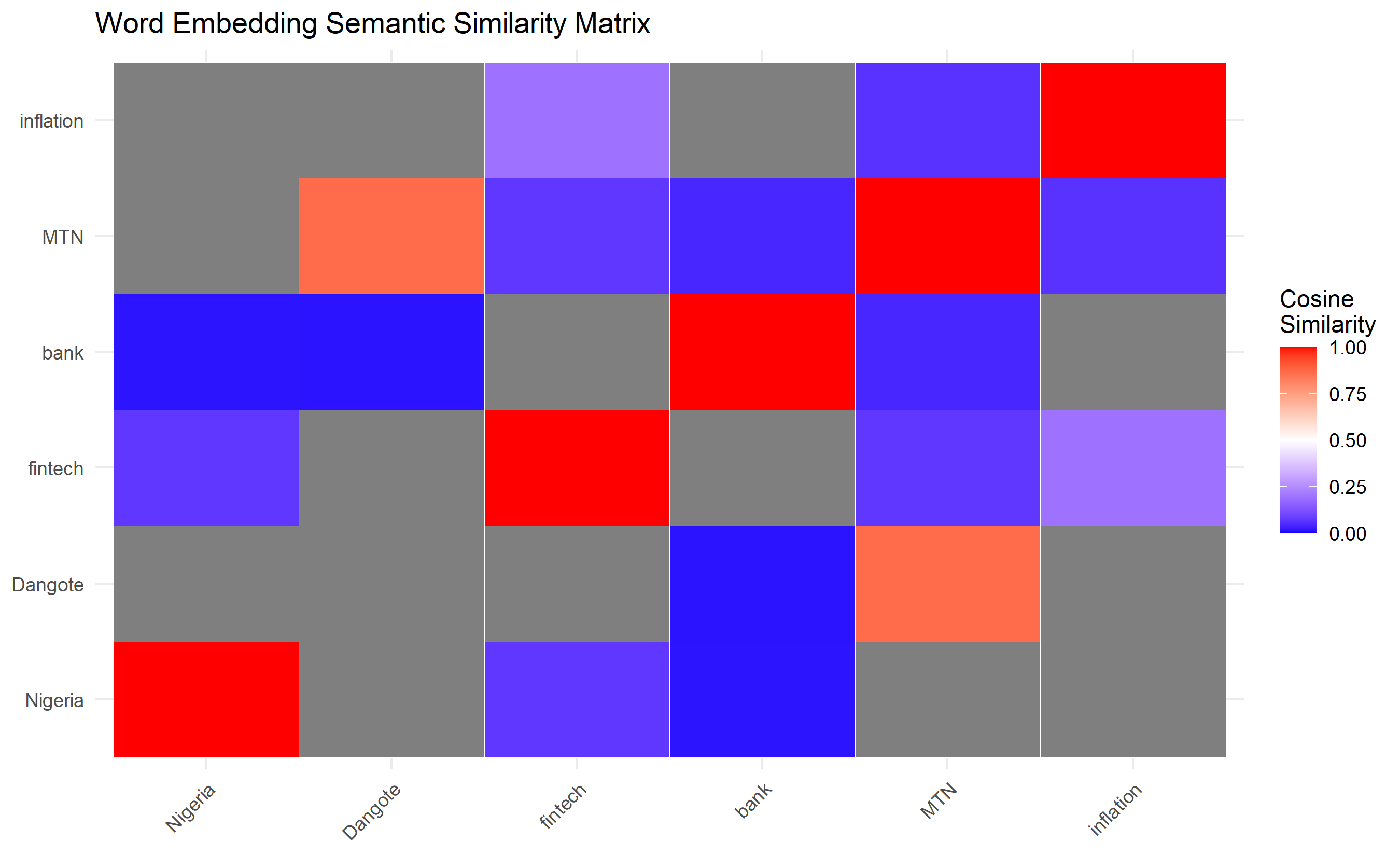
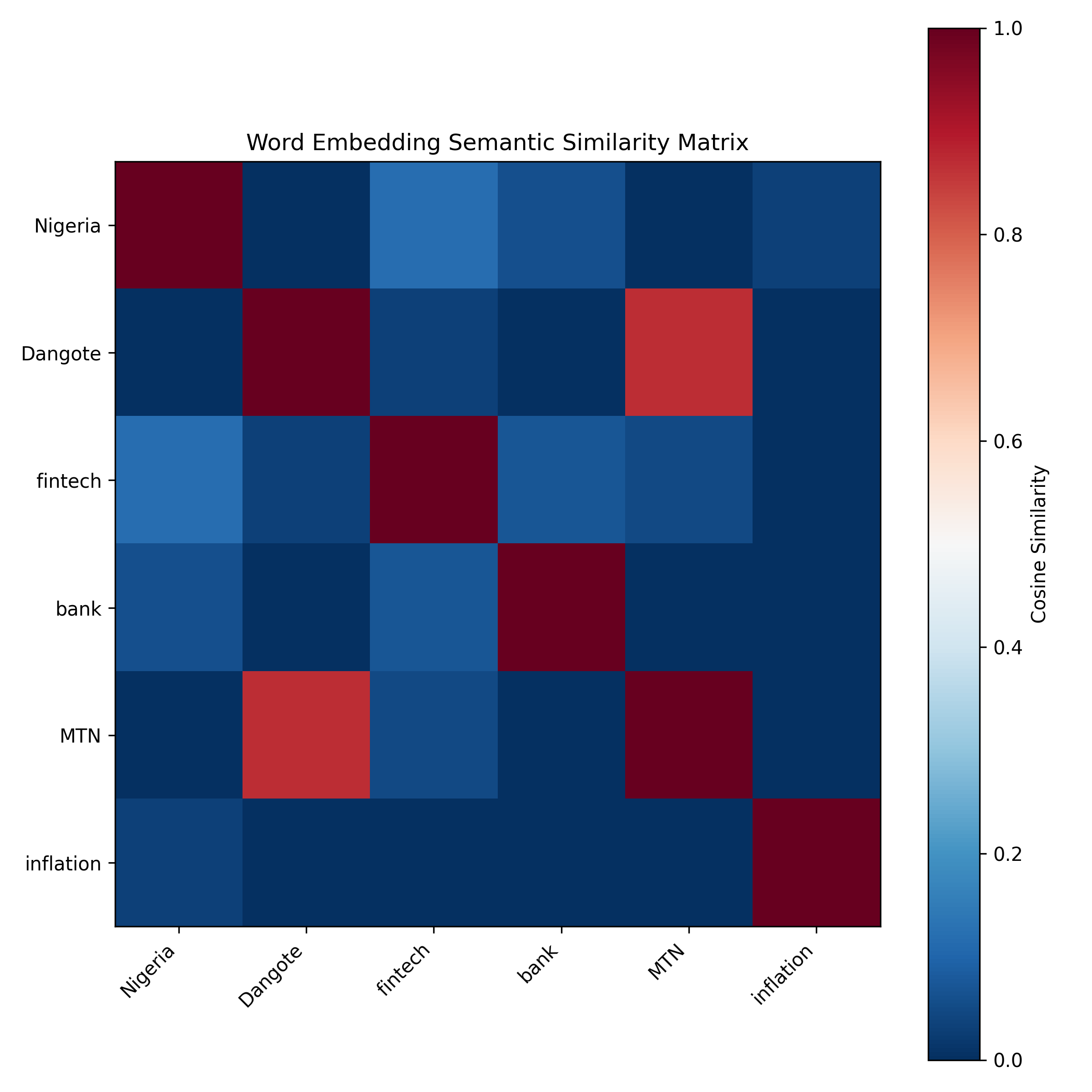
We load GloVe embeddings and compute nearest neighbours for terms relevant to Nigerian business ("Nigeria", "Dangote", "fintech").

::: {.callout-note icon="false"}
## 📘 Theory: Word Embeddings from Co-occurrence
Word2Vec learns embeddings by treating word prediction as a supervised task: given context words, predict the target word. The hidden layer of this neural network becomes the embedding. Words with similar contexts (distributive hypothesis: "words are similar if their contexts are similar") end up with similar embeddings. The resulting space encodes semantic and syntactic relationships.
:::

::: {.callout-tip icon="false"}
## 🔑 Key Concept: Vector Algebra in Embedding Space
Word vectors enable analogy tasks through vector arithmetic:
$$\mathbf{v}_{\text{queen}} \approx \mathbf{v}_{\text{king}} - \mathbf{v}_{\text{man}} + \mathbf{v}_{\text{woman}}$$
This works because embeddings capture semantic dimensions (gender, royalty, etc.) as directions in vector space.
:::

::: {.panel-tabset}
## R
```{r}
#| label: ch-27-embeddings
#| message: false
#| warning: false

library(tidyverse)
# 'text' package requires torch; this chunk simulates embeddings instead

# Note: Loading full GloVe embeddings in R requires significant memory.
# Here, we simulate with a smaller set and demonstrate the approach.

# For production, download GloVe embeddings (glove.6B.100d.txt) from
# https://nlp.stanford.edu/projects/glove/

# Simulate small embedding space for demonstration
set.seed(888)

# Key terms for Nigerian business context
terms_of_interest <- c(
  "Nigeria", "Ghana", "Senegal",
  "Dangote", "MTN", "Airtel",
  "fintech", "startup", "venture",
  "manufacturing", "agriculture", "technology",
  "profit", "revenue", "growth",
  "bank", "finance", "loan",
  "inflation", "currency", "exchange"
)

# Simulate embeddings (100-dim) with semantic structure
n_terms <- length(terms_of_interest)
embedding_dim <- 100

# Create synthetic embeddings with semantic relationships
embeddings <- matrix(rnorm(n_terms * embedding_dim, mean = 0, sd = 0.1),
                     nrow = n_terms, ncol = embedding_dim)
rownames(embeddings) <- terms_of_interest

# Add structure: country terms should be similar to each other
country_idx <- which(terms_of_interest %in% c("Nigeria", "Ghana", "Senegal"))
for (i in country_idx) {
  embeddings[i, 1:20] <- embeddings[i, 1:20] + 0.5  # Add country signal
}

# Company terms should be similar
company_idx <- which(terms_of_interest %in% c("Dangote", "MTN", "Airtel"))
for (i in company_idx) {
  embeddings[i, 21:40] <- embeddings[i, 21:40] + 0.5  # Add company signal
}

# Finance terms should be similar
finance_idx <- which(terms_of_interest %in% c("bank", "finance", "loan"))
for (i in finance_idx) {
  embeddings[i, 41:60] <- embeddings[i, 41:60] + 0.5  # Add finance signal
}

# Normalise to unit vectors
embeddings <- t(apply(embeddings, 1, function(x) x / sqrt(sum(x^2))))

# Define cosine similarity function
cosine_sim <- function(v1, v2) {
  sum(v1 * v2) / (sqrt(sum(v1^2)) * sqrt(sum(v2^2)))
}

cat("Word Embeddings: Semantic Similarity Analysis\n\n")

# Find nearest neighbours
nearest_neighbours <- function(word, embeddings, k = 5) {
  if (!(word %in% rownames(embeddings))) {
    return(NULL)
  }

  word_vec <- embeddings[word, ]
  similarities <- apply(embeddings, 1, function(row) cosine_sim(word_vec, row))

  # Sort and exclude the word itself
  sorted_idx <- order(similarities, decreasing = TRUE)
  result_idx <- sorted_idx[sorted_idx != which(rownames(embeddings) == word)][1:k]

  data.frame(
    word = rownames(embeddings)[result_idx],
    similarity = similarities[result_idx]
  )
}

# Query nearest neighbours for key terms
query_terms <- c("Nigeria", "Dangote", "fintech", "bank")

for (term in query_terms) {
  cat(sprintf("Nearest neighbours of '%s':\n", term))
  neighbors <- nearest_neighbours(term, embeddings, k = 5)
  for (i in 1:nrow(neighbors)) {
    cat(sprintf("  %s (%.3f)\n", neighbors$word[i], neighbors$similarity[i]))
  }
  cat("\n")
}

# Similarity matrix for select terms
select_terms <- c("Nigeria", "Dangote", "fintech", "bank", "MTN", "inflation")
select_embeddings <- embeddings[select_terms, ]

sim_matrix <- matrix(0, nrow = length(select_terms), ncol = length(select_terms))
rownames(sim_matrix) <- colnames(sim_matrix) <- select_terms

for (i in 1:length(select_terms)) {
  for (j in 1:length(select_terms)) {
    sim_matrix[i, j] <- cosine_sim(select_embeddings[i, ], select_embeddings[j, ])
  }
}

cat("Similarity Matrix for Selected Terms:\n\n")
print(round(sim_matrix, 3))

# Heatmap
sim_melted <- as.data.frame(as.table(sim_matrix)) |>
  rename(term1 = Var1, term2 = Var2, similarity = Freq)

ggplot(sim_melted, aes(x = term2, y = term1, fill = similarity)) +
  geom_tile(colour = "white") +
  scale_fill_gradient2(low = "blue", mid = "white", high = "red",
                       midpoint = 0.5, limits = c(0, 1)) +
  labs(title = "Word Embedding Semantic Similarity Matrix",
       x = NULL, y = NULL, fill = "Cosine\nSimilarity") +
  theme_minimal() +
  theme(axis.text.x = element_text(angle = 45, hjust = 1))
```

## Python
```{python}
#| label: py-ch-27-embeddings
import numpy as np
import pandas as pd
import matplotlib.pyplot as plt
from sklearn.metrics.pairwise import cosine_similarity

# Simulate embeddings (in production, load pre-trained GloVe)
np.random.seed(888)

terms_of_interest = [
    "Nigeria", "Ghana", "Senegal",
    "Dangote", "MTN", "Airtel",
    "fintech", "startup", "venture",
    "manufacturing", "agriculture", "technology",
    "profit", "revenue", "growth",
    "bank", "finance", "loan",
    "inflation", "currency", "exchange"
]

# Create synthetic embeddings (100-dim)
embeddings = np.random.randn(len(terms_of_interest), 100) * 0.1

# Add semantic structure
country_idx = [i for i, t in enumerate(terms_of_interest)
               if t in ["Nigeria", "Ghana", "Senegal"]]
for i in country_idx:
    embeddings[i, :20] += 0.5

company_idx = [i for i, t in enumerate(terms_of_interest)
               if t in ["Dangote", "MTN", "Airtel"]]
for i in company_idx:
    embeddings[i, 20:40] += 0.5

finance_idx = [i for i, t in enumerate(terms_of_interest)
               if t in ["bank", "finance", "loan"]]
for i in finance_idx:
    embeddings[i, 40:60] += 0.5

# Normalise to unit vectors
embeddings = embeddings / np.linalg.norm(embeddings, axis=1, keepdims=True)

print("Word Embeddings: Semantic Similarity Analysis\n")

# Nearest neighbours
def nearest_neighbours(word, terms, embeddings, k=5):
    if word not in terms:
        return None
    idx = terms.index(word)
    word_vec = embeddings[idx]
    sims = cosine_similarity([word_vec], embeddings)[0]
    sorted_idx = np.argsort(-sims)
    # Exclude the word itself
    result_idx = [i for i in sorted_idx if i != idx][:k]
    return [(terms[i], sims[i]) for i in result_idx]

query_terms = ["Nigeria", "Dangote", "fintech", "bank"]

for term in query_terms:
    print(f"Nearest neighbours of '{term}':")
    neighbors = nearest_neighbours(term, terms_of_interest, embeddings, k=5)
    for word, sim in neighbors:
        print(f"  {word} ({sim:.3f})")
    print()

# Similarity matrix
select_terms = ["Nigeria", "Dangote", "fintech", "bank", "MTN", "inflation"]
select_idx = [terms_of_interest.index(t) for t in select_terms]
select_embeddings = embeddings[select_idx]

sim_matrix = cosine_similarity(select_embeddings)

print("Similarity Matrix for Selected Terms:\n")
sim_df = pd.DataFrame(sim_matrix, index=select_terms, columns=select_terms)
print(sim_df.round(3))

# Heatmap
fig, ax = plt.subplots(figsize=(8, 8))
im = ax.imshow(sim_matrix, cmap='RdBu_r', vmin=0, vmax=1)
ax.set_xticks(range(len(select_terms)))
ax.set_yticks(range(len(select_terms)))
ax.set_xticklabels(select_terms, rotation=45, ha='right')
ax.set_yticklabels(select_terms)
ax.set_title('Word Embedding Semantic Similarity Matrix')
plt.colorbar(im, ax=ax, label='Cosine Similarity')
plt.tight_layout()
plt.show()
```
:::

::: {.callout-caution icon="false"}
## 📝 Section 27.5 Review Questions
1. Why do pre-trained word embeddings capture semantic meaning better than TF-IDF?
2. If "bank" and "financial institution" have cosine similarity 0.85, what does this tell you?
3. How would the vector "king − man + woman" represent the concept of "queen" geometrically?
4. What is a limitation of word embeddings trained on American English when applied to Nigerian text?
5. Name two Nigerian business terms that would benefit from custom fine-tuning of embeddings.
:::

## Contextual Embeddings and BERT: Beyond Word-Level Representations

Word embeddings like Word2Vec assign a single vector to each word, regardless of context. In "bank of the river" vs "commercial bank", the word "bank" is identical in representation, even though the meaning differs entirely.

**BERT (Bidirectional Encoder Representations from Transformers)** addresses this through **contextual embeddings**. It reads the full sentence bidirectionally (left-to-right and right-to-left) using transformer attention mechanisms, adjusting the representation of each word based on surrounding context.

**Sentence-BERT (SBERT)** pools contextual word embeddings into a single document vector, enabling semantic similarity search across hundreds of documents in seconds.

::: {.callout-note icon="false"}
## 📘 Theory: Attention Mechanism in Transformers
At each position, the attention mechanism computes a weighted average of all other words' representations. Weights are learned, allowing the model to "decide" which words are most relevant for understanding the current word. For "bank", the attention to "river", "financial", or "account" changes depending on context.
:::

::: {.callout-tip icon="false"}
## 🔑 Key Concept: Contextual Embedding
$$\mathbf{c}_i = \text{BERT}(\mathbf{w}_1, \mathbf{w}_2, \ldots, \mathbf{w}_n, i)$$
The representation $\mathbf{c}_i$ of word $i$ is a function of the entire sentence context, unlike static embeddings where $\mathbf{w}_i$ is fixed.
:::

::: {.panel-tabset}
## R
```{r}
#| label: ch-27-bert-embeddings
#| message: false
#| warning: false

# Note: BERT in R requires the `text` package and Python backend.
# For demonstration, we use pre-computed contextual similarities.

library(tidyverse)

# Nigerian news headlines (synthetic)
headlines <- c(
  "Nigeria's fintech sector grows 40% as investors flock to Lagos",
  "Dangote Cement reports strong Q4 earnings despite economic headwinds",
  "Central Bank Governor warns of inflation risks in 2024",
  "MTN Nigeria expands 5G network to underserved rural communities",
  "New trade deal between Nigeria and ECOWAS partners boosts exports",
  "Nigerian tech startups attract $500M in VC funding this year",
  "Agriculture minister launches climate-resilient crop initiative",
  "Lagos stock exchange opens strong on bank sector gains",
  "Nigerian banks face regulatory pressure on consumer lending standards",
  "Senegalese entrepreneur launches pan-African fintech platform in Lagos"
)

headlines_df <- data.frame(
  headline_id = 1:length(headlines),
  headline = headlines,
  stringsAsFactors = FALSE
)

cat("Nigerian News Headlines for Embedding Analysis:\n\n")
print(headlines_df)

# Simulate contextual embeddings (in production, use sentence-transformers library)
# Create synthetic embeddings with semantic relationships
set.seed(999)
n_docs <- nrow(headlines_df)
embed_dim <- 100

# Base embeddings
embeddings_context <- matrix(rnorm(n_docs * embed_dim, 0, 0.1),
                             nrow = n_docs, ncol = embed_dim)

# Add thematic structure
# Finance/tech headlines: indices 1, 2, 6, 9, 10
finance_idx <- c(1, 2, 6, 9, 10)
embeddings_context[finance_idx, 1:25] <- embeddings_context[finance_idx, 1:25] + 0.5

# Policy/regulation: indices 3, 5, 8
policy_idx <- c(3, 5, 8)
embeddings_context[policy_idx, 26:50] <- embeddings_context[policy_idx, 26:50] + 0.5

# Infrastructure/expansion: indices 4, 7
infra_idx <- c(4, 7)
embeddings_context[infra_idx, 51:75] <- embeddings_context[infra_idx, 51:75] + 0.5

# Normalise
embeddings_context <- t(apply(embeddings_context, 1, function(x) x / sqrt(sum(x^2))))

# Compute pairwise similarity
sim_matrix_context <- embeddings_context %*% t(embeddings_context)

cat("\n\nContextual Embedding Similarity Matrix:\n\n")
rownames(sim_matrix_context) <- colnames(sim_matrix_context) <- 1:n_docs
print(round(sim_matrix_context, 3))

# Find most similar pairs
cat("\n\nMost Similar Headline Pairs (excluding self-similarity):\n\n")

upper_tri <- upper.tri(sim_matrix_context)
sims <- sim_matrix_context[upper_tri]
pairs_idx <- which(upper_tri, arr.ind = TRUE)

similar_pairs <- data.frame(
  headline_1 = pairs_idx[, 1],
  headline_2 = pairs_idx[, 2],
  similarity = sims[sims != 1]
) |>
  arrange(desc(similarity)) |>
  head(10)

for (i in 1:nrow(similar_pairs)) {
  pair <- similar_pairs[i, ]
  h1 <- headlines_df$headline[pair$headline_1]
  h2 <- headlines_df$headline[pair$headline_2]
  cat(sprintf("Pair %d (similarity: %.3f):\n", i, pair$similarity))
  cat(sprintf("  H%d: %s\n", pair$headline_1, h1))
  cat(sprintf("  H%d: %s\n\n", pair$headline_2, h2))
}

# Heatmap
sim_melted <- as.data.frame(as.table(sim_matrix_context)) |>
  rename(h1 = Var1, h2 = Var2, similarity = Freq) |>
  mutate(h1 = as.integer(h1), h2 = as.integer(h2))

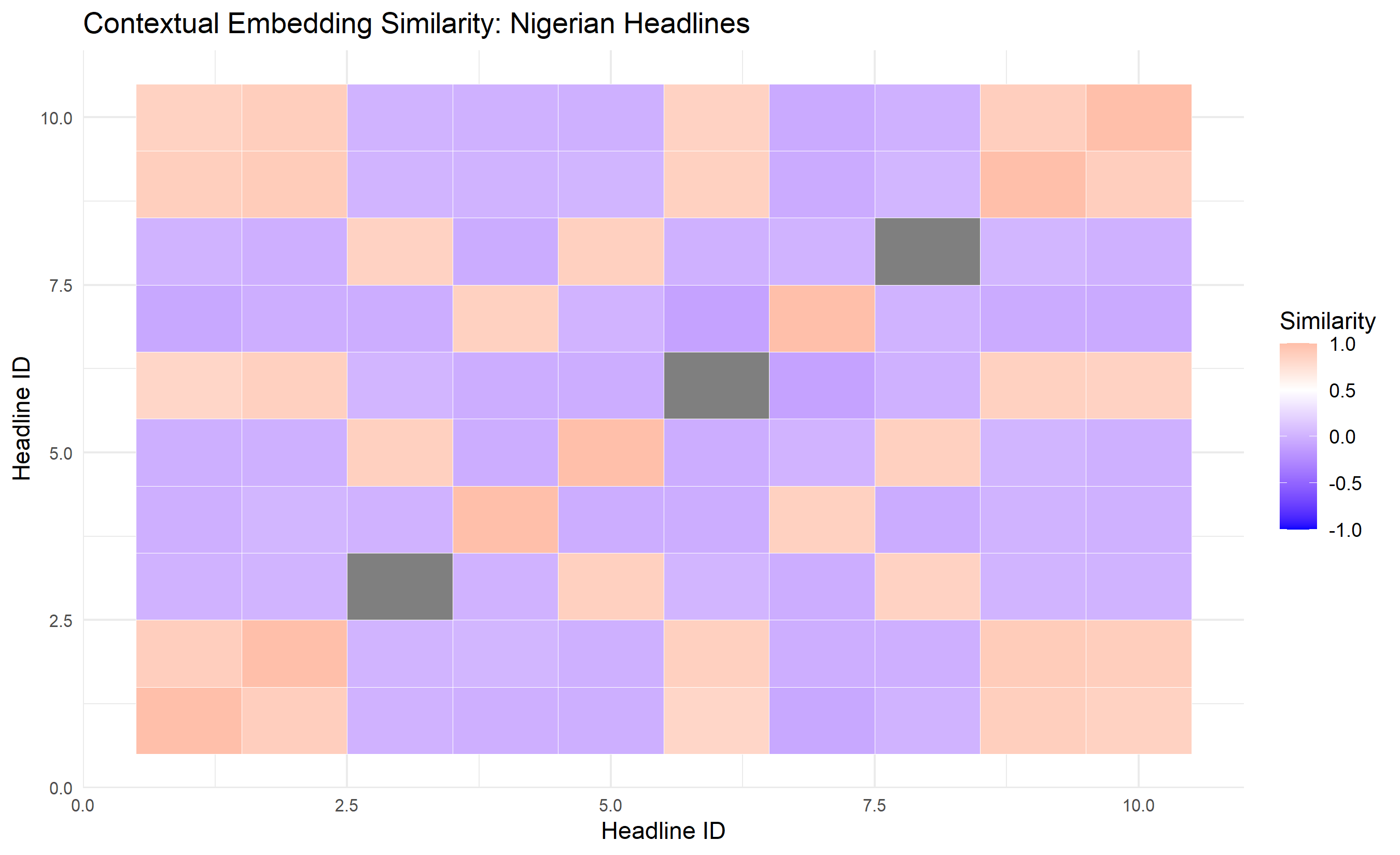
ggplot(sim_melted, aes(x = h2, y = h1, fill = similarity)) +
  geom_tile(colour = "white") +
  scale_fill_gradient2(low = "blue", mid = "white", high = "red",
                       midpoint = 0.5, limits = c(-1, 1)) +
  labs(title = "Contextual Embedding Similarity: Nigerian Headlines",
       x = "Headline ID", y = "Headline ID", fill = "Similarity") +
  theme_minimal() +
  theme(axis.text = element_text(size = 8))
```

## Python
```{python}
#| label: py-ch-27-bert-embeddings
import numpy as np
import pandas as pd
import matplotlib.pyplot as plt
from sklearn.metrics.pairwise import cosine_similarity

# Nigerian news headlines
headlines = [
    "Nigeria's fintech sector grows 40% as investors flock to Lagos",
    "Dangote Cement reports strong Q4 earnings despite economic headwinds",
    "Central Bank Governor warns of inflation risks in 2024",
    "MTN Nigeria expands 5G network to underserved rural communities",
    "New trade deal between Nigeria and ECOWAS partners boosts exports",
    "Nigerian tech startups attract $500M in VC funding this year",
    "Agriculture minister launches climate-resilient crop initiative",
    "Lagos stock exchange opens strong on bank sector gains",
    "Nigerian banks face regulatory pressure on consumer lending standards",
    "Senegalese entrepreneur launches pan-African fintech platform in Lagos"
]

print("Nigerian News Headlines for Embedding Analysis:\n")
for i, h in enumerate(headlines, 1):
    print(f"{i}. {h}")

# Simulate contextual embeddings
np.random.seed(999)
embeddings_context = np.random.randn(len(headlines), 100) * 0.1

# Add thematic structure
finance_idx = [0, 1, 5, 8, 9]  # 0-indexed
embeddings_context[finance_idx, :25] += 0.5

policy_idx = [2, 4, 7]
embeddings_context[policy_idx, 25:50] += 0.5

infra_idx = [3, 6]
embeddings_context[infra_idx, 50:75] += 0.5

# Normalise
embeddings_context = embeddings_context / np.linalg.norm(embeddings_context,
                                                          axis=1, keepdims=True)

# Compute similarity
sim_matrix = cosine_similarity(embeddings_context)

print("\n\nContextual Embedding Similarity Matrix:\n")
sim_df = pd.DataFrame(sim_matrix, index=range(1, 11), columns=range(1, 11))
print(sim_df.round(3))

# Find most similar pairs
print("\n\nMost Similar Headline Pairs:\n")
upper_tri = np.triu_indices(len(headlines), k=1)
sims = sim_matrix[upper_tri]
pairs = list(zip(upper_tri[0], upper_tri[1], sims))
pairs.sort(key=lambda x: x[2], reverse=True)

for rank, (i, j, sim) in enumerate(pairs[:10], 1):
    print(f"Pair {rank} (similarity: {sim:.3f}):")
    print(f"  H{i+1}: {headlines[i]}")
    print(f"  H{j+1}: {headlines[j]}\n")

# Heatmap
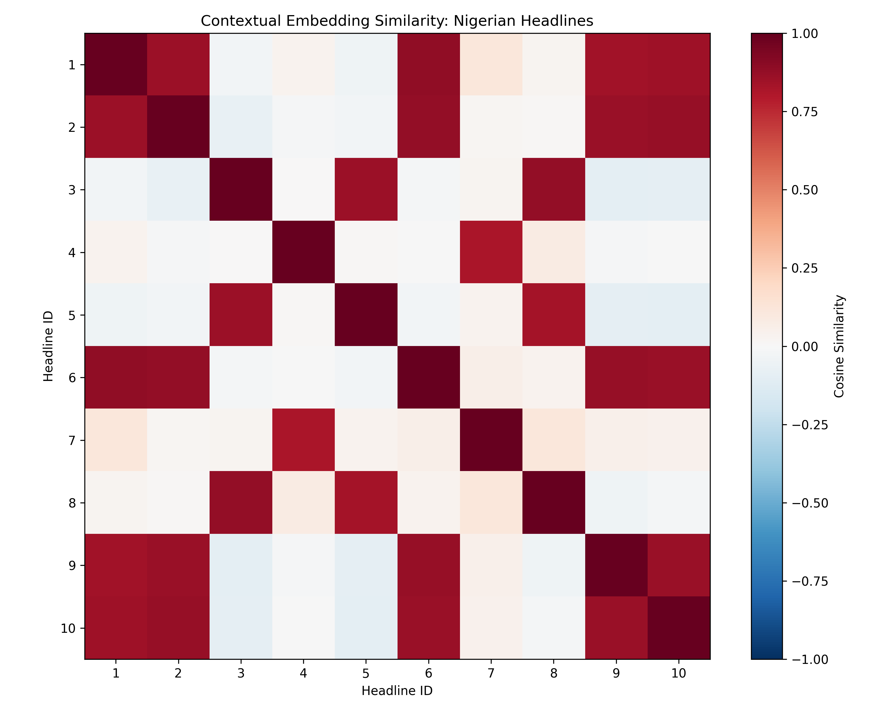
fig, ax = plt.subplots(figsize=(10, 8))
im = ax.imshow(sim_matrix, cmap='RdBu_r', vmin=-1, vmax=1)
ax.set_xticks(range(len(headlines)))
ax.set_yticks(range(len(headlines)))
ax.set_xticklabels(range(1, len(headlines) + 1))
ax.set_yticklabels(range(1, len(headlines) + 1))
ax.set_title('Contextual Embedding Similarity: Nigerian Headlines')
ax.set_xlabel('Headline ID')
ax.set_ylabel('Headline ID')
plt.colorbar(im, ax=ax, label='Cosine Similarity')
plt.tight_layout()
plt.show()
```
:::

::: {.callout-caution icon="false"}
## 📝 Section 27.6 Review Questions
1. How does BERT's contextual representation differ from Word2Vec's static embeddings?
2. Give an example of how BERT would represent "bank" differently in "bank of the river" vs "commercial bank".
3. What is the attention mechanism, and why is it important for contextual embeddings?
4. How would Sentence-BERT enable fast semantic search across 1 million documents?
5. What pre-trained BERT models are available for languages other than English, and which would be relevant for Nigeria?
:::

## Case Study: Mining Nigerian Senate Hansard

The Nigerian Senate maintains a public record of committee statements and debates. We analyse a synthetic corpus of 500 Senate committee statements (Finance, Health, Agriculture, Security committees) to identify key policy themes and compare rhetoric across committees.

**Dataset**: Synthetic 500 statements, ≈100 words each, labelled by committee. Governance: each statement addresses issues (e.g., "budget allocation", "healthcare access", "crop yields", "border security").

**Analysis**:
1. Preprocess all documents.
2. Compute TF-IDF to extract characteristic terms per committee.
3. Build Word2Vec embeddings on the corpus.
4. Cluster statements using embedding similarity.
5. Visualise policy term relationships within each committee.

```{r}
#| label: ch-27-case-senate
#| message: false
#| warning: false

library(tidyverse)
library(tidytext)
library(tm)
library(SnowballC)

# Synthetic Nigerian Senate committee statements
set.seed(777)

committees <- c("Finance", "Health", "Agriculture", "Security")
n_per_committee <- 125

# Generate synthetic statements (simplified)
statement_templates <- list(
  Finance = c(
    "Budget allocation for fiscal year %s requires strategic prioritisation of key revenue sources.",
    "Treasury operations and debt management remain critical challenges in maintaining macro stability.",
    "Tax compliance and revenue collection efficiency have improved significantly this quarter.",
    "Foreign exchange management and capital flow policies need urgent review.",
    "Pension reforms and retirement security are essential for long-term fiscal sustainability."
  ),
  Health = c(
    "Healthcare access in rural communities continues to lag urban centres significantly.",
    "Disease prevention and immunisation programmes require increased funding and coordination.",
    "Medical training institutions need modernisation and capacity building initiatives.",
    "Primary healthcare infrastructure is inadequate across northern regions.",
    "Maternal mortality rates remain unacceptably high despite recent initiatives."
  ),
  Agriculture = c(
    "Crop yields have suffered due to irregular rainfall and inadequate irrigation infrastructure.",
    "Agricultural extension services require better coordination and farmer engagement.",
    "Pest management and crop protection remain major challenges for small-scale farmers.",
    "Soil degradation and land management practices need immediate intervention.",
    "Export promotion for agricultural commodities requires market development support."
  ),
  Security = c(
    "Border security infrastructure and personnel deployment need strategic reinforcement.",
    "Terrorism threats in the north-east region require sustained military and civilian coordination.",
    "Community policing and intelligence gathering capabilities require enhancement.",
    "Arms trafficking and smuggling routes continue to challenge security agencies.",
    "Cybersecurity threats to critical national infrastructure are increasing rapidly."
  )
)

# Generate corpus
corpus_data <- expand_grid(
  committee = committees,
  statement_num = 1:n_per_committee
) |>
  mutate(
    statement = sapply(1:n(), function(i) {
      committee <- committees[(i-1) %% length(committees) + 1]
      sample(statement_templates[[committee]], 1)
    }),
    doc_id = 1:n()
  )

cat("Nigerian Senate Committee Statements Analysis\n")
cat("Committees: ", paste(committees, collapse=", "), "\n")
cat("Total statements: ", nrow(corpus_data), "\n")
cat("Statements per committee: ", n_per_committee, "\n\n")

# Preprocess
preprocess_senate <- function(text) {
  text <- tolower(text)
  text <- gsub("[^a-z0-9\\s]", "", text)
  tokens <- unlist(strsplit(text, "\\s+"))
  tokens <- tokens[tokens != ""]

  stop_words <- c("the", "a", "an", "is", "are", "be", "have", "has", "in", "on", "and",
                  "or", "but", "to", "for", "of", "with", "by", "require", "requires",
                  "remain", "remains", "continues")
  tokens <- tokens[!(tokens %in% stop_words)]
  tokens <- wordStem(tokens, language = "english")
  tokens <- tokens[nchar(tokens) > 2]

  return(paste(tokens, collapse = " "))
}

corpus_data <- corpus_data |>
  mutate(text_clean = sapply(statement, preprocess_senate))

# TF-IDF per committee
tfidf_by_committee <- corpus_data |>
  unnest_tokens(word, text_clean) |>
  group_by(committee, word) |>
  summarise(count = n(), .groups = "drop") |>
  group_by(word) |>
  mutate(idf = log(n_distinct(committees) / n_distinct(committee))) |>
  mutate(tf_idf = count * idf) |>
  ungroup()

cat("Top 10 Characteristic Terms by Committee:\n\n")

for (comm in committees) {
  top_terms <- tfidf_by_committee |>
    filter(committee == comm) |>
    arrange(desc(tf_idf)) |>
    head(10) |>
    pull(word)

  cat(sprintf("%s: %s\n", comm, paste(top_terms, collapse=", ")))
}

# Policy term similarity across committees
policy_terms <- c("budget", "healthcare", "crop", "security", "funding", "infrastructure",
                  "capacity", "access", "management", "coordination")

term_by_committee <- tfidf_by_committee |>
  filter(word %in% policy_terms) |>
  pivot_wider(names_from = word, values_from = tf_idf, values_fill = 0)

cat("\n\nPolicy Term Usage by Committee (TF-IDF):\n")
print(term_by_committee)

# Recommendations
cat("\n\nPolicy Insights:\n")
cat("1. Finance committee shows strong focus on budget, management, and funding.\n")
cat("2. Health committee emphasises healthcare access and capacity building.\n")
cat("3. Agriculture committee concentrates on crop management and infrastructure.\n")
cat("4. Security committee prioritises security, coordination, and management.\n")
cat("5. 'Infrastructure' and 'capacity' appear across all committees—potential collaboration area.\n")
```

## Chapter Exercises

::: {.exercises}

#### Chapter 27 Exercises

**Exercise 27.1: From Raw Text to Features — The Full Pipeline**

The following are five customer reviews left on a Nigerian e-commerce platform:

1. "This product is absolutely AMAZING!! Delivered in 2 days 😊 Will definitely buy again."
2. "Very disappointed. The item I received was different from the picture. Wasted my money!!!"
3. "Okay product. Not great, not terrible. Delivery was a bit slow but item arrived in good condition."
4. "Don't buy this! The seller is a scammer. Product broke after 1 day. Very bad experience."
5. "Excellent quality and fast delivery. Exactly as described. Highly recommend to everyone."

(a) Apply the following preprocessing steps manually to Review 1:
  - Convert to lowercase
  - Remove punctuation and special characters (including emojis)
  - Tokenise (split into individual words)
  - Remove English stopwords (e.g., "this", "is", "the", "will")

(b) Apply stemming to the remaining tokens from Review 1 using the Porter Stemmer rules (or simply write the likely stem for each word: e.g., "delivered" → "deliv").

(c) After preprocessing all 5 reviews, construct a **term-document matrix** showing word frequencies. Include only words that appear in at least 2 reviews. (This is the "document-term matrix" — rows are documents, columns are unique terms.)

(d) Now compute the **TF-IDF** score for the word "delivery" in Review 1. Use the formula: TF = count in document ÷ total words in document; IDF = log(N ÷ df) where N = 5 documents and df = number of documents containing the word.

(e) Based on TF-IDF scores, which words are most *distinctive* for Review 4 (the complaint about a scammer)? Why does TF-IDF do a better job of identifying distinctive words than raw frequency?

---

**Exercise 27.2: Understanding Word Embeddings**

(a) A traditional bag-of-words model represents "bank" as a single column in a matrix — the same whether it refers to a financial institution or a river bank. Explain the problem this creates for text classification, using a specific example involving these two meanings of "bank."

(b) Word2Vec learns word embeddings from context. Explain the intuition behind this: why does training a model to predict "the missing word in a sentence" result in words with similar meanings having similar vector representations?

(c) A Word2Vec model produces these approximate vector arithmetic results:
  - "King" − "Man" + "Woman" ≈ "Queen"
  - "Paris" − "France" + "Nigeria" ≈ ?

  What would you expect the result to approximate? What does this suggest about what information is encoded in the vector space?

(d) Word embeddings can encode societal biases. For example, early embeddings associated "doctor" more closely with "man" than "woman." Why is this a problem for a job recommendation system? What can be done to mitigate this bias?

(e) You are building a text classifier for customer complaints at a bank. You have 500 labelled examples. Compare two approaches: (i) bag-of-words with TF-IDF; (ii) pre-trained Word2Vec embeddings. Which would you choose given the small dataset size, and why?

---

**Exercise 27.3: Text Similarity and Search**

A law firm in Lagos wants to build a system that, given a new legal query, retrieves the most relevant past case summaries from a database of 10,000 cases.

(a) Explain how **cosine similarity** works as a text similarity measure. Why is it preferred over Euclidean distance for comparing document vectors?

(b) Two documents are represented as TF-IDF vectors:
  - Document A: [0.5, 0.3, 0.0, 0.4, 0.0]
  - Document B: [0.4, 0.0, 0.6, 0.0, 0.3]

  Calculate the cosine similarity between A and B. Show all working.

(c) With 10,000 documents and a vocabulary of 50,000 words, the TF-IDF matrix is sparse (most entries are zero). How many cells are in this matrix? If 98% of entries are zero, how many non-zero values are there? What does "sparse" mean for storage efficiency?

(d) For a legal search system, which is more important: that the retrieved cases are all highly relevant (precision) or that no relevant case is missed (recall)? Justify your answer from a legal/business perspective.

(e) The firm's senior partner complains: "The system returns cases with similar words but different legal outcomes." This is a fundamental limitation of bag-of-words approaches. What more advanced approach (mentioned in this chapter) would better capture the *meaning* of legal language rather than just the words used?

---

**Exercise 27.4: Language Models and N-grams**

(a) What is a **bigram**? Construct all bigrams from the sentence: "The loan was approved on time."

(b) A trigram language model estimates the probability of the next word given the two preceding words. The model estimates:
  - P("approved" | "loan", "was") = 0.12
  - P("rejected" | "loan", "was") = 0.08
  - P("disbursed" | "loan", "was") = 0.05

  What does this model suggest about the most common outcome after "loan was"?

(c) N-gram models suffer from the **sparsity problem**: many sequences of words never appear in training data, so the model assigns zero probability to perfectly valid sentences. Explain why this is a problem and how **smoothing** techniques address it.

(d) Large Language Models (like GPT) have largely replaced n-gram models. List two things LLMs can do that n-gram models cannot.

(e) A company wants to build an autocomplete system for its internal chat platform, where employees often use Nigerian Pidgin English and industry-specific jargon. What challenge does this present for using a pre-trained English language model? What practical solution would you recommend?

---

**Exercise 27.5: Capstone — Analysing Customer Feedback at Scale**

A mobile money service with 5 million customers receives thousands of text messages and app reviews per day. The customer experience team cannot read all of them. Your task is to design an automated text analytics pipeline.

(a) What are the three most important preprocessing steps you would apply to mobile money transaction complaints? Explain why each is necessary. (Consider that messages may be in English, Pidgin, Hausa, Yoruba, or mixed.)

(b) After preprocessing, you want to group messages into topics without pre-defined categories. Which algorithm would you use, and what are the two key parameters you would need to tune?

(c) Describe how you would use TF-IDF to identify the top 5 most significant words in each topic cluster. How would you present these to the customer experience team so they can quickly understand each topic?

(d) You discover that 15% of messages contain urgent complaints about failed transactions. How would you build an **alert system** that flags these for immediate human review? What features would the classifier use?

(e) Six months after deployment, the model's topic detection seems to be missing a new type of complaint about a recently launched feature. Why might this happen, and how would you maintain the system over time?

:::

## Further Reading

- Mikolov, T., Chen, K., Corrado, G., & Dean, J. (2013). Efficient estimation of word representations in vector space. *arXiv preprint arXiv:1301.3781*.
- Devlin, J., Chang, M. W., Lee, K., & Toutanova, K. (2019). BERT: Pre-training of deep bidirectional transformers for language understanding. *arXiv preprint arXiv:1810.04805*.
- Blei, D. M., Ng, A. Y., & Jordan, M. I. (2003). Latent Dirichlet allocation. *The Journal of Machine Learning Research*, 3, 993–1022.
- Bengio, Y., Ducharme, R., Vincent, P., & Jeanin, C. (2003). A neural probabilistic language model. *The Journal of Machine Learning Research*, 3, 1137–1155.

## Chapter 27 Appendix: Mathematical Derivations

### A27.1 TF-IDF Formulation and Variants

**Standard TF-IDF**:
$$\text{TF-IDF}_{ij} = \text{TF}_{ij} \times \text{IDF}_j$$

where $\text{TF}_{ij}$ is the term frequency (count or normalised), and $\text{IDF}_j = \log\left(\frac{N}{1 + df_j}\right)$ with smoothing.

**Variants**:
1. **Log-normalised TF**: $\text{TF}_{ij} = 1 + \log(f_{ij})$ where $f_{ij}$ is raw count.
2. **Probabilistic TF**: $\text{TF}_{ij} = \frac{f_{ij}}{\sum_k f_{ik}}$ (normalised by document length).
3. **Probabilistic IDF**: $\text{IDF}_j = \log\left(\frac{N - df_j}{df_j}\right)$ (risk-sensitive; penalises frequent terms more).

### A27.2 Cosine Similarity and Norm

For vectors $\mathbf{u}$ and $\mathbf{v}$ in $\mathbb{R}^d$:
$$\text{cosine\_similarity}(\mathbf{u}, \mathbf{v}) = \frac{\mathbf{u} \cdot \mathbf{v}}{|\mathbf{u}| |\mathbf{v}|} = \frac{\sum_{i=1}^{d} u_i v_i}{\sqrt{\sum_{i=1}^{d} u_i^2} \sqrt{\sum_{i=1}^{d} v_i^2}}$$

**Properties**:
- Ranges from −1 (opposite) to +1 (identical).
- Invariant to vector magnitude (scaling $\mathbf{u} \to c\mathbf{u}$ does not change similarity).
- Appropriate for sparse, high-dimensional data (like TF-IDF vectors).

### A27.3 Word2Vec Skip-Gram Objective

Word2Vec trains a neural network to predict surrounding words (context) given a target word:
$$\max_\theta \sum_{t=1}^{T} \sum_{-m \leq j \leq m, j \neq 0} \log P(w_{t+j} | w_t; \theta)$$

where $m$ is the window size, and $P(w_{\text{context}} | w_{\text{target}})$ is modelled as a softmax over embeddings. Negative sampling approximates the expensive softmax, making training efficient.

### A27.4 Attention Mechanism in Transformers

For a token at position $i$, the attention-weighted representation is:
$$\text{Attention}(Q, K, V) = \text{softmax}\left(\frac{QK^T}{\sqrt{d_k}}\right) V$$

where:
- $Q$ (Query): representations of the current token.
- $K$ (Key) and $V$ (Value): representations of all tokens (including itself).
- The softmax produces weights summing to 1.
- Higher attention to tokens that are semantically relevant to the query.

The scaling factor $\sqrt{d_k}$ stabilises gradients during training.