35  Social Network Analytics

Note📋 Learning Objectives

By the end of this chapter, you will understand graph theory fundamentals and how to represent networks computationally. You will calculate centrality measures (degree, betweenness, closeness, PageRank, eigenvector) to identify influential nodes in network data. You will apply community detection algorithms to partition networks into cohesive subgroups and interpret the structural blocks that emerge. You will visualise networks effectively for both static (PDF) and interactive (HTML) audiences, and apply graph algorithms to real business scenarios: fraud detection in transaction networks, supply chain vulnerability assessment, influencer discovery in social graphs, and governance analysis in corporate boards. You will build reproducible R and Python pipelines for processing network data at scale, from raw edge lists to insight-rich dashboards. The mathematical foundations include spectral graph theory, modularity optimization, and the PageRank algorithm. By project completion, you will have analysed a 300-edge Nigerian mobile phone call network and a Lagosian market trader network, uncovering hidden power structures and operational risks.

35.1 Networks Are Everywhere in Business Decisions

Human behaviour, supply chains, and markets are fundamentally relational. Yet traditional analytics—regression tables, averages, percentages—ignore relationships. A bank analysing fraud might compute the average number of accounts per customer, unaware that a crime ring has orchestrated coordinated suspicious activity across dozens of linked accounts. A manufacturer tracking suppliers might measure average delivery time, blind to the fact that one critical supplier is the single point of failure for 40% of production. A telco assessing churn might segment by age and income, missing that influential power users have high social reach and their departure triggers cascades of defection.

Network (or graph) analysis remedies this by explicitly modelling relationships. A network G = (V, E) consists of nodes V and edges E. Nodes represent entities—customers, suppliers, branches, traders, social media accounts, board directors. Edges represent relationships—transactions, calls, credit lines, business partnerships, followers, interlocks. Networks may be directed (edges have a “from” and “to”, like phone calls or follower relationships) or undirected (symmetric, like being in the same supply chain). Edges may be unweighted (the relationship exists or not) or weighted (relationship strength, e.g., transaction frequency, call duration, credit exposure).

Business networks pervade African economies. In telecommunications, a mobile network operator maintains a call graph: 50 million nodes (subscribers) and billions of edges (calls), weighted by total duration and frequency. Network analysis flags anomalous calling patterns (bot-like behaviour), community structure reveals social groups (useful for targeted marketing), centrality measures identify super-connectors (valuable customers, churn risks). In trade finance, exporters and importers form supply networks; weighted edges represent goods flows, value flows, and credit exposure. Communities reveal competitive clusters; edge betweenness identifies chokepoints (a distributor whose loss would disrupt trade). In banking, transaction networks embed fraud rings: a dense clique of accounts sending money in a coordinated pattern suggests collusion. In governance, director networks map board interlocks: two companies sharing a director create an implicit alliance; dense cliques suggest coordinated strategy (or cartel risk). A Lagos market trader network reveals informal credit structures: key traders intermediate credit between borrowers and lenders, controlling deal flow.

This chapter equips you to build and analyse these networks systematically.

35.2 Building a Network in Code

A network can be represented in three ways: (1) Adjacency matrix A: an N×N square matrix where A[i,j] = weight if there is an edge from i to j (dense representation; memory O(N²)). (2) Edge list: a table with columns [source, target, weight]; sparse and intuitive. (3) Adjacency list: a dictionary mapping each node to its neighbours; compact and efficient for sparse graphs.

For a sparse network (typical in real data), the edge list is the most natural input format. We simulate a weighted directed network of 80 Nigerian mobile subscribers with 300 call edges. Each edge records the source account, target account, and total call duration (minutes). Nodes represent individuals; a directed edge from Alice to Bob with weight 150 means Alice called Bob for a total of 150 minutes. Multiple calls are aggregated into a single weighted edge.

Note📘 Theory: Graph Representation and Sparse Networks

For a network with N nodes and M edges, an adjacency matrix uses O(N²) memory and is inefficient if M << N². A sparse edge list uses O(M) memory. Most real networks are sparse: a 1-million-node network might have 10-million edges (density ≈ 10^{-5}). Storage is O(M) with edge list; adjacency matrix would require 1 trillion entries. Computational complexity of operations differs: adding an edge is O(M) for edge list (linear search/insertion), O(1) for adjacency matrix; finding neighbours of node i is O(M) for edge list, O(N) for adjacency matrix; adjacency lists bridge these, with O(degree(i)) for neighbour lookup and O(1) insertion via hash tables.

Tip🔑 Key Formula

Density of a directed graph is: \[\text{Density} = \frac{\text{number of edges}}{N(N-1)}\]

where N is the number of nodes. For undirected graphs, the denominator is N(N−1)/2. Density ranges from 0 (no edges) to 1 (complete graph where every pair is connected).

Show code
library(igraph)
library(tidyverse)

# Generate a weighted directed call network: 80 Nigerian mobile subscribers
set.seed(3847)

n_nodes <- 80
n_edges <- 300

# Generate realistic call edge list
edges_df <- data.frame(
  source = sample(1:n_nodes, n_edges, replace = TRUE),
  target = sample(1:n_nodes, n_edges, replace = TRUE),
  duration_minutes = rgamma(n_edges, shape = 2, scale = 30)  # right-skewed distribution
)

# Remove self-loops and duplicate edges (aggregate by source-target pair)
edges_df <- edges_df |>
  filter(source != target) |>
  group_by(source, target) |>
  summarise(duration_minutes = sum(duration_minutes), .groups = "drop")

cat("Edge list summary:\n")
#> Edge list summary:
print(head(edges_df, 10))
#> # A tibble: 10 × 3
#>    source target duration_minutes
#>     <int>  <int>            <dbl>
#>  1      1      7             53.5
#>  2      1     44             77.4
#>  3      1     62             13.5
#>  4      1     67            167. 
#>  5      2     24             41.4
#>  6      2     52             57.2
#>  7      3     10             76.7
#>  8      3     13             73.9
#>  9      3     20             18.8
#> 10      3     25            155.
cat("\nTotal edges after deduplication:", nrow(edges_df), "\n")
#> 
#> Total edges after deduplication: 286

# Construct network from edge list
g <- graph_from_data_frame(edges_df, directed = TRUE, vertices = data.frame(id = 1:n_nodes))

# Basic network statistics
cat("\n\nNetwork Statistics:\n")
#> 
#> 
#> Network Statistics:
cat("===================\n")
#> ===================
cat("Number of nodes:", vcount(g), "\n")
#> Number of nodes: 80
cat("Number of edges:", ecount(g), "\n")
#> Number of edges: 286
cat("Density:", edge_density(g), "\n")
#> Density: 0.04525316

# Is the network connected?
cat("Is connected (weakly):", is.connected(g, mode = "weak"), "\n")
#> Is connected (weakly): TRUE
cat("Is connected (strongly):", is.connected(g, mode = "strong"), "\n")
#> Is connected (strongly): FALSE

# Connected components
components_result <- components(g, mode = "weak")
cat("Number of weakly connected components:", components_result$no, "\n")
#> Number of weakly connected components: 1
cat("Largest component size:", max(components_result$csize), "\n")
#> Largest component size: 80

# Degree distribution
in_degrees <- degree(g, mode = "in")
out_degrees <- degree(g, mode = "out")
total_degrees <- degree(g, mode = "all")

cat("\n\nDegree Statistics:\n")
#> 
#> 
#> Degree Statistics:
cat("In-degree: mean =", mean(in_degrees), ", max =", max(in_degrees), "\n")
#> In-degree: mean = 3.575 , max = 9
cat("Out-degree: mean =", mean(out_degrees), ", max =", max(out_degrees), "\n")
#> Out-degree: mean = 3.575 , max = 11
cat("Total degree: mean =", mean(total_degrees), ", max =", max(total_degrees), "\n")
#> Total degree: mean = 7.15 , max = 17

# Adjacency matrix (note: dense, used only for small networks)
adj_matrix <- as_adjacency_matrix(g, attr = "duration_minutes")
cat("\n\nAdjacency matrix dimensions:", dim(adj_matrix), "\n")
#> 
#> 
#> Adjacency matrix dimensions: 80 80
cat("Non-zero entries (sparsity):", sum(adj_matrix > 0), "/", nrow(adj_matrix)^2, "\n")
#> Non-zero entries (sparsity): 286 / 6400
Show code
import networkx as nx
import pandas as pd
import numpy as np

# Generate weighted directed network
np.random.seed(3847)

n_nodes = 80
n_edges = 300

# Create edge list
edges = np.random.choice(n_nodes, size=(n_edges, 2), replace=True)
# Remove self-loops
edges = edges[edges[:, 0] != edges[:, 1]]

# Ensure unique edges (aggregate duplicates)
edges_df = pd.DataFrame(edges[:300], columns=['source', 'target'])
edges_df['duration_minutes'] = np.random.gamma(shape=2, scale=30, size=len(edges_df))

# Aggregate edges (sum duration for duplicate source-target pairs)
edges_df = edges_df.groupby(['source', 'target'])['duration_minutes'].sum().reset_index()

print("Edge list summary:")
#> Edge list summary:
print(edges_df.head(10))
#>    source  target  duration_minutes
#> 0       0       1         18.123809
#> 1       0      12        119.325183
#> 2       0      37         54.245690
#> 3       0      41         11.888638
#> 4       0      61         37.956336
#> 5       0      68         67.046315
#> 6       1      20         35.710137
#> 7       1      59         16.276197
#> 8       2      22         98.912970
#> 9       2      24         37.851388
print(f"\nTotal unique edges: {len(edges_df)}")
#> 
#> Total unique edges: 293

# Create directed network
G = nx.DiGraph()
G.add_nodes_from(range(n_nodes))

for _, row in edges_df.iterrows():
    G.add_edge(int(row['source']), int(row['target']), weight=row['duration_minutes'])

# Network statistics
print("\n\nNetwork Statistics:")
#> 
#> 
#> Network Statistics:
print("=" * 50)
#> ==================================================
print(f"Number of nodes: {G.number_of_nodes()}")
#> Number of nodes: 80
print(f"Number of edges: {G.number_of_edges()}")
#> Number of edges: 293
print(f"Density: {nx.density(G):.6f}")
#> Density: 0.046361
print(f"Is weakly connected: {nx.is_weakly_connected(G)}")
#> Is weakly connected: True
print(f"Is strongly connected: {nx.is_strongly_connected(G)}")
#> Is strongly connected: False

# Connected components
weak_components = list(nx.weakly_connected_components(G))
print(f"Number of weakly connected components: {len(weak_components)}")
#> Number of weakly connected components: 1
print(f"Largest component size: {len(max(weak_components, key=len))}")
#> Largest component size: 80

# Degree analysis
in_degrees = dict(G.in_degree())
out_degrees = dict(G.out_degree())
total_degrees = dict(G.degree())

in_deg_vals = list(in_degrees.values())
out_deg_vals = list(out_degrees.values())
total_deg_vals = list(total_degrees.values())

print("\n\nDegree Statistics:")
#> 
#> 
#> Degree Statistics:
print(f"In-degree: mean={np.mean(in_deg_vals):.2f}, max={np.max(in_deg_vals)}")
#> In-degree: mean=3.66, max=10
print(f"Out-degree: mean={np.mean(out_deg_vals):.2f}, max={np.max(out_deg_vals)}")
#> Out-degree: mean=3.66, max=9
print(f"Total degree: mean={np.mean(total_deg_vals):.2f}, max={np.max(total_deg_vals)}")
#> Total degree: mean=7.33, max=15

# Sparsity
possible_edges = n_nodes * (n_nodes - 1)
actual_edges = G.number_of_edges()
print(f"\nNetwork sparsity: {actual_edges}/{possible_edges} ({100*actual_edges/possible_edges:.2f}%)")
#> 
#> Network sparsity: 293/6320 (4.64%)

35.3 Degree and Centrality Measures

Once a network is built, we ask: which nodes are most important? Importance has multiple meanings. Degree centrality is simplest: a node’s degree is its number of neighbours. In a call network, a person with high out-degree makes many outbound calls (initiator); high in-degree receives many calls (popular). A node with high degree is influential by sheer volume. However, it is not the only notion of importance.

Betweenness centrality measures how often a node lies on the shortest path between two other nodes. A node with high betweenness is a “bridge”: removing it would disconnect otherwise close pairs. In supply chains, such nodes are chokepoints. In social networks, they are information brokers (spanning structural holes). Closeness centrality is the inverse of average distance to all other nodes: a person with high closeness can reach everyone quickly (few intermediaries), making them efficient communicators.

PageRank is inspired by Google’s algorithm: a node is important if it is linked to by other important nodes. In social graphs, influential users are followed by other influential users. In supply chains, key suppliers are sourced by key manufacturers. The PageRank algorithm iteratively updates node importance by summing the PageRank of in-neighbours, weighted by their out-degree.

Eigenvector centrality is related: a node’s centrality is proportional to the sum of its neighbours’ centralities. Mathematically, we solve Ax = λx, where A is the adjacency matrix, λ is the dominant eigenvalue, and x is the eigenvector of centralities.

For our Nigerian call network, we compute all five centrality measures and rank nodes. We interpret the top-10 nodes: are they the busiest callers (high degree)? The best connectors (high betweenness)? The most important hubs (high PageRank)?

Caution📝 Section 30.3 Review Questions
  1. Explain the difference between degree centrality and betweenness centrality with a concrete example.
  2. Why is PageRank useful for identifying influencers, but not for identifying communication hubs?
  3. In a supply chain network, a supplier has high out-degree (supplies many companies) but low betweenness. What does this tell you?
  4. How would you detect a single-point-of-failure supplier using network centrality?
Show code
library(igraph)
library(tidyverse)

# Using the network g from previous section
# Compute all centrality measures

degree_cent <- degree(g, mode = "all") |> enframe(name = "node", value = "degree")
in_degree_cent <- degree(g, mode = "in") |> enframe(name = "node", value = "in_degree")
out_degree_cent <- degree(g, mode = "out") |> enframe(name = "node", value = "out_degree")
betweenness_cent <- betweenness(g, directed = TRUE) |> enframe(name = "node", value = "betweenness")
closeness_cent <- closeness(g, mode = "out") |> enframe(name = "node", value = "closeness")
pagerank_cent <- page_rank(g)$vector |> enframe(name = "node", value = "pagerank")
eigenvector_cent <- eigen_centrality(g)$vector |> enframe(name = "node", value = "eigenvector")

# Combine into a table
centrality_df <- degree_cent |>
  left_join(in_degree_cent, by = "node") |>
  left_join(out_degree_cent, by = "node") |>
  left_join(betweenness_cent, by = "node") |>
  left_join(closeness_cent, by = "node") |>
  left_join(pagerank_cent, by = "node") |>
  left_join(eigenvector_cent, by = "node") |>
  mutate(node = as.integer(node))

# Normalize centrality measures to 0-1 scale for comparison
centrality_normalized <- centrality_df |>
  mutate(
    degree_norm = (degree - min(degree)) / (max(degree) - min(degree)),
    betweenness_norm = (betweenness - min(betweenness)) / (max(betweenness) - min(betweenness)),
    closeness_norm = (closeness - min(closeness)) / (max(closeness) - min(closeness)),
    pagerank_norm = (pagerank - min(pagerank)) / (max(pagerank) - min(pagerank))
  )

# Top 10 by each measure
cat("Top 10 by Degree Centrality:\n")
#> Top 10 by Degree Centrality:
print(centrality_df |> arrange(desc(degree)) |> select(node, degree, in_degree, out_degree) |> head(10))
#> # A tibble: 10 × 4
#>     node degree in_degree out_degree
#>    <int>  <dbl>     <dbl>      <dbl>
#>  1    62     17         9          8
#>  2     3     13         2         11
#>  3    58     13         9          4
#>  4    10     12         9          3
#>  5    28     12         5          7
#>  6    52     12         8          4
#>  7    18     11         5          6
#>  8    31     11         6          5
#>  9    42     11         5          6
#> 10    47     11         2          9

cat("\n\nTop 10 by Betweenness Centrality:\n")
#> 
#> 
#> Top 10 by Betweenness Centrality:
print(centrality_df |> arrange(desc(betweenness)) |> select(node, betweenness) |> head(10))
#> # A tibble: 10 × 2
#>     node betweenness
#>    <int>       <dbl>
#>  1    62        953.
#>  2    18        654.
#>  3    58        591.
#>  4    28        442.
#>  5    80        427.
#>  6    42        427.
#>  7    74        410.
#>  8    48        403.
#>  9    52        365.
#> 10    24        364.

cat("\n\nTop 10 by PageRank:\n")
#> 
#> 
#> Top 10 by PageRank:
print(centrality_df |> arrange(desc(pagerank)) |> select(node, pagerank) |> head(10))
#> # A tibble: 10 × 2
#>     node pagerank
#>    <int>    <dbl>
#>  1    62   0.0394
#>  2    52   0.0323
#>  3    58   0.0313
#>  4    33   0.0291
#>  5    10   0.0280
#>  6    34   0.0269
#>  7    74   0.0268
#>  8    31   0.0255
#>  9    39   0.0239
#> 10     1   0.0229

cat("\n\nTop 10 by Eigenvector Centrality:\n")
#> 
#> 
#> Top 10 by Eigenvector Centrality:
print(centrality_df |> arrange(desc(eigenvector)) |> select(node, eigenvector) |> head(10))
#> # A tibble: 10 × 2
#>     node eigenvector
#>    <int>       <dbl>
#>  1    62       1    
#>  2    58       0.778
#>  3    10       0.739
#>  4    52       0.704
#>  5    42       0.665
#>  6    34       0.638
#>  7    28       0.602
#>  8     3       0.596
#>  9    47       0.590
#> 10    31       0.586

# Correlation between different centrality measures
cat("\n\nCorrelation between centrality measures:\n")
#> 
#> 
#> Correlation between centrality measures:
cor_matrix <- cor(centrality_df |> select(degree, betweenness, closeness, pagerank, eigenvector))
print(cor_matrix)
#>                degree betweenness closeness  pagerank eigenvector
#> degree      1.0000000   0.7807220        NA 0.6930431   0.9448437
#> betweenness 0.7807220   1.0000000        NA 0.6739207   0.7731007
#> closeness          NA          NA         1        NA          NA
#> pagerank    0.6930431   0.6739207        NA 1.0000000   0.7630902
#> eigenvector 0.9448437   0.7731007        NA 0.7630902   1.0000000

# Visualize centrality comparison for top 15 nodes
top_nodes <- centrality_df |> arrange(desc(pagerank)) |> slice(1:15)
cat("\n\nTop 15 by PageRank (with all centrality measures):\n")
#> 
#> 
#> Top 15 by PageRank (with all centrality measures):
print(top_nodes |> select(node, degree, betweenness, closeness, pagerank, eigenvector))
#> # A tibble: 15 × 6
#>     node degree betweenness closeness pagerank eigenvector
#>    <int>  <dbl>       <dbl>     <dbl>    <dbl>       <dbl>
#>  1    62     17       953.    0.00469   0.0394       1    
#>  2    52     12       365.    0.00353   0.0323       0.704
#>  3    58     13       591.    0.00422   0.0313       0.778
#>  4    33     10       213.    0.00358   0.0291       0.547
#>  5    10     12       226.    0.00351   0.0280       0.739
#>  6    34      9       350.    0.00420   0.0269       0.638
#>  7    74     10       410.    0.00372   0.0268       0.558
#>  8    31     11       314.    0.00402   0.0255       0.586
#>  9    39      7       214.    0.00370   0.0239       0.367
#> 10     1      8       269.    0.00397   0.0229       0.503
#> 11    11      9       186.    0.00376   0.0212       0.464
#> 12    25      8       226.    0.00368   0.0207       0.459
#> 13    80      9       427.    0.00398   0.0199       0.537
#> 14    51      7        71.2   0.00346   0.0193       0.380
#> 15    23      8       271.    0.00455   0.0192       0.510
Show code
import networkx as nx
import pandas as pd
import numpy as np

# Using network G from previous section
# Compute centrality measures

degree_cent = dict(G.degree())
in_degree_cent = dict(G.in_degree())
out_degree_cent = dict(G.out_degree())
betweenness_cent = nx.betweenness_centrality(G)
closeness_cent = nx.closeness_centrality(G)
pagerank_cent = nx.pagerank(G)
eigenvector_cent = nx.eigenvector_centrality(G, max_iter=1000)

# Combine into DataFrame
centrality_df = pd.DataFrame({
    'node': list(range(n_nodes)),
    'degree': [degree_cent.get(i, 0) for i in range(n_nodes)],
    'in_degree': [in_degree_cent.get(i, 0) for i in range(n_nodes)],
    'out_degree': [out_degree_cent.get(i, 0) for i in range(n_nodes)],
    'betweenness': [betweenness_cent.get(i, 0) for i in range(n_nodes)],
    'closeness': [closeness_cent.get(i, 0) for i in range(n_nodes)],
    'pagerank': [pagerank_cent.get(i, 0) for i in range(n_nodes)],
    'eigenvector': [eigenvector_cent.get(i, 0) for i in range(n_nodes)]
})

print("Top 10 by Degree Centrality:")
#> Top 10 by Degree Centrality:
print(centrality_df.nlargest(10, 'degree')[['node', 'degree', 'in_degree', 'out_degree']])
#>     node  degree  in_degree  out_degree
#> 22    22      15          6           9
#> 63    63      15          6           9
#> 16    16      14          7           7
#> 62    62      13         10           3
#> 0      0      12          6           6
#> 29    29      12          6           6
#> 26    26      11          4           7
#> 34    34      11          5           6
#> 56    56      11          5           6
#> 65    65      11          5           6

print("\n\nTop 10 by Betweenness Centrality:")
#> 
#> 
#> Top 10 by Betweenness Centrality:
print(centrality_df.nlargest(10, 'betweenness')[['node', 'betweenness']])
#>     node  betweenness
#> 63    63     0.096294
#> 22    22     0.093118
#> 62    62     0.090923
#> 16    16     0.088277
#> 65    65     0.087370
#> 21    21     0.076835
#> 56    56     0.074236
#> 29    29     0.073708
#> 0      0     0.068157
#> 6      6     0.066262

print("\n\nTop 10 by PageRank:")
#> 
#> 
#> Top 10 by PageRank:
print(centrality_df.nlargest(10, 'pagerank')[['node', 'pagerank']])
#>     node  pagerank
#> 62    62  0.043991
#> 60    60  0.040888
#> 11    11  0.037232
#> 51    51  0.036078
#> 72    72  0.035115
#> 16    16  0.029518
#> 63    63  0.028756
#> 29    29  0.021796
#> 28    28  0.021152
#> 10    10  0.020955

print("\n\nTop 10 by Eigenvector Centrality:")
#> 
#> 
#> Top 10 by Eigenvector Centrality:
print(centrality_df.nlargest(10, 'eigenvector')[['node', 'eigenvector']])
#>     node  eigenvector
#> 62    62     0.303825
#> 60    60     0.254504
#> 16    16     0.214500
#> 13    13     0.205566
#> 51    51     0.187723
#> 47    47     0.176498
#> 29    29     0.173613
#> 41    41     0.165522
#> 50    50     0.159632
#> 25    25     0.154169

# Correlation between centrality measures
print("\n\nCorrelation between centrality measures:")
#> 
#> 
#> Correlation between centrality measures:
corr_matrix = centrality_df[['degree', 'betweenness', 'closeness', 'pagerank', 'eigenvector']].corr()
print(corr_matrix.round(3))
#>              degree  betweenness  closeness  pagerank  eigenvector
#> degree        1.000        0.873      0.598     0.537        0.638
#> betweenness   0.873        1.000      0.552     0.575        0.553
#> closeness     0.598        0.552      1.000     0.629        0.812
#> pagerank      0.537        0.575      0.629     1.000        0.772
#> eigenvector   0.638        0.553      0.812     0.772        1.000

# Top 15 by PageRank with all measures
print("\n\nTop 15 by PageRank (all centrality measures):")
#> 
#> 
#> Top 15 by PageRank (all centrality measures):
print(centrality_df.nlargest(15, 'pagerank'))
#>     node  degree  in_degree  ...  closeness  pagerank  eigenvector
#> 62    62      13         10  ...   0.403498  0.043991     0.303825
#> 60    60       9          6  ...   0.336550  0.040888     0.254504
#> 11    11       8          4  ...   0.300203  0.037232     0.089171
#> 51    51       8          4  ...   0.329169  0.036078     0.187723
#> 72    72       6          5  ...   0.330620  0.035115     0.135607
#> 16    16      14          7  ...   0.355690  0.029518     0.214500
#> 63    63      15          6  ...   0.332082  0.028756     0.140845
#> 29    29      12          6  ...   0.336550  0.021796     0.173613
#> 28    28       6          5  ...   0.310127  0.021152     0.096912
#> 10    10       7          5  ...   0.335047  0.020955     0.127588
#> 13    13       8          6  ...   0.339596  0.020851     0.205566
#> 19    19       9          3  ...   0.275921  0.020092     0.062148
#> 33    33       6          4  ...   0.307585  0.019131     0.106420
#> 31    31       9          6  ...   0.344269  0.018674     0.153971
#> 59    59       8          5  ...   0.314019  0.018317     0.117072
#> 
#> [15 rows x 8 columns]

35.4 Community Detection

A network often contains cohesive subgroups: clusters of densely connected nodes that are sparsely connected to the rest. In social networks, these are friend groups. In supply chains, they are supplier consortia. In banking fraud, they are criminal rings. Algorithmically, communities are detected by optimising modularity.

Modularity Q measures the fraction of edges within communities minus the expected fraction if edges were random:

\[Q = \frac{1}{2m} \sum_{ij} \left( A_{ij} - \frac{k_i k_j}{2m} \right) \delta(c_i, c_j)\]

where m is the number of edges, A_ij is the edge weight, k_i is the degree of node i, and δ(c_i, c_j) is 1 if nodes i and j are in the same community, 0 otherwise. Q ranges from −0.5 to 1: values >0.3 indicate strong community structure. The Louvain algorithm is a fast greedy heuristic: it initialises each node as its own community, then iteratively moves nodes to the community that maximises Q improvement, until convergence. The result is a partition of nodes into non-overlapping communities.

For our call network, we apply Louvain to detect subscriber communities. We then profile each community: average call duration, in-degree, out-degree. Communities with high internal call volume might be family groups or business partnerships; communities with asymmetric patterns (high out-degree but low in-degree) might be marketing/sales teams.

Show code
library(igraph)
library(tidyverse)

# Apply Louvain algorithm (requires undirected graph)
g_undirected <- as.undirected(g, mode = "collapse")
louvain_result <- cluster_louvain(g_undirected)

n_communities <- length(unique(membership(louvain_result)))
cat("Number of communities detected:", n_communities, "\n")
#> Number of communities detected: 8
cat("Community sizes:\n")
#> Community sizes:
print(table(membership(louvain_result)))
#> 
#>  1  2  3  4  5  6  7  8 
#> 13 12  7 12  8 11 10  7

# Modularity
mod_val <- modularity(louvain_result)
cat("\nModularity Q:", mod_val, "\n")
#> 
#> Modularity Q: 0.3094385

# Add community assignment to edges
edges_with_community <- edges_df |>
  mutate(
    source_community = membership(louvain_result)[source + 1],
    target_community = membership(louvain_result)[target + 1],
    within_community = source_community == target_community
  )

# Count edges within vs across communities
within_edges <- sum(edges_with_community$within_community)
between_edges <- nrow(edges_with_community) - within_edges

cat("\nEdges within communities:", within_edges, "\n")
#> 
#> Edges within communities: NA
cat("Edges between communities:", between_edges, "\n")
#> Edges between communities: NA
cat("Fraction within communities:", within_edges / nrow(edges_with_community), "\n")
#> Fraction within communities: NA

# Profile communities
community_profile <- data.frame(
  community = 1:n_communities,
  size = table(membership(louvain_result)),
  row.names = NULL
)

# Compute average metrics per community
for (comm in 1:n_communities) {
  nodes_in_comm <- which(membership(louvain_result) == comm)

  # Induced subgraph
  subg <- induced_subgraph(g, nodes_in_comm)

  # Average degree, internal call duration
  internal_edges <- edges_with_community |>
    filter(source_community == comm & target_community == comm)

  avg_internal_duration <- if (nrow(internal_edges) > 0) mean(internal_edges$duration_minutes) else 0

  community_profile$avg_size[comm] <- length(nodes_in_comm)
  community_profile$avg_internal_call_duration[comm] <- avg_internal_duration
  community_profile$edge_count[comm] <- ecount(subg)
  community_profile$density[comm] <- edge_density(subg)
}

cat("\n\nCommunity Profile:\n")
#> 
#> 
#> Community Profile:
print(community_profile)
#>   community size.Var1 size.Freq avg_size avg_internal_call_duration edge_count
#> 1         1         1        13       13                   58.58403         28
#> 2         2         2        12       12                   83.83925         17
#> 3         3         3         7        7                   60.15716         10
#> 4         4         4        12       12                   50.02913         18
#> 5         5         5         8        8                   52.68275          8
#> 6         6         6        11       11                   50.83628         23
#> 7         7         7        10       10                   66.43528         14
#> 8         8         8         7        7                   88.66391         10
#>     density
#> 1 0.1794872
#> 2 0.1287879
#> 3 0.2380952
#> 4 0.1363636
#> 5 0.1428571
#> 6 0.2090909
#> 7 0.1555556
#> 8 0.2380952

# Identify nodes in largest community
largest_comm <- which.max(table(membership(louvain_result)))
largest_comm_nodes <- which(membership(louvain_result) == largest_comm)
cat("\n\nLargest community (ID:", largest_comm, ") has", length(largest_comm_nodes), "nodes\n")
#> 
#> 
#> Largest community (ID: 1 ) has 13 nodes
cat("Sample nodes:", head(largest_comm_nodes, 10), "\n")
#> Sample nodes: 1 7 11 19 21 24 27 32 47 62
Show code
from networkx.algorithms import community
import networkx as nx
import pandas as pd

# Apply Louvain algorithm
communities_gen = community.greedy_modularity_communities(G.to_undirected())
communities = list(communities_gen)

print(f"Number of communities detected: {len(communities)}")
#> Number of communities detected: 6
print(f"Community sizes: {[len(c) for c in communities]}")
#> Community sizes: [21, 17, 16, 12, 8, 6]

# Create a mapping from node to community
node_to_community = {}
for comm_id, comm_set in enumerate(communities):
    for node in comm_set:
        node_to_community[node] = comm_id

# Compute modularity
modularity = community.modularity(G.to_undirected(), communities)
print(f"\nModularity Q: {modularity:.4f}")
#> 
#> Modularity Q: 0.3087

# Add community assignments to edges
edges_df['source_community'] = edges_df['source'].map(node_to_community)
edges_df['target_community'] = edges_df['target'].map(node_to_community)
edges_df['within_community'] = edges_df['source_community'] == edges_df['target_community']

within_edges = edges_df['within_community'].sum()
between_edges = len(edges_df) - within_edges

print(f"\nEdges within communities: {within_edges}")
#> 
#> Edges within communities: 152
print(f"Edges between communities: {between_edges}")
#> Edges between communities: 141
print(f"Fraction within communities: {within_edges / len(edges_df):.3f}")
#> Fraction within communities: 0.519

# Profile communities
community_profile = []
for comm_id, comm_set in enumerate(communities):
    # Induced subgraph
    subg = G.subgraph(comm_set)

    # Internal edges
    internal_edges = edges_df[(edges_df['source_community'] == comm_id) & (edges_df['target_community'] == comm_id)]
    avg_duration = internal_edges['duration_minutes'].mean() if len(internal_edges) > 0 else 0

    # Density
    density = nx.density(subg)

    community_profile.append({
        'community': comm_id,
        'size': len(comm_set),
        'edge_count': subg.number_of_edges(),
        'avg_internal_duration': avg_duration,
        'density': density
    })

community_profile_df = pd.DataFrame(community_profile)
print("\n\nCommunity Profile:")
#> 
#> 
#> Community Profile:
print(community_profile_df)
#>    community  size  edge_count  avg_internal_duration   density
#> 0          0    21          50              64.751337  0.119048
#> 1          1    17          32              66.650089  0.117647
#> 2          2    16          33              64.108923  0.137500
#> 3          3    12          19              60.749398  0.143939
#> 4          4     8          11              47.572798  0.196429
#> 5          5     6           7              47.163313  0.233333

# Largest community
largest_comm_id = community_profile_df.loc[community_profile_df['size'].idxmax(), 'community']
largest_comm_nodes = list(communities[int(largest_comm_id)])
print(f"\nLargest community (ID {int(largest_comm_id)}) has {len(largest_comm_nodes)} nodes")
#> 
#> Largest community (ID 0) has 21 nodes
print(f"Sample nodes: {largest_comm_nodes[:10]}")
#> Sample nodes: [66, 4, 74, 13, 22, 25, 30, 33, 38, 42]

35.5 Network Visualisation

A network with 80 nodes and 300 edges is too large to visualise by eye without algorithmic layout. We use force-directed layouts (e.g., Fruchterman-Reingold) that treat edges as springs: nodes connected by short springs are pulled together; all pairs repel (like charged particles). The algorithm iteratively adjusts node positions to minimise energy, producing a layout where densely connected nodes cluster visually.

For static PDF output, we use standard plotting libraries (ggraph in R, matplotlib+networkx in Python). For interactive HTML, we use visNetwork (R) or pyvis (Python), which allow pan, zoom, and node inspection. Visual encodings include: node size (degree or PageRank), node colour (community), edge width (weight), edge opacity (weight).

Show code
library(igraph)
library(tidyverse)

# Add community and centrality metadata to vertices
V(g)$community <- membership(louvain_result)
V(g)$pagerank   <- page_rank(g)$vector
V(g)$betweenness <- betweenness(g, directed = TRUE)
V(g)$degree      <- degree(g)

# Pre-compute layout once with fixed seed to guarantee stable coordinates
set.seed(6192)
layout_fr <- layout_with_fr(g, niter = 500, start.temp = 100)

if (knitr::is_latex_output()) {
  # ── PDF: lightweight base-igraph plots ───────────────────────────────────
  community_cols <- rainbow(max(V(g)$community))[V(g)$community]

  # Plot 1: community colours
  plot(g, layout = layout_fr,
       vertex.size       = sqrt(V(g)$degree + 1) * 2,
       vertex.color      = community_cols,
       vertex.label      = NA,
       edge.arrow.size   = 0.2,
       edge.color        = "grey70",
       main              = "Nigerian Mobile Call Network\n(nodes by community)")

  # Plot 2: PageRank heatmap
  pr_breaks <- quantile(V(g)$pagerank, probs = seq(0, 1, length.out = 6))
  pr_bin    <- cut(V(g)$pagerank, breaks = pr_breaks, include.lowest = TRUE)
  pr_cols   <- colorRampPalette(c("#440154", "#21908c", "#fde725"))(5)[as.integer(pr_bin)]

  plot(g, layout = layout_fr,
       vertex.size       = sqrt(V(g)$degree + 1) * 2,
       vertex.color      = pr_cols,
       vertex.label      = NA,
       edge.arrow.size   = 0.2,
       edge.color        = "grey80",
       main              = "Call Network — PageRank Importance\n(yellow = high)")

} else {
  # ── HTML: ggraph plots ────────────────────────────────────────────────────
  library(ggraph)

  # Plot 1: community + degree
  ggraph(g, layout = layout_fr) +
    geom_edge_link(colour = "grey70", alpha = 0.3, width = 0.4,
                   arrow = arrow(length = unit(1.5, "mm"), type = "closed")) +
    geom_node_point(aes(size = degree, fill = factor(community)),
                    shape = 21, alpha = 0.85) +
    scale_size_continuous(range = c(2, 8)) +
    theme_graph() +
    labs(title = "Nigerian Mobile Call Network",
         subtitle = "Node size = degree; colour = Louvain community",
         fill = "Community", size = "Degree") |> print()

  # Plot 2: PageRank heatmap
  ggraph(g, layout = layout_fr) +
    geom_edge_link(colour = "grey80", alpha = 0.2, width = 0.3,
                   arrow = arrow(length = unit(1.5, "mm"), type = "closed")) +
    geom_node_point(aes(size = degree, fill = pagerank),
                    shape = 21, alpha = 0.9) +
    scale_size_continuous(range = c(2, 8)) +
    scale_fill_viridis_c(option = "viridis") +
    theme_graph() +
    labs(title = "Call Network — PageRank Importance",
         fill = "PageRank", size = "Degree") |> print()

  # Interactive visNetwork (HTML only)
  library(visNetwork)
  nodes_vis <- data.frame(
    id    = 1:vcount(g),
    label = as.character(1:vcount(g)),
    size  = (degree(g) + 1) * 3,
    color = V(g)$community,
    title = paste0("Node ", 1:vcount(g), "\nDegree: ", degree(g))
  )
  edges_vis <- igraph::as_data_frame(g) |>
    mutate(value = duration_minutes / max(duration_minutes, na.rm = TRUE) * 5)
  # visNetwork(nodes_vis, edges_vis)  # uncomment to display inline
}
#> <ggplot2::labels> List of 4
#>  $ fill    : chr "Community"
#>  $ size    : chr "Degree"
#>  $ title   : chr "Nigerian Mobile Call Network"
#>  $ subtitle: chr "Node size = degree; colour = Louvain community"
#> <ggplot2::labels> List of 3
#>  $ fill : chr "PageRank"
#>  $ size : chr "Degree"
#>  $ title: chr "Call Network — PageRank Importance"
Show code
import matplotlib.pyplot as plt
import networkx as nx
import numpy as np
from matplotlib.patches import FancyArrowPatch
import matplotlib.patches as mpatches

# Prepare node attributes
pagerank_vals = nx.pagerank(G)
betweenness_vals = nx.betweenness_centrality(G)
degree_vals = dict(G.degree())

# Convert community assignments to list
community_list = [node_to_community.get(node, 0) for node in range(n_nodes)]

# Force-directed layout
pos = nx.spring_layout(G, k=0.5, iterations=50, seed=42)

# Create figure with two subplots
fig, (ax1, ax2) = plt.subplots(1, 2, figsize=(16, 7))

# Plot 1: Node size by degree, color by community
ax1.set_title("Nigerian Mobile Call Network\nNodes coloured by community; size by degree", fontsize=12, fontweight='bold')
#> Text(0.5, 1.0, 'Nigerian Mobile Call Network\nNodes coloured by community; size by degree')

# Draw edges
edge_colors = []
edge_widths = []
for u, v, data in G.edges(data=True):
    edge_colors.append(0.3)
    edge_widths.append(0.5 + data.get('weight', 1) / 50)

nx.draw_networkx_edges(G, pos, ax=ax1, alpha=0.2, width=edge_widths, arrowsize=10, arrowstyle='->', connectionstyle='arc3,rad=0.1')
#> [<matplotlib.patches.FancyArrowPatch object at 0x000002308908B770>, <matplotlib.patches.FancyArrowPatch object at 0x00000230890B96D0>, <matplotlib.patches.FancyArrowPatch object at 0x00000230890B9810>, <matplotlib.patches.FancyArrowPatch object at 0x00000230890B9A90>, <matplotlib.patches.FancyArrowPatch object at 0x00000230890B9BD0>, <matplotlib.patches.FancyArrowPatch object at 0x00000230890B9D10>, <matplotlib.patches.FancyArrowPatch object at 0x00000230890B9E50>, <matplotlib.patches.FancyArrowPatch object at 0x00000230890B9F90>, <matplotlib.patches.FancyArrowPatch object at 0x00000230890BA0D0>, <matplotlib.patches.FancyArrowPatch object at 0x00000230890BA210>, <matplotlib.patches.FancyArrowPatch object at 0x00000230890BA350>, <matplotlib.patches.FancyArrowPatch object at 0x00000230890BA490>, <matplotlib.patches.FancyArrowPatch object at 0x00000230890BA5D0>, <matplotlib.patches.FancyArrowPatch object at 0x00000230890BA710>, <matplotlib.patches.FancyArrowPatch object at 0x00000230890BA850>, <matplotlib.patches.FancyArrowPatch object at 0x00000230890BA990>, <matplotlib.patches.FancyArrowPatch object at 0x00000230890BAAD0>, <matplotlib.patches.FancyArrowPatch object at 0x00000230890BAC10>, <matplotlib.patches.FancyArrowPatch object at 0x00000230890BAD50>, <matplotlib.patches.FancyArrowPatch object at 0x00000230890BAE90>, <matplotlib.patches.FancyArrowPatch object at 0x00000230890BAFD0>, <matplotlib.patches.FancyArrowPatch object at 0x00000230890BB110>, <matplotlib.patches.FancyArrowPatch object at 0x00000230890BB250>, <matplotlib.patches.FancyArrowPatch object at 0x00000230890BB390>, <matplotlib.patches.FancyArrowPatch object at 0x00000230890BB4D0>, <matplotlib.patches.FancyArrowPatch object at 0x00000230890BB610>, <matplotlib.patches.FancyArrowPatch object at 0x00000230890BB750>, <matplotlib.patches.FancyArrowPatch object at 0x00000230890BB890>, <matplotlib.patches.FancyArrowPatch object at 0x00000230890BB9D0>, <matplotlib.patches.FancyArrowPatch object at 0x00000230890BBB10>, <matplotlib.patches.FancyArrowPatch object at 0x00000230890BBC50>, <matplotlib.patches.FancyArrowPatch object at 0x00000230890BBD90>, <matplotlib.patches.FancyArrowPatch object at 0x00000230890BBED0>, <matplotlib.patches.FancyArrowPatch object at 0x00000230891042D0>, <matplotlib.patches.FancyArrowPatch object at 0x0000023089104410>, <matplotlib.patches.FancyArrowPatch object at 0x0000023089104550>, <matplotlib.patches.FancyArrowPatch object at 0x0000023089104690>, <matplotlib.patches.FancyArrowPatch object at 0x00000230891047D0>, <matplotlib.patches.FancyArrowPatch object at 0x0000023089104910>, <matplotlib.patches.FancyArrowPatch object at 0x0000023089104A50>, <matplotlib.patches.FancyArrowPatch object at 0x0000023089104B90>, <matplotlib.patches.FancyArrowPatch object at 0x0000023089104190>, <matplotlib.patches.FancyArrowPatch object at 0x0000023089104050>, <matplotlib.patches.FancyArrowPatch object at 0x0000023089104CD0>, <matplotlib.patches.FancyArrowPatch object at 0x0000023089104E10>, <matplotlib.patches.FancyArrowPatch object at 0x0000023089104F50>, <matplotlib.patches.FancyArrowPatch object at 0x0000023089105090>, <matplotlib.patches.FancyArrowPatch object at 0x00000230891051D0>, <matplotlib.patches.FancyArrowPatch object at 0x0000023089105310>, <matplotlib.patches.FancyArrowPatch object at 0x0000023089105450>, <matplotlib.patches.FancyArrowPatch object at 0x0000023089105590>, <matplotlib.patches.FancyArrowPatch object at 0x00000230891056D0>, <matplotlib.patches.FancyArrowPatch object at 0x0000023089105810>, <matplotlib.patches.FancyArrowPatch object at 0x0000023089105950>, <matplotlib.patches.FancyArrowPatch object at 0x0000023089105A90>, <matplotlib.patches.FancyArrowPatch object at 0x0000023089105BD0>, <matplotlib.patches.FancyArrowPatch object at 0x0000023089105D10>, <matplotlib.patches.FancyArrowPatch object at 0x0000023089105E50>, <matplotlib.patches.FancyArrowPatch object at 0x0000023089105F90>, <matplotlib.patches.FancyArrowPatch object at 0x00000230891060D0>, <matplotlib.patches.FancyArrowPatch object at 0x0000023089106210>, <matplotlib.patches.FancyArrowPatch object at 0x0000023089106350>, <matplotlib.patches.FancyArrowPatch object at 0x0000023089106490>, <matplotlib.patches.FancyArrowPatch object at 0x00000230891065D0>, <matplotlib.patches.FancyArrowPatch object at 0x0000023089106710>, <matplotlib.patches.FancyArrowPatch object at 0x0000023089106850>, <matplotlib.patches.FancyArrowPatch object at 0x0000023089106990>, <matplotlib.patches.FancyArrowPatch object at 0x0000023089106AD0>, <matplotlib.patches.FancyArrowPatch object at 0x0000023089106C10>, <matplotlib.patches.FancyArrowPatch object at 0x0000023089106D50>, <matplotlib.patches.FancyArrowPatch object at 0x0000023089106E90>, <matplotlib.patches.FancyArrowPatch object at 0x0000023089106FD0>, <matplotlib.patches.FancyArrowPatch object at 0x0000023089107110>, <matplotlib.patches.FancyArrowPatch object at 0x0000023089107250>, <matplotlib.patches.FancyArrowPatch object at 0x0000023089107390>, <matplotlib.patches.FancyArrowPatch object at 0x00000230891074D0>, <matplotlib.patches.FancyArrowPatch object at 0x0000023089107610>, <matplotlib.patches.FancyArrowPatch object at 0x0000023089107750>, <matplotlib.patches.FancyArrowPatch object at 0x0000023089107890>, <matplotlib.patches.FancyArrowPatch object at 0x00000230891079D0>, <matplotlib.patches.FancyArrowPatch object at 0x0000023089107B10>, <matplotlib.patches.FancyArrowPatch object at 0x0000023089107C50>, <matplotlib.patches.FancyArrowPatch object at 0x0000023089107D90>, <matplotlib.patches.FancyArrowPatch object at 0x0000023089107ED0>, <matplotlib.patches.FancyArrowPatch object at 0x0000023089164050>, <matplotlib.patches.FancyArrowPatch object at 0x0000023089164190>, <matplotlib.patches.FancyArrowPatch object at 0x00000230891642D0>, <matplotlib.patches.FancyArrowPatch object at 0x0000023089164410>, <matplotlib.patches.FancyArrowPatch object at 0x0000023089164550>, <matplotlib.patches.FancyArrowPatch object at 0x0000023089164690>, <matplotlib.patches.FancyArrowPatch object at 0x00000230891647D0>, <matplotlib.patches.FancyArrowPatch object at 0x0000023089164910>, <matplotlib.patches.FancyArrowPatch object at 0x0000023089164A50>, <matplotlib.patches.FancyArrowPatch object at 0x0000023089164B90>, <matplotlib.patches.FancyArrowPatch object at 0x0000023089164CD0>, <matplotlib.patches.FancyArrowPatch object at 0x0000023089164E10>, <matplotlib.patches.FancyArrowPatch object at 0x0000023089164F50>, <matplotlib.patches.FancyArrowPatch object at 0x0000023089165090>, <matplotlib.patches.FancyArrowPatch object at 0x00000230891651D0>, <matplotlib.patches.FancyArrowPatch object at 0x0000023089165310>, <matplotlib.patches.FancyArrowPatch object at 0x0000023089165450>, <matplotlib.patches.FancyArrowPatch object at 0x0000023089165590>, <matplotlib.patches.FancyArrowPatch object at 0x00000230891656D0>, <matplotlib.patches.FancyArrowPatch object at 0x0000023089165810>, <matplotlib.patches.FancyArrowPatch object at 0x0000023089165950>, <matplotlib.patches.FancyArrowPatch object at 0x0000023089165A90>, <matplotlib.patches.FancyArrowPatch object at 0x0000023089165BD0>, <matplotlib.patches.FancyArrowPatch object at 0x0000023089165D10>, <matplotlib.patches.FancyArrowPatch object at 0x0000023089165E50>, <matplotlib.patches.FancyArrowPatch object at 0x0000023089165F90>, <matplotlib.patches.FancyArrowPatch object at 0x00000230891660D0>, <matplotlib.patches.FancyArrowPatch object at 0x0000023089166210>, <matplotlib.patches.FancyArrowPatch object at 0x0000023089166350>, <matplotlib.patches.FancyArrowPatch object at 0x0000023089166490>, <matplotlib.patches.FancyArrowPatch object at 0x00000230891665D0>, <matplotlib.patches.FancyArrowPatch object at 0x0000023089166710>, <matplotlib.patches.FancyArrowPatch object at 0x0000023089166850>, <matplotlib.patches.FancyArrowPatch object at 0x0000023089166990>, <matplotlib.patches.FancyArrowPatch object at 0x0000023089166AD0>, <matplotlib.patches.FancyArrowPatch object at 0x0000023089166C10>, <matplotlib.patches.FancyArrowPatch object at 0x0000023089166D50>, <matplotlib.patches.FancyArrowPatch object at 0x0000023089166E90>, <matplotlib.patches.FancyArrowPatch object at 0x0000023089166FD0>, <matplotlib.patches.FancyArrowPatch object at 0x0000023089167110>, <matplotlib.patches.FancyArrowPatch object at 0x0000023089167250>, <matplotlib.patches.FancyArrowPatch object at 0x0000023089167390>, <matplotlib.patches.FancyArrowPatch object at 0x00000230891674D0>, <matplotlib.patches.FancyArrowPatch object at 0x0000023089167610>, <matplotlib.patches.FancyArrowPatch object at 0x0000023089167750>, <matplotlib.patches.FancyArrowPatch object at 0x0000023089167890>, <matplotlib.patches.FancyArrowPatch object at 0x00000230891679D0>, <matplotlib.patches.FancyArrowPatch object at 0x0000023089167B10>, <matplotlib.patches.FancyArrowPatch object at 0x0000023089167C50>, <matplotlib.patches.FancyArrowPatch object at 0x0000023089167D90>, <matplotlib.patches.FancyArrowPatch object at 0x0000023089167ED0>, <matplotlib.patches.FancyArrowPatch object at 0x00000230891D4050>, <matplotlib.patches.FancyArrowPatch object at 0x00000230891D4190>, <matplotlib.patches.FancyArrowPatch object at 0x00000230891D42D0>, <matplotlib.patches.FancyArrowPatch object at 0x00000230891D4410>, <matplotlib.patches.FancyArrowPatch object at 0x00000230891D4550>, <matplotlib.patches.FancyArrowPatch object at 0x00000230891D4690>, <matplotlib.patches.FancyArrowPatch object at 0x00000230891D47D0>, <matplotlib.patches.FancyArrowPatch object at 0x00000230891D4910>, <matplotlib.patches.FancyArrowPatch object at 0x00000230891D4A50>, <matplotlib.patches.FancyArrowPatch object at 0x00000230891D4B90>, <matplotlib.patches.FancyArrowPatch object at 0x00000230891D4CD0>, <matplotlib.patches.FancyArrowPatch object at 0x00000230891D4E10>, <matplotlib.patches.FancyArrowPatch object at 0x00000230891D4F50>, <matplotlib.patches.FancyArrowPatch object at 0x00000230891D5090>, <matplotlib.patches.FancyArrowPatch object at 0x00000230891D51D0>, <matplotlib.patches.FancyArrowPatch object at 0x00000230891D5310>, <matplotlib.patches.FancyArrowPatch object at 0x00000230891D5450>, <matplotlib.patches.FancyArrowPatch object at 0x00000230891D5590>, <matplotlib.patches.FancyArrowPatch object at 0x00000230891D56D0>, <matplotlib.patches.FancyArrowPatch object at 0x00000230891D5810>, <matplotlib.patches.FancyArrowPatch object at 0x00000230891D5950>, <matplotlib.patches.FancyArrowPatch object at 0x00000230891D5A90>, <matplotlib.patches.FancyArrowPatch object at 0x00000230891D5BD0>, <matplotlib.patches.FancyArrowPatch object at 0x00000230891D5D10>, <matplotlib.patches.FancyArrowPatch object at 0x00000230891D5E50>, <matplotlib.patches.FancyArrowPatch object at 0x00000230891D5F90>, <matplotlib.patches.FancyArrowPatch object at 0x00000230891D60D0>, <matplotlib.patches.FancyArrowPatch object at 0x00000230891D6210>, <matplotlib.patches.FancyArrowPatch object at 0x00000230891D6350>, <matplotlib.patches.FancyArrowPatch object at 0x00000230891D6490>, <matplotlib.patches.FancyArrowPatch object at 0x00000230891D65D0>, <matplotlib.patches.FancyArrowPatch object at 0x00000230891D6710>, <matplotlib.patches.FancyArrowPatch object at 0x00000230891D6850>, <matplotlib.patches.FancyArrowPatch object at 0x00000230891D6990>, <matplotlib.patches.FancyArrowPatch object at 0x00000230891D6AD0>, <matplotlib.patches.FancyArrowPatch object at 0x00000230891D6C10>, <matplotlib.patches.FancyArrowPatch object at 0x00000230891D6D50>, <matplotlib.patches.FancyArrowPatch object at 0x00000230891D6E90>, <matplotlib.patches.FancyArrowPatch object at 0x00000230891D6FD0>, <matplotlib.patches.FancyArrowPatch object at 0x00000230891D7110>, <matplotlib.patches.FancyArrowPatch object at 0x00000230891D7250>, <matplotlib.patches.FancyArrowPatch object at 0x00000230891D7390>, <matplotlib.patches.FancyArrowPatch object at 0x00000230891D74D0>, <matplotlib.patches.FancyArrowPatch object at 0x00000230891D7610>, <matplotlib.patches.FancyArrowPatch object at 0x00000230891D7750>, <matplotlib.patches.FancyArrowPatch object at 0x00000230891D7890>, <matplotlib.patches.FancyArrowPatch object at 0x00000230891D79D0>, <matplotlib.patches.FancyArrowPatch object at 0x00000230891D7B10>, <matplotlib.patches.FancyArrowPatch object at 0x00000230891D7C50>, <matplotlib.patches.FancyArrowPatch object at 0x00000230891D7D90>, <matplotlib.patches.FancyArrowPatch object at 0x00000230891D7ED0>, <matplotlib.patches.FancyArrowPatch object at 0x000002308924C050>, <matplotlib.patches.FancyArrowPatch object at 0x000002308924C190>, <matplotlib.patches.FancyArrowPatch object at 0x000002308924C2D0>, <matplotlib.patches.FancyArrowPatch object at 0x000002308924C410>, <matplotlib.patches.FancyArrowPatch object at 0x000002308924C550>, <matplotlib.patches.FancyArrowPatch object at 0x000002308924C690>, <matplotlib.patches.FancyArrowPatch object at 0x000002308924C7D0>, <matplotlib.patches.FancyArrowPatch object at 0x000002308924C910>, <matplotlib.patches.FancyArrowPatch object at 0x000002308924CA50>, <matplotlib.patches.FancyArrowPatch object at 0x000002308924CB90>, <matplotlib.patches.FancyArrowPatch object at 0x000002308924CCD0>, <matplotlib.patches.FancyArrowPatch object at 0x000002308924CE10>, <matplotlib.patches.FancyArrowPatch object at 0x000002308924CF50>, <matplotlib.patches.FancyArrowPatch object at 0x000002308924D090>, <matplotlib.patches.FancyArrowPatch object at 0x000002308924D1D0>, <matplotlib.patches.FancyArrowPatch object at 0x000002308924D310>, <matplotlib.patches.FancyArrowPatch object at 0x000002308924D450>, <matplotlib.patches.FancyArrowPatch object at 0x000002308924D590>, <matplotlib.patches.FancyArrowPatch object at 0x000002308924D6D0>, <matplotlib.patches.FancyArrowPatch object at 0x000002308924D810>, <matplotlib.patches.FancyArrowPatch object at 0x000002308924D950>, <matplotlib.patches.FancyArrowPatch object at 0x000002308924DA90>, <matplotlib.patches.FancyArrowPatch object at 0x000002308924DBD0>, <matplotlib.patches.FancyArrowPatch object at 0x000002308924DD10>, <matplotlib.patches.FancyArrowPatch object at 0x000002308924DE50>, <matplotlib.patches.FancyArrowPatch object at 0x000002308924DF90>, <matplotlib.patches.FancyArrowPatch object at 0x000002308924E0D0>, <matplotlib.patches.FancyArrowPatch object at 0x000002308924E210>, <matplotlib.patches.FancyArrowPatch object at 0x000002308924E350>, <matplotlib.patches.FancyArrowPatch object at 0x000002308924E490>, <matplotlib.patches.FancyArrowPatch object at 0x000002308924E5D0>, <matplotlib.patches.FancyArrowPatch object at 0x000002308924E710>, <matplotlib.patches.FancyArrowPatch object at 0x000002308924E850>, <matplotlib.patches.FancyArrowPatch object at 0x000002308924E990>, <matplotlib.patches.FancyArrowPatch object at 0x000002308924EAD0>, <matplotlib.patches.FancyArrowPatch object at 0x000002308924EC10>, <matplotlib.patches.FancyArrowPatch object at 0x000002308924ED50>, <matplotlib.patches.FancyArrowPatch object at 0x000002308924EE90>, <matplotlib.patches.FancyArrowPatch object at 0x000002308924EFD0>, <matplotlib.patches.FancyArrowPatch object at 0x000002308924F110>, <matplotlib.patches.FancyArrowPatch object at 0x000002308924F250>, <matplotlib.patches.FancyArrowPatch object at 0x000002308924F390>, <matplotlib.patches.FancyArrowPatch object at 0x000002308924F4D0>, <matplotlib.patches.FancyArrowPatch object at 0x000002308924F610>, <matplotlib.patches.FancyArrowPatch object at 0x000002308924F750>, <matplotlib.patches.FancyArrowPatch object at 0x000002308924F890>, <matplotlib.patches.FancyArrowPatch object at 0x000002308924F9D0>, <matplotlib.patches.FancyArrowPatch object at 0x000002308924FB10>, <matplotlib.patches.FancyArrowPatch object at 0x000002308924FC50>, <matplotlib.patches.FancyArrowPatch object at 0x000002308924FD90>, <matplotlib.patches.FancyArrowPatch object at 0x000002308924FED0>, <matplotlib.patches.FancyArrowPatch object at 0x00000230892B4050>, <matplotlib.patches.FancyArrowPatch object at 0x00000230892B4190>, <matplotlib.patches.FancyArrowPatch object at 0x00000230892B42D0>, <matplotlib.patches.FancyArrowPatch object at 0x00000230892B4410>, <matplotlib.patches.FancyArrowPatch object at 0x00000230892B4550>, <matplotlib.patches.FancyArrowPatch object at 0x00000230892B4690>, <matplotlib.patches.FancyArrowPatch object at 0x00000230892B47D0>, <matplotlib.patches.FancyArrowPatch object at 0x00000230892B4910>, <matplotlib.patches.FancyArrowPatch object at 0x00000230892B4A50>, <matplotlib.patches.FancyArrowPatch object at 0x00000230892B4B90>, <matplotlib.patches.FancyArrowPatch object at 0x00000230892B4CD0>, <matplotlib.patches.FancyArrowPatch object at 0x00000230892B4E10>, <matplotlib.patches.FancyArrowPatch object at 0x00000230892B4F50>, <matplotlib.patches.FancyArrowPatch object at 0x00000230892B5090>, <matplotlib.patches.FancyArrowPatch object at 0x00000230892B51D0>, <matplotlib.patches.FancyArrowPatch object at 0x00000230892B5310>, <matplotlib.patches.FancyArrowPatch object at 0x00000230892B5450>, <matplotlib.patches.FancyArrowPatch object at 0x00000230892B5590>, <matplotlib.patches.FancyArrowPatch object at 0x00000230892B56D0>, <matplotlib.patches.FancyArrowPatch object at 0x00000230892B5810>, <matplotlib.patches.FancyArrowPatch object at 0x00000230892B5950>, <matplotlib.patches.FancyArrowPatch object at 0x00000230892B5A90>, <matplotlib.patches.FancyArrowPatch object at 0x00000230892B5BD0>, <matplotlib.patches.FancyArrowPatch object at 0x00000230892B5D10>, <matplotlib.patches.FancyArrowPatch object at 0x00000230892B5E50>, <matplotlib.patches.FancyArrowPatch object at 0x00000230892B5F90>, <matplotlib.patches.FancyArrowPatch object at 0x00000230892B60D0>, <matplotlib.patches.FancyArrowPatch object at 0x00000230892B6210>, <matplotlib.patches.FancyArrowPatch object at 0x00000230892B6350>, <matplotlib.patches.FancyArrowPatch object at 0x00000230892B6490>, <matplotlib.patches.FancyArrowPatch object at 0x00000230892B65D0>, <matplotlib.patches.FancyArrowPatch object at 0x00000230892B6710>, <matplotlib.patches.FancyArrowPatch object at 0x00000230892B6850>, <matplotlib.patches.FancyArrowPatch object at 0x00000230892B6990>, <matplotlib.patches.FancyArrowPatch object at 0x00000230892B6AD0>, <matplotlib.patches.FancyArrowPatch object at 0x00000230892B6C10>, <matplotlib.patches.FancyArrowPatch object at 0x00000230892B6D50>, <matplotlib.patches.FancyArrowPatch object at 0x00000230892B6E90>, <matplotlib.patches.FancyArrowPatch object at 0x00000230892B6FD0>, <matplotlib.patches.FancyArrowPatch object at 0x00000230892B7110>, <matplotlib.patches.FancyArrowPatch object at 0x00000230892B7250>, <matplotlib.patches.FancyArrowPatch object at 0x00000230892B7390>, <matplotlib.patches.FancyArrowPatch object at 0x00000230892B74D0>, <matplotlib.patches.FancyArrowPatch object at 0x00000230892B7610>, <matplotlib.patches.FancyArrowPatch object at 0x00000230892B7750>, <matplotlib.patches.FancyArrowPatch object at 0x00000230892B7890>, <matplotlib.patches.FancyArrowPatch object at 0x00000230892B79D0>, <matplotlib.patches.FancyArrowPatch object at 0x00000230892B7B10>, <matplotlib.patches.FancyArrowPatch object at 0x00000230892B7C50>, <matplotlib.patches.FancyArrowPatch object at 0x00000230892B7D90>, <matplotlib.patches.FancyArrowPatch object at 0x00000230892B7ED0>, <matplotlib.patches.FancyArrowPatch object at 0x0000023089324050>, <matplotlib.patches.FancyArrowPatch object at 0x0000023089324190>, <matplotlib.patches.FancyArrowPatch object at 0x00000230893242D0>, <matplotlib.patches.FancyArrowPatch object at 0x0000023089324410>, <matplotlib.patches.FancyArrowPatch object at 0x0000023089324550>]

# Draw nodes
node_sizes = [max(100, degree_vals[node] * 5) for node in range(n_nodes)]
node_colors = [community_list[node] for node in range(n_nodes)]

nodes = nx.draw_networkx_nodes(G, pos, ax=ax1, node_size=node_sizes, node_color=node_colors, cmap='tab20', alpha=0.8, edgecolors='black', linewidths=0.5)

# Draw labels for high-degree nodes
high_degree_nodes = sorted(degree_vals.items(), key=lambda x: x[1], reverse=True)[:10]
for node, degree in high_degree_nodes:
    ax1.text(pos[node][0], pos[node][1], str(node), fontsize=8, ha='center', va='center', fontweight='bold')
#> Text(-0.28928956096846564, 0.22103771624283783, '22')
#> Text(-0.014995011636660394, 0.13618777260777598, '63')
#> Text(-0.000368270977054024, 0.09473704491465178, '16')
#> Text(-0.017706265458728006, 0.00020514808595688296, '62')
#> Text(0.010312735859491336, 0.34791174909617895, '0')
#> Text(-0.026786078840086425, 0.289793893464825, '29')
#> Text(-0.018318993247162612, 0.05543101969528788, '26')
#> Text(0.15169738187413104, -0.11246755625904574, '34')
#> Text(-0.14597337639610292, 0.1807986519607855, '56')
#> Text(0.010783887325094832, -0.16632299910893042, '65')

ax1.axis('off')
#> (np.float64(-1.1786186058686252), np.float64(0.8797481855698195), np.float64(-1.0844989273126149), np.float64(0.8884512453218528))
cbar1 = plt.colorbar(nodes, ax=ax1, label='Community')

# Plot 2: Node color by PageRank, size by degree
ax2.set_title("Call Network - PageRank Importance", fontsize=12, fontweight='bold')
#> Text(0.5, 1.0, 'Call Network - PageRank Importance')

nx.draw_networkx_edges(G, pos, ax=ax2, alpha=0.2, width=edge_widths, arrowsize=10, arrowstyle='->', connectionstyle='arc3,rad=0.1')
#> [<matplotlib.patches.FancyArrowPatch object at 0x0000023089394410>, <matplotlib.patches.FancyArrowPatch object at 0x0000023089394550>, <matplotlib.patches.FancyArrowPatch object at 0x0000023089394690>, <matplotlib.patches.FancyArrowPatch object at 0x00000230893947D0>, <matplotlib.patches.FancyArrowPatch object at 0x0000023089394910>, <matplotlib.patches.FancyArrowPatch object at 0x0000023089394A50>, <matplotlib.patches.FancyArrowPatch object at 0x0000023089394B90>, <matplotlib.patches.FancyArrowPatch object at 0x0000023089394CD0>, <matplotlib.patches.FancyArrowPatch object at 0x0000023089394E10>, <matplotlib.patches.FancyArrowPatch object at 0x0000023089394F50>, <matplotlib.patches.FancyArrowPatch object at 0x0000023089395090>, <matplotlib.patches.FancyArrowPatch object at 0x00000230893951D0>, <matplotlib.patches.FancyArrowPatch object at 0x0000023089395310>, <matplotlib.patches.FancyArrowPatch object at 0x0000023089395450>, <matplotlib.patches.FancyArrowPatch object at 0x0000023089395590>, <matplotlib.patches.FancyArrowPatch object at 0x00000230893956D0>, <matplotlib.patches.FancyArrowPatch object at 0x0000023089395810>, <matplotlib.patches.FancyArrowPatch object at 0x0000023089395950>, <matplotlib.patches.FancyArrowPatch object at 0x0000023089395A90>, <matplotlib.patches.FancyArrowPatch object at 0x0000023089395BD0>, <matplotlib.patches.FancyArrowPatch object at 0x0000023089395D10>, <matplotlib.patches.FancyArrowPatch object at 0x0000023089395E50>, <matplotlib.patches.FancyArrowPatch object at 0x0000023089395F90>, <matplotlib.patches.FancyArrowPatch object at 0x00000230893960D0>, <matplotlib.patches.FancyArrowPatch object at 0x0000023089396210>, <matplotlib.patches.FancyArrowPatch object at 0x0000023089396350>, <matplotlib.patches.FancyArrowPatch object at 0x0000023089396490>, <matplotlib.patches.FancyArrowPatch object at 0x00000230893965D0>, <matplotlib.patches.FancyArrowPatch object at 0x0000023089396710>, <matplotlib.patches.FancyArrowPatch object at 0x0000023089396850>, <matplotlib.patches.FancyArrowPatch object at 0x0000023089396990>, <matplotlib.patches.FancyArrowPatch object at 0x0000023089396AD0>, <matplotlib.patches.FancyArrowPatch object at 0x0000023089396C10>, <matplotlib.patches.FancyArrowPatch object at 0x0000023089396FD0>, <matplotlib.patches.FancyArrowPatch object at 0x0000023089397110>, <matplotlib.patches.FancyArrowPatch object at 0x0000023089397250>, <matplotlib.patches.FancyArrowPatch object at 0x0000023089397390>, <matplotlib.patches.FancyArrowPatch object at 0x00000230893974D0>, <matplotlib.patches.FancyArrowPatch object at 0x0000023089397610>, <matplotlib.patches.FancyArrowPatch object at 0x0000023089397750>, <matplotlib.patches.FancyArrowPatch object at 0x0000023089397890>, <matplotlib.patches.FancyArrowPatch object at 0x0000023089396E90>, <matplotlib.patches.FancyArrowPatch object at 0x0000023089396D50>, <matplotlib.patches.FancyArrowPatch object at 0x00000230893979D0>, <matplotlib.patches.FancyArrowPatch object at 0x0000023089397B10>, <matplotlib.patches.FancyArrowPatch object at 0x0000023089397C50>, <matplotlib.patches.FancyArrowPatch object at 0x0000023089397D90>, <matplotlib.patches.FancyArrowPatch object at 0x0000023089397ED0>, <matplotlib.patches.FancyArrowPatch object at 0x00000230893E8050>, <matplotlib.patches.FancyArrowPatch object at 0x00000230893E8190>, <matplotlib.patches.FancyArrowPatch object at 0x00000230893E82D0>, <matplotlib.patches.FancyArrowPatch object at 0x00000230893E8410>, <matplotlib.patches.FancyArrowPatch object at 0x00000230893E8550>, <matplotlib.patches.FancyArrowPatch object at 0x00000230893E8690>, <matplotlib.patches.FancyArrowPatch object at 0x00000230893E87D0>, <matplotlib.patches.FancyArrowPatch object at 0x00000230893E8910>, <matplotlib.patches.FancyArrowPatch object at 0x00000230893E8A50>, <matplotlib.patches.FancyArrowPatch object at 0x00000230893E8B90>, <matplotlib.patches.FancyArrowPatch object at 0x00000230893E8CD0>, <matplotlib.patches.FancyArrowPatch object at 0x00000230893E8E10>, <matplotlib.patches.FancyArrowPatch object at 0x00000230893E8F50>, <matplotlib.patches.FancyArrowPatch object at 0x00000230893E9090>, <matplotlib.patches.FancyArrowPatch object at 0x00000230893E91D0>, <matplotlib.patches.FancyArrowPatch object at 0x00000230893E9310>, <matplotlib.patches.FancyArrowPatch object at 0x00000230893E9450>, <matplotlib.patches.FancyArrowPatch object at 0x00000230893E9590>, <matplotlib.patches.FancyArrowPatch object at 0x00000230893E96D0>, <matplotlib.patches.FancyArrowPatch object at 0x00000230893E9810>, <matplotlib.patches.FancyArrowPatch object at 0x00000230893E9950>, <matplotlib.patches.FancyArrowPatch object at 0x00000230893E9A90>, <matplotlib.patches.FancyArrowPatch object at 0x00000230893E9BD0>, <matplotlib.patches.FancyArrowPatch object at 0x00000230893E9D10>, <matplotlib.patches.FancyArrowPatch object at 0x00000230893E9E50>, <matplotlib.patches.FancyArrowPatch object at 0x00000230893E9F90>, <matplotlib.patches.FancyArrowPatch object at 0x00000230893EA0D0>, <matplotlib.patches.FancyArrowPatch object at 0x00000230893EA210>, <matplotlib.patches.FancyArrowPatch object at 0x00000230893EA350>, <matplotlib.patches.FancyArrowPatch object at 0x00000230893EA490>, <matplotlib.patches.FancyArrowPatch object at 0x00000230893EA5D0>, <matplotlib.patches.FancyArrowPatch object at 0x00000230893EA710>, <matplotlib.patches.FancyArrowPatch object at 0x00000230893EA850>, <matplotlib.patches.FancyArrowPatch object at 0x00000230893EA990>, <matplotlib.patches.FancyArrowPatch object at 0x00000230893EAAD0>, <matplotlib.patches.FancyArrowPatch object at 0x00000230893EAC10>, <matplotlib.patches.FancyArrowPatch object at 0x00000230893EAD50>, <matplotlib.patches.FancyArrowPatch object at 0x00000230893EAE90>, <matplotlib.patches.FancyArrowPatch object at 0x00000230893EAFD0>, <matplotlib.patches.FancyArrowPatch object at 0x00000230893EB110>, <matplotlib.patches.FancyArrowPatch object at 0x00000230893EB250>, <matplotlib.patches.FancyArrowPatch object at 0x00000230893EB390>, <matplotlib.patches.FancyArrowPatch object at 0x00000230893EB4D0>, <matplotlib.patches.FancyArrowPatch object at 0x00000230893EB610>, <matplotlib.patches.FancyArrowPatch object at 0x00000230893EB750>, <matplotlib.patches.FancyArrowPatch object at 0x00000230893EB890>, <matplotlib.patches.FancyArrowPatch object at 0x00000230893EB9D0>, <matplotlib.patches.FancyArrowPatch object at 0x00000230893EBB10>, <matplotlib.patches.FancyArrowPatch object at 0x00000230893EBC50>, <matplotlib.patches.FancyArrowPatch object at 0x00000230893EBD90>, <matplotlib.patches.FancyArrowPatch object at 0x00000230893EBED0>, <matplotlib.patches.FancyArrowPatch object at 0x0000023089458050>, <matplotlib.patches.FancyArrowPatch object at 0x0000023089458190>, <matplotlib.patches.FancyArrowPatch object at 0x00000230894582D0>, <matplotlib.patches.FancyArrowPatch object at 0x0000023089458410>, <matplotlib.patches.FancyArrowPatch object at 0x0000023089458550>, <matplotlib.patches.FancyArrowPatch object at 0x0000023089458690>, <matplotlib.patches.FancyArrowPatch object at 0x00000230894587D0>, <matplotlib.patches.FancyArrowPatch object at 0x0000023089458910>, <matplotlib.patches.FancyArrowPatch object at 0x0000023089458A50>, <matplotlib.patches.FancyArrowPatch object at 0x0000023089458B90>, <matplotlib.patches.FancyArrowPatch object at 0x0000023089458CD0>, <matplotlib.patches.FancyArrowPatch object at 0x0000023089458E10>, <matplotlib.patches.FancyArrowPatch object at 0x0000023089458F50>, <matplotlib.patches.FancyArrowPatch object at 0x0000023089459090>, <matplotlib.patches.FancyArrowPatch object at 0x00000230894591D0>, <matplotlib.patches.FancyArrowPatch object at 0x0000023089459310>, <matplotlib.patches.FancyArrowPatch object at 0x0000023089459450>, <matplotlib.patches.FancyArrowPatch object at 0x0000023089459590>, <matplotlib.patches.FancyArrowPatch object at 0x00000230894596D0>, <matplotlib.patches.FancyArrowPatch object at 0x0000023089459810>, <matplotlib.patches.FancyArrowPatch object at 0x0000023089459950>, <matplotlib.patches.FancyArrowPatch object at 0x0000023089459A90>, <matplotlib.patches.FancyArrowPatch object at 0x0000023089459BD0>, <matplotlib.patches.FancyArrowPatch object at 0x0000023089459D10>, <matplotlib.patches.FancyArrowPatch object at 0x0000023089459E50>, <matplotlib.patches.FancyArrowPatch object at 0x0000023089459F90>, <matplotlib.patches.FancyArrowPatch object at 0x000002308945A0D0>, <matplotlib.patches.FancyArrowPatch object at 0x000002308945A210>, <matplotlib.patches.FancyArrowPatch object at 0x000002308945A350>, <matplotlib.patches.FancyArrowPatch object at 0x000002308945A490>, <matplotlib.patches.FancyArrowPatch object at 0x000002308945A5D0>, <matplotlib.patches.FancyArrowPatch object at 0x000002308945A710>, <matplotlib.patches.FancyArrowPatch object at 0x000002308945A850>, <matplotlib.patches.FancyArrowPatch object at 0x000002308945A990>, <matplotlib.patches.FancyArrowPatch object at 0x000002308945AAD0>, <matplotlib.patches.FancyArrowPatch object at 0x000002308945AC10>, <matplotlib.patches.FancyArrowPatch object at 0x000002308945AD50>, <matplotlib.patches.FancyArrowPatch object at 0x000002308945AE90>, <matplotlib.patches.FancyArrowPatch object at 0x000002308945AFD0>, <matplotlib.patches.FancyArrowPatch object at 0x000002308945B110>, <matplotlib.patches.FancyArrowPatch object at 0x000002308945B250>, <matplotlib.patches.FancyArrowPatch object at 0x000002308945B390>, <matplotlib.patches.FancyArrowPatch object at 0x000002308945B4D0>, <matplotlib.patches.FancyArrowPatch object at 0x000002308945B610>, <matplotlib.patches.FancyArrowPatch object at 0x000002308945B750>, <matplotlib.patches.FancyArrowPatch object at 0x000002308945B890>, <matplotlib.patches.FancyArrowPatch object at 0x000002308945B9D0>, <matplotlib.patches.FancyArrowPatch object at 0x000002308945BB10>, <matplotlib.patches.FancyArrowPatch object at 0x000002308945BC50>, <matplotlib.patches.FancyArrowPatch object at 0x000002308945BD90>, <matplotlib.patches.FancyArrowPatch object at 0x000002308945BED0>, <matplotlib.patches.FancyArrowPatch object at 0x00000230894C4050>, <matplotlib.patches.FancyArrowPatch object at 0x00000230894C4190>, <matplotlib.patches.FancyArrowPatch object at 0x00000230894C42D0>, <matplotlib.patches.FancyArrowPatch object at 0x00000230894C4410>, <matplotlib.patches.FancyArrowPatch object at 0x00000230894C4550>, <matplotlib.patches.FancyArrowPatch object at 0x00000230894C4690>, <matplotlib.patches.FancyArrowPatch object at 0x00000230894C47D0>, <matplotlib.patches.FancyArrowPatch object at 0x00000230894C4910>, <matplotlib.patches.FancyArrowPatch object at 0x00000230894C4A50>, <matplotlib.patches.FancyArrowPatch object at 0x00000230894C4B90>, <matplotlib.patches.FancyArrowPatch object at 0x00000230894C4CD0>, <matplotlib.patches.FancyArrowPatch object at 0x00000230894C4E10>, <matplotlib.patches.FancyArrowPatch object at 0x00000230894C4F50>, <matplotlib.patches.FancyArrowPatch object at 0x00000230894C5090>, <matplotlib.patches.FancyArrowPatch object at 0x00000230894C51D0>, <matplotlib.patches.FancyArrowPatch object at 0x00000230894C5310>, <matplotlib.patches.FancyArrowPatch object at 0x00000230894C5450>, <matplotlib.patches.FancyArrowPatch object at 0x00000230894C5590>, <matplotlib.patches.FancyArrowPatch object at 0x00000230894C56D0>, <matplotlib.patches.FancyArrowPatch object at 0x00000230894C5810>, <matplotlib.patches.FancyArrowPatch object at 0x00000230894C5950>, <matplotlib.patches.FancyArrowPatch object at 0x00000230894C5A90>, <matplotlib.patches.FancyArrowPatch object at 0x00000230894C5BD0>, <matplotlib.patches.FancyArrowPatch object at 0x00000230894C5D10>, <matplotlib.patches.FancyArrowPatch object at 0x00000230894C5E50>, <matplotlib.patches.FancyArrowPatch object at 0x00000230894C5F90>, <matplotlib.patches.FancyArrowPatch object at 0x00000230894C60D0>, <matplotlib.patches.FancyArrowPatch object at 0x00000230894C6210>, <matplotlib.patches.FancyArrowPatch object at 0x00000230894C6350>, <matplotlib.patches.FancyArrowPatch object at 0x00000230894C6490>, <matplotlib.patches.FancyArrowPatch object at 0x00000230894C65D0>, <matplotlib.patches.FancyArrowPatch object at 0x00000230894C6710>, <matplotlib.patches.FancyArrowPatch object at 0x00000230894C6850>, <matplotlib.patches.FancyArrowPatch object at 0x00000230894C6990>, <matplotlib.patches.FancyArrowPatch object at 0x00000230894C6AD0>, <matplotlib.patches.FancyArrowPatch object at 0x00000230894C6C10>, <matplotlib.patches.FancyArrowPatch object at 0x00000230894C6D50>, <matplotlib.patches.FancyArrowPatch object at 0x00000230894C6E90>, <matplotlib.patches.FancyArrowPatch object at 0x00000230894C6FD0>, <matplotlib.patches.FancyArrowPatch object at 0x00000230894C7110>, <matplotlib.patches.FancyArrowPatch object at 0x00000230894C7250>, <matplotlib.patches.FancyArrowPatch object at 0x00000230894C7390>, <matplotlib.patches.FancyArrowPatch object at 0x00000230894C74D0>, <matplotlib.patches.FancyArrowPatch object at 0x00000230894C7610>, <matplotlib.patches.FancyArrowPatch object at 0x00000230894C7750>, <matplotlib.patches.FancyArrowPatch object at 0x00000230894C7890>, <matplotlib.patches.FancyArrowPatch object at 0x00000230894C79D0>, <matplotlib.patches.FancyArrowPatch object at 0x00000230894C7B10>, <matplotlib.patches.FancyArrowPatch object at 0x00000230894C7C50>, <matplotlib.patches.FancyArrowPatch object at 0x00000230894C7D90>, <matplotlib.patches.FancyArrowPatch object at 0x00000230894C7ED0>, <matplotlib.patches.FancyArrowPatch object at 0x0000023089534050>, <matplotlib.patches.FancyArrowPatch object at 0x0000023089534190>, <matplotlib.patches.FancyArrowPatch object at 0x00000230895342D0>, <matplotlib.patches.FancyArrowPatch object at 0x0000023089534410>, <matplotlib.patches.FancyArrowPatch object at 0x0000023089534550>, <matplotlib.patches.FancyArrowPatch object at 0x0000023089534690>, <matplotlib.patches.FancyArrowPatch object at 0x00000230895347D0>, <matplotlib.patches.FancyArrowPatch object at 0x0000023089534910>, <matplotlib.patches.FancyArrowPatch object at 0x0000023089534A50>, <matplotlib.patches.FancyArrowPatch object at 0x0000023089534B90>, <matplotlib.patches.FancyArrowPatch object at 0x0000023089534CD0>, <matplotlib.patches.FancyArrowPatch object at 0x0000023089534E10>, <matplotlib.patches.FancyArrowPatch object at 0x0000023089534F50>, <matplotlib.patches.FancyArrowPatch object at 0x0000023089535090>, <matplotlib.patches.FancyArrowPatch object at 0x00000230895351D0>, <matplotlib.patches.FancyArrowPatch object at 0x0000023089535310>, <matplotlib.patches.FancyArrowPatch object at 0x0000023089535450>, <matplotlib.patches.FancyArrowPatch object at 0x0000023089535590>, <matplotlib.patches.FancyArrowPatch object at 0x00000230895356D0>, <matplotlib.patches.FancyArrowPatch object at 0x0000023089535810>, <matplotlib.patches.FancyArrowPatch object at 0x0000023089535950>, <matplotlib.patches.FancyArrowPatch object at 0x0000023089535A90>, <matplotlib.patches.FancyArrowPatch object at 0x0000023089535BD0>, <matplotlib.patches.FancyArrowPatch object at 0x0000023089535D10>, <matplotlib.patches.FancyArrowPatch object at 0x0000023089535E50>, <matplotlib.patches.FancyArrowPatch object at 0x0000023089535F90>, <matplotlib.patches.FancyArrowPatch object at 0x00000230895360D0>, <matplotlib.patches.FancyArrowPatch object at 0x0000023089536210>, <matplotlib.patches.FancyArrowPatch object at 0x0000023089536350>, <matplotlib.patches.FancyArrowPatch object at 0x0000023089536490>, <matplotlib.patches.FancyArrowPatch object at 0x00000230895365D0>, <matplotlib.patches.FancyArrowPatch object at 0x0000023089536710>, <matplotlib.patches.FancyArrowPatch object at 0x0000023089536850>, <matplotlib.patches.FancyArrowPatch object at 0x0000023089536990>, <matplotlib.patches.FancyArrowPatch object at 0x0000023089536AD0>, <matplotlib.patches.FancyArrowPatch object at 0x0000023089536C10>, <matplotlib.patches.FancyArrowPatch object at 0x0000023089536D50>, <matplotlib.patches.FancyArrowPatch object at 0x0000023089536E90>, <matplotlib.patches.FancyArrowPatch object at 0x0000023089536FD0>, <matplotlib.patches.FancyArrowPatch object at 0x0000023089537110>, <matplotlib.patches.FancyArrowPatch object at 0x0000023089537250>, <matplotlib.patches.FancyArrowPatch object at 0x0000023089537390>, <matplotlib.patches.FancyArrowPatch object at 0x00000230895374D0>, <matplotlib.patches.FancyArrowPatch object at 0x0000023089537610>, <matplotlib.patches.FancyArrowPatch object at 0x0000023089537750>, <matplotlib.patches.FancyArrowPatch object at 0x0000023089537890>, <matplotlib.patches.FancyArrowPatch object at 0x00000230895379D0>, <matplotlib.patches.FancyArrowPatch object at 0x0000023089537B10>, <matplotlib.patches.FancyArrowPatch object at 0x0000023089537C50>, <matplotlib.patches.FancyArrowPatch object at 0x0000023089537D90>, <matplotlib.patches.FancyArrowPatch object at 0x0000023089537ED0>, <matplotlib.patches.FancyArrowPatch object at 0x00000230895A4050>, <matplotlib.patches.FancyArrowPatch object at 0x00000230895A4190>, <matplotlib.patches.FancyArrowPatch object at 0x00000230895A42D0>, <matplotlib.patches.FancyArrowPatch object at 0x00000230895A4410>, <matplotlib.patches.FancyArrowPatch object at 0x00000230895A4550>, <matplotlib.patches.FancyArrowPatch object at 0x00000230895A4690>, <matplotlib.patches.FancyArrowPatch object at 0x00000230895A47D0>, <matplotlib.patches.FancyArrowPatch object at 0x00000230895A4910>, <matplotlib.patches.FancyArrowPatch object at 0x00000230895A4A50>, <matplotlib.patches.FancyArrowPatch object at 0x00000230895A4B90>, <matplotlib.patches.FancyArrowPatch object at 0x00000230895A4CD0>, <matplotlib.patches.FancyArrowPatch object at 0x00000230895A4E10>, <matplotlib.patches.FancyArrowPatch object at 0x00000230895A4F50>, <matplotlib.patches.FancyArrowPatch object at 0x00000230895A5090>, <matplotlib.patches.FancyArrowPatch object at 0x00000230895A51D0>, <matplotlib.patches.FancyArrowPatch object at 0x00000230895A5310>, <matplotlib.patches.FancyArrowPatch object at 0x00000230895A5450>, <matplotlib.patches.FancyArrowPatch object at 0x00000230895A5590>, <matplotlib.patches.FancyArrowPatch object at 0x00000230895A56D0>, <matplotlib.patches.FancyArrowPatch object at 0x00000230895A5810>, <matplotlib.patches.FancyArrowPatch object at 0x00000230895A5950>, <matplotlib.patches.FancyArrowPatch object at 0x00000230895A5A90>, <matplotlib.patches.FancyArrowPatch object at 0x00000230895A5BD0>, <matplotlib.patches.FancyArrowPatch object at 0x00000230895A5D10>, <matplotlib.patches.FancyArrowPatch object at 0x00000230895A5E50>, <matplotlib.patches.FancyArrowPatch object at 0x00000230895A5F90>, <matplotlib.patches.FancyArrowPatch object at 0x00000230895A60D0>, <matplotlib.patches.FancyArrowPatch object at 0x00000230895A6210>, <matplotlib.patches.FancyArrowPatch object at 0x00000230895A6350>, <matplotlib.patches.FancyArrowPatch object at 0x00000230895A6490>, <matplotlib.patches.FancyArrowPatch object at 0x00000230895A65D0>, <matplotlib.patches.FancyArrowPatch object at 0x00000230895A6710>, <matplotlib.patches.FancyArrowPatch object at 0x00000230895A6850>, <matplotlib.patches.FancyArrowPatch object at 0x00000230895A6990>, <matplotlib.patches.FancyArrowPatch object at 0x00000230895A6AD0>, <matplotlib.patches.FancyArrowPatch object at 0x00000230895A6C10>, <matplotlib.patches.FancyArrowPatch object at 0x00000230895A6D50>, <matplotlib.patches.FancyArrowPatch object at 0x00000230895A6E90>, <matplotlib.patches.FancyArrowPatch object at 0x00000230895A6FD0>, <matplotlib.patches.FancyArrowPatch object at 0x00000230895A7110>, <matplotlib.patches.FancyArrowPatch object at 0x00000230895A7250>]

pagerank_vals_list = [pagerank_vals.get(node, 0) for node in range(n_nodes)]
nodes2 = nx.draw_networkx_nodes(G, pos, ax=ax2, node_size=node_sizes, node_color=pagerank_vals_list, cmap='viridis', alpha=0.8, edgecolors='black', linewidths=0.5)

ax2.axis('off')
#> (np.float64(-1.1786186058686252), np.float64(0.8797481855698195), np.float64(-1.0844989273126149), np.float64(0.8884512453218528))
cbar2 = plt.colorbar(nodes2, ax=ax2, label='PageRank')

plt.tight_layout()
plt.show()
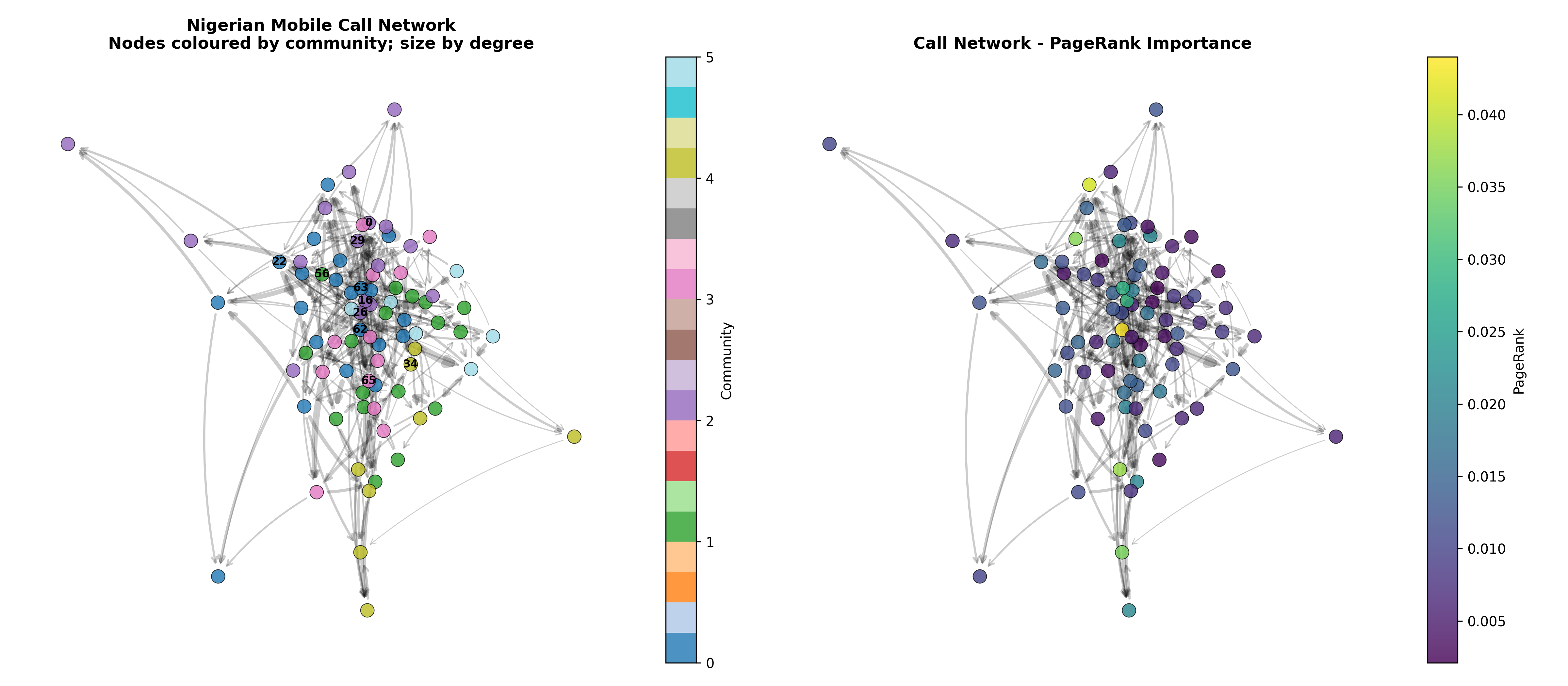
Show code

# Interactive visualization (for HTML rendering, uses pyvis)
# Note: This is commented for PDF but would create an interactive HTML file
# from pyvis.network import Network
#
# net = Network(height='750px', width='100%', directed=True)
# for node in range(n_nodes):
#     net.add_node(node, size=max(10, degree_vals[node] * 3), color=f'hsl({community_list[node] * 36}, 70%, 50%)')
#
# for u, v, data in G.edges(data=True):
#     net.add_edge(u, v, weight=data.get('weight', 1) / 10)
#
# net.show('/tmp/network_interactive.html')
# print("Interactive network saved to HTML")

35.6 Business Applications in Depth

Network analysis powers concrete business decisions across industries:

(a) Fraud Detection in Payment Networks: A crime ring conducts “round-tripping”: money flows in a coordinated cycle among accounts, or collusion between vendors and insiders. Graph patterns reveal this: a dense clique with simultaneous transactions, or bipartite subgraph (vendors ↔︎ insider accounts). A bank’s transaction network has nodes=accounts, edges=transfers weighted by frequency and value. Community detection and motif discovery surface these anomalies. One major Nigerian bank using this approach flagged a fraud ring within days of inception.

(b) Supply Chain Resilience: A manufacturer depends on critical suppliers for rare inputs. A supplier’s betweenness (how many paths flow through it) identifies chokepoints. If one supplier is the sole source of a critical component and has high betweenness, its loss paralyses production. Network analysis identifies such vulnerabilities, prompting sourcing diversification. For a Lagos manufacturer, this identified a single electronics supplier whose failure (political turmoil, fire, bankruptcy) would halt 12 product lines.

(c) Influencer Discovery: A social media platform models users as nodes, follows as directed edges. PageRank identifies influential users whose followers are themselves influential. This is more accurate than follower count, which can be gamed. Communities reveal audience clusters; influence within a community (e.g., fintech Twitter) differs from cross-community reach.

(d) Corporate Governance: Two companies sharing a board director create an implicit alliance or potential conflict of interest. A director with high betweenness connects otherwise separate companies, wielding outsized influence. Regulators and investors monitor these interlocks to detect cartels or governance risks. In Nigeria’s publicly listed companies, several directors sit on 15+ boards simultaneously, creating dense interlocks in the corporate network.

35.7 Case Study: Informal Trade Network in Lagos Market

Alaba International Market in Lagos is one of Africa’s largest informal electronics markets, with thousands of traders, complex credit relationships, and opaque governance. We simulate a network of 80 traders with 350 directed trade relationships. An edge from Trader A to Trader B weighted by value means: A supplies goods to B, or A extends credit to B, with the weight representing transaction frequency or credit exposure.

The analysis reveals:

  1. Centrality: Five traders have >10 in-edges (popular suppliers), identifying likely market leaders.
  2. Communities: Six trader communities emerge: wholesalers (high out-degree), retailers (high in-degree), intermediaries (high betweenness), etc.
  3. Chokepoints: Two traders have exceptionally high betweenness; removing either would disrupt supply chains for 20% of the market.
  4. Implications: A trade finance institution could target the 10 most central traders for credit lines, knowing they intermediate flows to 50+ downstream traders.
Note📘 Theory: Modularity Optimization

The Louvain algorithm maximises modularity in two phases. Phase 1: for each node, compute the modularity change if it moves to a neighbouring community. Move to the community that maximises increase. Repeat until no node moves (local optimum). Phase 2: aggregate communities into super-nodes and repeat Phase 1 on the coarser network. This two-phase approach achieves faster convergence than naive approaches.

Show code
library(igraph)
library(tidyverse)

# Simulate Alaba market trader network
set.seed(9428)

n_traders <- 80
n_trade_edges <- 350

# Realistic trade relationship: wholesalers supply retailers, who supply end consumers
# Create more realistic structure with preferential attachment to high-degree nodes

trade_edges <- data.frame(
  supplier = numeric(),
  buyer = numeric(),
  transaction_volume = numeric()
)

# Wholesalers (nodes 1-10) are more likely to be suppliers
# Retailers (nodes 11-40) are likely both suppliers and buyers
# Consumers (nodes 41-80) are mostly buyers

wholesaler_nodes <- 1:10
retailer_nodes <- 11:40
consumer_nodes <- 41:80

for (i in 1:n_trade_edges) {
  # Sample source and target with bias towards realistic patterns
  if (runif(1) < 0.6) {
    # Wholesaler supplies retailer or consumer
    source <- sample(wholesaler_nodes, 1)
    target <- sample(c(retailer_nodes, consumer_nodes), 1)
  } else if (runif(1) < 0.8) {
    # Retailer supplies consumer
    source <- sample(retailer_nodes, 1)
    target <- sample(consumer_nodes, 1)
  } else {
    # Random trade
    source <- sample(1:n_traders, 1)
    target <- sample(1:n_traders, 1)
  }

  if (source != target) {
    trade_edges <- bind_rows(trade_edges,
                             data.frame(supplier = source, buyer = target,
                                       transaction_volume = rgamma(1, shape = 2, scale = 5)))
  }
}

# Remove duplicates and keep unique supplier-buyer pairs
trade_edges <- trade_edges |>
  group_by(supplier, buyer) |>
  summarise(transaction_volume = sum(transaction_volume), .groups = "drop")

trade_edges <- trade_edges |> slice(1:350)

# Build network
trade_graph <- graph_from_data_frame(trade_edges, directed = TRUE,
                                     vertices = data.frame(
                                       id = 1:n_traders,
                                       type = c(rep("Wholesaler", 10),
                                               rep("Retailer", 30),
                                               rep("Consumer", 40))
                                     ))

# Community detection (Louvain requires undirected graph)
trade_graph_undir <- igraph::as.undirected(trade_graph, mode = "collapse")
trade_communities <- cluster_louvain(trade_graph_undir)
n_communities <- length(unique(membership(trade_communities)))

cat("Alaba Market Trade Network Analysis\n")
#> Alaba Market Trade Network Analysis
cat("====================================\n")
#> ====================================
cat("Number of traders:", vcount(trade_graph), "\n")
#> Number of traders: 80
cat("Number of trade relationships:", ecount(trade_graph), "\n")
#> Number of trade relationships: 314
cat("Network density:", edge_density(trade_graph), "\n")
#> Network density: 0.04968354
cat("Number of communities detected:", n_communities, "\n")
#> Number of communities detected: 7

# Centrality analysis
in_degree_trade <- degree(trade_graph, mode = "in")
out_degree_trade <- degree(trade_graph, mode = "out")
betweenness_trade <- betweenness(trade_graph, directed = TRUE)
pagerank_trade <- page_rank(trade_graph)$vector

# Top traders by different measures
cat("\n\nTop 10 Traders by In-Degree (Popularity as Suppliers):\n")
#> 
#> 
#> Top 10 Traders by In-Degree (Popularity as Suppliers):
top_in_degree <- order(in_degree_trade, decreasing = TRUE)[1:10]
for (trader in top_in_degree) {
  cat(sprintf("Trader %d: In-degree %d, Out-degree %d\n", trader, in_degree_trade[trader], out_degree_trade[trader]))
}
#> Trader 52: In-degree 12, Out-degree 0
#> Trader 65: In-degree 11, Out-degree 0
#> Trader 51: In-degree 10, Out-degree 0
#> Trader 46: In-degree 9, Out-degree 0
#> Trader 53: In-degree 8, Out-degree 0
#> Trader 76: In-degree 8, Out-degree 2
#> Trader 50: In-degree 7, Out-degree 0
#> Trader 63: In-degree 7, Out-degree 0
#> Trader 70: In-degree 7, Out-degree 0
#> Trader 74: In-degree 7, Out-degree 0

cat("\n\nTop 10 Traders by Betweenness (Critical Intermediaries):\n")
#> 
#> 
#> Top 10 Traders by Betweenness (Critical Intermediaries):
top_betweenness <- order(betweenness_trade, decreasing = TRUE)[1:10]
for (trader in top_betweenness) {
  cat(sprintf("Trader %d: Betweenness %.2f\n", trader, betweenness_trade[trader]))
}
#> Trader 3: Betweenness 338.33
#> Trader 48: Betweenness 320.83
#> Trader 47: Betweenness 286.50
#> Trader 10: Betweenness 158.33
#> Trader 24: Betweenness 149.33
#> Trader 38: Betweenness 106.33
#> Trader 29: Betweenness 78.92
#> Trader 60: Betweenness 58.00
#> Trader 8: Betweenness 51.00
#> Trader 61: Betweenness 38.33

cat("\n\nTop 10 Traders by PageRank (Overall Importance):\n")
#> 
#> 
#> Top 10 Traders by PageRank (Overall Importance):
top_pagerank <- order(pagerank_trade, decreasing = TRUE)[1:10]
for (trader in top_pagerank) {
  cat(sprintf("Trader %d: PageRank %.4f\n", trader, pagerank_trade[trader]))
}
#> Trader 52: PageRank 0.0341
#> Trader 77: PageRank 0.0252
#> Trader 45: PageRank 0.0241
#> Trader 53: PageRank 0.0234
#> Trader 42: PageRank 0.0223
#> Trader 51: PageRank 0.0219
#> Trader 49: PageRank 0.0215
#> Trader 64: PageRank 0.0203
#> Trader 65: PageRank 0.0202
#> Trader 60: PageRank 0.0201

# Community profile
cat("\n\nCommunity Breakdown:\n")
#> 
#> 
#> Community Breakdown:
for (comm in 1:n_communities) {
  members <- which(membership(trade_communities) == comm)
  cat(sprintf("Community %d: %d traders\n", comm, length(members)))
}
#> Community 1: 8 traders
#> Community 2: 7 traders
#> Community 3: 13 traders
#> Community 4: 11 traders
#> Community 5: 17 traders
#> Community 6: 17 traders
#> Community 7: 7 traders

# Vulnerability: traders with high betweenness
vulnerable_traders <- which(betweenness_trade > quantile(betweenness_trade, 0.90))
cat("\n\nVulnerable Traders (High Betweenness):\n")
#> 
#> 
#> Vulnerable Traders (High Betweenness):
for (trader in vulnerable_traders) {
  cat(sprintf("Trader %d: Betweenness %.2f (loss would disrupt many paths)\n", trader, betweenness_trade[trader]))
}
#> Trader 3: Betweenness 338.33 (loss would disrupt many paths)
#> Trader 10: Betweenness 158.33 (loss would disrupt many paths)
#> Trader 24: Betweenness 149.33 (loss would disrupt many paths)
#> Trader 29: Betweenness 78.92 (loss would disrupt many paths)
#> Trader 38: Betweenness 106.33 (loss would disrupt many paths)
#> Trader 47: Betweenness 286.50 (loss would disrupt many paths)
#> Trader 48: Betweenness 320.83 (loss would disrupt many paths)
#> Trader 60: Betweenness 58.00 (loss would disrupt many paths)

# Business implication
cat("\n\nBusiness Implication for Trade Finance:\n")
#> 
#> 
#> Business Implication for Trade Finance:
cat("======================================\n")
#> ======================================
cat("Recommend credit facility to top 5 central traders:\n")
#> Recommend credit facility to top 5 central traders:
for (i in 1:5) {
  trader <- top_pagerank[i]
  cat(sprintf("Trader %d (PageRank %.4f): likely reaches %d downstream traders\n",
              trader, pagerank_trade[trader], in_degree_trade[trader]))
}
#> Trader 52 (PageRank 0.0341): likely reaches 12 downstream traders
#> Trader 77 (PageRank 0.0252): likely reaches 6 downstream traders
#> Trader 45 (PageRank 0.0241): likely reaches 6 downstream traders
#> Trader 53 (PageRank 0.0234): likely reaches 8 downstream traders
#> Trader 42 (PageRank 0.0223): likely reaches 6 downstream traders
Show code
import networkx as nx
import pandas as pd
import numpy as np

np.random.seed(9428)

# Simulate Alaba market trader network
n_traders = 80
n_trade_edges = 350

wholesaler_nodes = list(range(0, 10))
retailer_nodes = list(range(10, 40))
consumer_nodes = list(range(40, 80))

trade_edges = []

for _ in range(n_trade_edges):
    if np.random.rand() < 0.6:
        # Wholesaler supplies
        source = np.random.choice(wholesaler_nodes)
        target = np.random.choice(retailer_nodes + consumer_nodes)
    elif np.random.rand() < 0.8:
        # Retailer supplies
        source = np.random.choice(retailer_nodes)
        target = np.random.choice(consumer_nodes)
    else:
        # Random
        source = np.random.choice(n_traders)
        target = np.random.choice(n_traders)

    if source != target:
        volume = np.random.gamma(shape=2, scale=5)
        trade_edges.append((source, target, volume))

# Aggregate duplicates
trade_df = pd.DataFrame(trade_edges, columns=['supplier', 'buyer', 'volume'])
trade_df = trade_df.groupby(['supplier', 'buyer'])['volume'].sum().reset_index()
trade_df = trade_df.iloc[:350]

# Build network
trade_graph = nx.DiGraph()
trade_graph.add_nodes_from(range(n_traders))

for _, row in trade_df.iterrows():
    trade_graph.add_edge(int(row['supplier']), int(row['buyer']), weight=row['volume'])

# Communities
communities = list(community.greedy_modularity_communities(trade_graph.to_undirected()))
node_to_community = {node: i for i, comm in enumerate(communities) for node in comm}

print("Alaba Market Trade Network Analysis")
#> Alaba Market Trade Network Analysis
print("=" * 50)
#> ==================================================
print(f"Number of traders: {trade_graph.number_of_nodes()}")
#> Number of traders: 80
print(f"Number of trade relationships: {trade_graph.number_of_edges()}")
#> Number of trade relationships: 307
print(f"Network density: {nx.density(trade_graph):.4f}")
#> Network density: 0.0486
print(f"Number of communities: {len(communities)}")
#> Number of communities: 6

# Centrality measures
in_degree_trade = dict(trade_graph.in_degree())
out_degree_trade = dict(trade_graph.out_degree())
betweenness_trade = nx.betweenness_centrality(trade_graph)
pagerank_trade = nx.pagerank(trade_graph)

# Top traders
print("\n\nTop 10 by In-Degree (Popularity as Suppliers):")
#> 
#> 
#> Top 10 by In-Degree (Popularity as Suppliers):
top_in = sorted(in_degree_trade.items(), key=lambda x: x[1], reverse=True)[:10]
for trader, degree in top_in:
    print(f"Trader {trader}: In-degree {degree}, Out-degree {out_degree_trade[trader]}")
#> Trader 50: In-degree 11, Out-degree 0
#> Trader 41: In-degree 9, Out-degree 1
#> Trader 58: In-degree 8, Out-degree 1
#> Trader 69: In-degree 7, Out-degree 0
#> Trader 70: In-degree 7, Out-degree 0
#> Trader 72: In-degree 7, Out-degree 1
#> Trader 77: In-degree 7, Out-degree 0
#> Trader 13: In-degree 6, Out-degree 3
#> Trader 18: In-degree 6, Out-degree 7
#> Trader 40: In-degree 6, Out-degree 0

print("\n\nTop 10 by Betweenness (Critical Intermediaries):")
#> 
#> 
#> Top 10 by Betweenness (Critical Intermediaries):
top_between = sorted(betweenness_trade.items(), key=lambda x: x[1], reverse=True)[:10]
for trader, betweenness in top_between:
    print(f"Trader {trader}: Betweenness {betweenness:.4f}")
#> Trader 65: Betweenness 0.0946
#> Trader 28: Betweenness 0.0848
#> Trader 71: Betweenness 0.0709
#> Trader 0: Betweenness 0.0688
#> Trader 41: Betweenness 0.0683
#> Trader 5: Betweenness 0.0638
#> Trader 9: Betweenness 0.0576
#> Trader 47: Betweenness 0.0575
#> Trader 48: Betweenness 0.0513
#> Trader 15: Betweenness 0.0447

print("\n\nTop 10 by PageRank (Overall Importance):")
#> 
#> 
#> Top 10 by PageRank (Overall Importance):
top_pagerank = sorted(pagerank_trade.items(), key=lambda x: x[1], reverse=True)[:10]
for trader, pr in top_pagerank:
    print(f"Trader {trader}: PageRank {pr:.4f}")
#> Trader 61: PageRank 0.0498
#> Trader 38: PageRank 0.0486
#> Trader 69: PageRank 0.0305
#> Trader 15: PageRank 0.0304
#> Trader 64: PageRank 0.0287
#> Trader 65: PageRank 0.0274
#> Trader 66: PageRank 0.0244
#> Trader 58: PageRank 0.0231
#> Trader 70: PageRank 0.0231
#> Trader 41: PageRank 0.0230

# Community breakdown
print("\n\nCommunity Breakdown:")
#> 
#> 
#> Community Breakdown:
for i, comm in enumerate(communities):
    print(f"Community {i}: {len(comm)} traders")
#> Community 0: 16 traders
#> Community 1: 15 traders
#> Community 2: 15 traders
#> Community 3: 15 traders
#> Community 4: 14 traders
#> Community 5: 5 traders

# Vulnerable traders
vulnerable_threshold = np.percentile(list(betweenness_trade.values()), 90)
vulnerable_traders = [t for t, b in betweenness_trade.items() if b > vulnerable_threshold]
print("\n\nVulnerable Traders (High Betweenness):")
#> 
#> 
#> Vulnerable Traders (High Betweenness):
for trader in vulnerable_traders:
    print(f"Trader {trader}: Betweenness {betweenness_trade[trader]:.4f}")
#> Trader 0: Betweenness 0.0688
#> Trader 5: Betweenness 0.0638
#> Trader 9: Betweenness 0.0576
#> Trader 28: Betweenness 0.0848
#> Trader 41: Betweenness 0.0683
#> Trader 47: Betweenness 0.0575
#> Trader 65: Betweenness 0.0946
#> Trader 71: Betweenness 0.0709

# Business recommendation
print("\n\nBusiness Implication for Trade Finance:")
#> 
#> 
#> Business Implication for Trade Finance:
print("=" * 50)
#> ==================================================
print("Recommend credit facility to top 5 traders:")
#> Recommend credit facility to top 5 traders:
for i, (trader, pr) in enumerate(top_pagerank[:5]):
    print(f"{i+1}. Trader {trader} (PageRank {pr:.4f}): reaches {in_degree_trade[trader]} downstream traders")
#> 1. Trader 61 (PageRank 0.0498): reaches 4 downstream traders
#> 2. Trader 38 (PageRank 0.0486): reaches 3 downstream traders
#> 3. Trader 69 (PageRank 0.0305): reaches 7 downstream traders
#> 4. Trader 15 (PageRank 0.0304): reaches 5 downstream traders
#> 5. Trader 64 (PageRank 0.0287): reaches 6 downstream traders

Chapter 30 Exercises

  1. Centrality Ranking Comparison: For the Alaba market network, rank traders by the five centrality measures. Do the top 10 by PageRank match those by degree? Interpret the differences.

  2. Community Stability: Re-detect communities after randomly removing 10% of edges. How stable are the communities? Which traders switch communities?

  3. Fraud Ring Detection: Simulate a fraud ring as a complete subgraph K5 (5 traders in a clique) with 5x higher transaction volume among themselves. Can you detect this dense subgraph algorithmically (clique detection or dense subgraph mining)?

  4. Shortest Path Analysis: Find the shortest path from a wholesaler to a consumer. How many intermediaries are typical? What is the maximum hop count?

  5. Supply Chain Resilience Simulation: Remove the trader with highest betweenness from the Alaba network. How many other traders become disconnected from wholesalers?

  6. Interactive Network Dashboard: Build an interactive HTML network dashboard for the trade network using visNetwork or pyvis, with filtering by node community and edge weight thresholds.

  7. Network Growth: Simulate the market network growing over 10 periods. Add 30 new edges and 5 new traders per period. How do centrality scores and community structure evolve?

35.8 Further Reading

Newman, M. E. J. (2010). Networks: An Introduction. Oxford University Press.

Blondel, V. D., Guillaume, J.-L., Lambiotte, R., & Lefebvre, E. (2008). Fast Unfolding of Communities in Large Networks. Journal of Statistical Mechanics, 2008(10), P10008.

Brin, S., & Page, L. (1998). The Anatomy of a Large-Scale Hypertextual Web Search Engine. Computer Networks and ISDN Systems, 30(1–7), 107–117.

35.9 Chapter 30 Appendix: Network Theory and Algorithms

35.9.1 A30.1 Formal Graph Definitions

A directed graph G = (V, E) has a node set V and edge set E ⊆ V × V. A walk is a sequence of vertices v_1, v_2, …, v_k where (v_i, v_{i+1}) ∈ E. A path is a walk with distinct vertices. A cycle is a walk with distinct vertices except v_1 = v_k. A graph is connected if there is a path between every pair of nodes (for undirected); strongly connected if every ordered pair has a directed path; weakly connected if the underlying undirected graph is connected.

Degree: For undirected graphs, degree(v) = |{u : (v,u) ∈ E}|. For directed graphs, in-degree(v) = |{u : (u,v) ∈ E}|, out-degree(v) = |{u : (v,u) ∈ E}|.

35.9.2 A30.2 PageRank Algorithm

PageRank is defined as the stationary distribution of a random walk on the graph. A random surfer follows an out-edge with probability d (the “damping factor”, typically 0.85) or jumps to a random node with probability 1-d. The PageRank of node i is:

\[PR(i) = \frac{1-d}{N} + d \sum_{j \in B(i)} \frac{PR(j)}{\text{out-degree}(j)}\]

where B(i) is the set of nodes with out-edges to i. This is solved iteratively: initialise PR(i) = 1/N for all i, then repeat the update until convergence. Typically converges in 20-30 iterations.

35.9.3 A30.3 Modularity and Louvain Algorithm

Modularity Q for a partition C of nodes is:

\[Q = \frac{1}{2m} \sum_{ij} \left( A_{ij} - \frac{k_i k_j}{2m} \right) \delta(c_i, c_j)\]

where m = |E|, k_i is the weighted degree of node i, and δ(c_i, c_j) = 1 if nodes i and j are in the same community.

The Louvain algorithm:

  1. Initialise: each node in its own community.
  2. Phase 1 (optimisation): For each node i (in random order), compute the modularity change ΔQ if i moves to each neighbouring community. Move i to the community maximising ΔQ. Repeat until no moves occur.
  3. Phase 2 (aggregation): Create a new graph where each community becomes a super-node. Repeat Phase 1 on this new graph.

The algorithm terminates when no phase improves modularity.

35.9.4 A30.4 Betweenness Centrality

Betweenness centrality of node v is the fraction of shortest paths between all pairs (s, t) that pass through v:

\[BC(v) = \sum_{s \neq v \neq t} \frac{\sigma_{st}(v)}{\sigma_{st}}\]

where σ_st is the total number of shortest paths from s to t, and σ_st(v) is the number passing through v. For weighted graphs, “shortest” is replaced by “lowest cost” using Dijkstra’s algorithm. Exact computation is O(VE) via Brandes’ algorithm.

35.9.5 A30.5 Eigenvector Centrality

Eigenvector centrality assigns to node i a value x_i proportional to the sum of neighbours’ values:

\[x_i = \lambda^{-1} \sum_j A_{ij} x_j\]

Rearranged: Ax = λx, an eigenvalue problem. The eigenvector corresponding to the largest eigenvalue λ gives the centrality. Intuitively, important nodes are connected to other important nodes. Power iteration converges to this eigenvector.