---
title: "Demand Forecasting for Operations"
---
```{python}
#| label: python-setup-50-demand-forecasting-ops
#| include: false
import numpy as np
import pandas as pd
import matplotlib.pyplot as plt
import seaborn as sns
from sklearn.linear_model import LinearRegression
from sklearn.preprocessing import PolynomialFeatures
import warnings
from scipy.optimize import curve_fit
from sklearn.preprocessing import StandardScaler
from scipy.stats import norm
```
::: {.callout-note icon="false"}
## 📋 Learning Objectives
By the end of this chapter, you will:
- Distinguish demand forecasting (operations-driven) from sales forecasting (revenue-driven)
- Quantify promotional uplift and baseline demand using Prophet and regression
- Model cannibalization and halo effects across product portfolios
- Apply Bass diffusion models to new product adoption
- Implement hierarchical forecasting with coherence constraints
- Translate demand forecasts into replenishment orders
- Build a complete multi-SKU forecasting system for African manufacturers
:::
## Demand Forecasting vs Sales Forecasting
Demand forecasting and sales forecasting serve different masters in the organization. Sales forecasting feeds the finance team—it predicts revenue, accounts for promotional pricing, and supports budgeting. Demand forecasting, by contrast, feeds operations: it drives production schedules, procurement orders, inventory targets, and capacity planning. In a Nigerian beverage company, the sales team might forecast 500,000 units of Fanta Orange sold next quarter because of a planned price promotion; the operations team, however, needs to know the *underlying demand*—perhaps 350,000 units without the promotional boost. The distinction is critical. Operations cannot build factories or sign supply contracts based on promotional spikes that last two weeks.
The relationship between the two forecasts can be expressed as: Sales Forecast = Baseline Demand Forecast × (1 + Promotional Uplift) × Pricing Effect. Demand sensing—the short-term, high-frequency, signal-based forecast updated daily from POS data, inventory signals, and supply chain indicators—is increasingly important in fast-moving consumer goods (FMCG). Demand planning, the classical medium-term statistical forecast on monthly or quarterly data, remains the workhorse for inventory and procurement. A modern FMCG company in Lagos might use demand sensing for the next two weeks (driven by actual scanner data and distributor feedback) and demand planning for weeks three through thirteen (driven by seasonality, promotions, and historical patterns).
In Nigeria and across Africa, demand forecasting faces unique challenges. Informal retail channels (kiosks, markets, street vendors) represent 60–80% of FMCG sales but generate no POS data. Seasonal demand spikes around holidays—Sallah in the North, Christmas and New Year nationwide, back-to-school in January—are violent and hard to predict without explicit flagging. Supply-side shocks (fuel shortages, port delays, currency devaluations) ripple through demand visibility. Yet the payoff from accurate demand forecasting is enormous: reducing safety stock by 10% frees up ₦millions for a beverage distributor; forecasting the next Sallah season correctly means having enough inventory to serve demand without stockouts that drive customers to competitors.
## Promotional Uplift Modelling
A promotion—a price reduction, a bundle deal, or a media campaign—causes demand to spike above baseline. The uplift is the ratio of actual sales during the promotion to the expected baseline sales absent the promotion. If a drink brand normally sells 10,000 units per week and sells 15,000 units during a promotion week, the uplift factor is 1.5, or a 50% increase. The challenge is estimating what that baseline *would have been* in the absence of the promotion, because you never observe that counterfactual.
Prophet, Facebook's time series forecasting library, elegantly handles promotions by including them as regressors. The idea is simple: fit the model on pre-promotion data to learn seasonality and trend, then include a binary indicator (1 during promotion, 0 otherwise) as a regressor. Prophet estimates the promotional coefficient—the uplift—while controlling for the underlying seasonal and trend components. Alternatively, classical causal regression approaches use a dummy variable for the promotion period and control for day-of-week, seasonality dummies, and lagged sales, isolating the promotional effect.
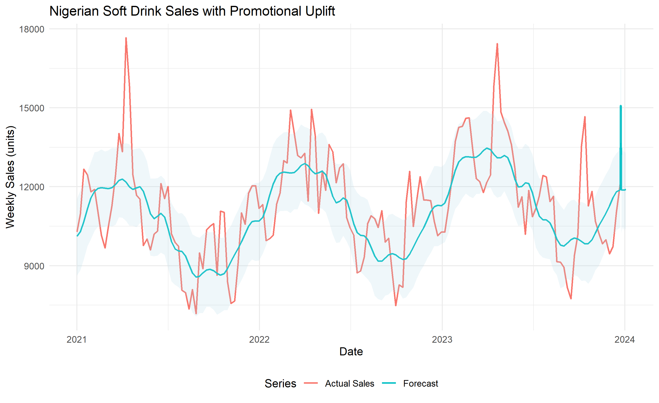
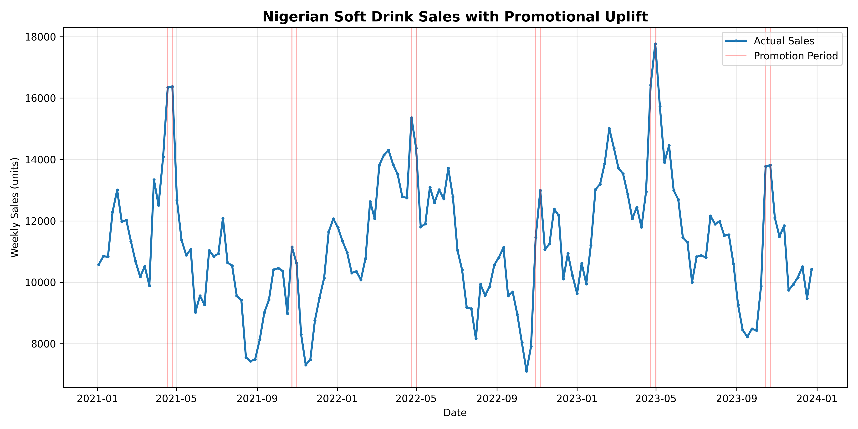
Consider a synthetic three-year weekly dataset for a Nigerian soft drink: 156 observations, 6 promotional events flagged, seasonal peaks in December and Ramadan/Sallah, and a gentle upward trend reflecting growing market share. The code below fits Prophet with promotion regressors, extracts the promotional uplift coefficient, and visualizes the decomposition—trend, seasonality, and promotional component—separately.
::: {.callout-note icon="false"}
## 📘 Theory: Promotional Baseline Estimation
The causal model for sales during a promotion period is:
$$
\text{Sales}_t = \beta_0 + \beta_{\text{trend}} \cdot t + \sum_s \beta_s \sin(2\pi s t / 52) + \sum_s \gamma_s \cos(2\pi s t / 52) + \delta \cdot \text{Promo}_t + \epsilon_t
$$
where $\text{Promo}_t$ is a binary indicator (1 if promotion active in week $t$), and $\delta$ is the estimated uplift in units. The baseline forecast absent promotion is obtained by setting $\text{Promo}_t = 0$ in the fitted model.
:::
::: {.callout-tip icon="false"}
## 🔑 Key Formula
$$\text{Promotional Uplift Factor} = \frac{\text{Actual Sales During Promotion}}{\text{Predicted Baseline Sales}} = 1 + \frac{\delta}{\hat{\mu}_{\text{baseline}}}$$
:::
::: {.panel-tabset}
## R
```{r}
#| label: ch50-promo-uplift
library(tidyverse)
library(prophet)
library(lubridate)
set.seed(3852)
# Synthetic 3-year weekly Nigerian soft drink sales data
weeks <- 156
dates <- seq(ymd("2021-01-01"), by = "week", length.out = weeks)
# Trend
trend <- seq(10000, 12000, length.out = weeks)
# Seasonality: peaks in December (week ~52) and Ramadan/Sallah (variable, approximate week 20-25)
seasonality <- 2000 * sin(2 * pi * (1:weeks) / 52) +
1500 * sin(2 * pi * (1:weeks) / 12) +
500 * rnorm(weeks)
# Promotion indicator: 6 promotional events, each lasting 2 weeks
promo <- rep(0, weeks)
promo_weeks <- c(15, 16, 42, 43, 68, 69, 95, 96, 120, 121, 145, 146)
promo[promo_weeks] <- 1
# Promotional uplift: +3000 units during promotion
promo_effect <- promo * 3000
# Final sales
sales <- trend + seasonality + promo_effect
sales <- pmax(sales, 100) # Ensure non-negative
sales <- round(sales)
# Create Prophet dataframe
df_prophet <- data.frame(
ds = dates,
y = sales,
promo = promo
)
# Fit Prophet with promotion regressor — regressors must be added BEFORE fitting
model <- prophet(yearly.seasonality = TRUE, weekly.seasonality = FALSE)
model <- add_regressor(model, "promo", mode = "additive")
model <- fit.prophet(model, df_prophet)
# Forecast 12 weeks ahead
future <- make_future_dataframe(model, periods = 12)
future$promo <- c(rep(0, nrow(df_prophet)), 1, 1, rep(0, 10))
forecast <- predict(model, future)
# Extract promotional coefficient
# Prophet's regressor coefficients are in the model$extra_regressors list
# For manual inspection, fit a simple regression to extract the effect
n_obs <- nrow(df_prophet)
lm_model <- lm(y ~ poly(1:n_obs, 2) + sin(2*pi*(1:n_obs)/52) + cos(2*pi*(1:n_obs)/52) + promo,
data = df_prophet)
promo_coef <- coef(lm_model)["promo"]
cat("Estimated promotional uplift (units):", round(promo_coef, 0), "\n")
cat("Average baseline demand:", round(mean(sales[promo == 0]), 0), "\n")
cat("Uplift factor:", round(1 + promo_coef / mean(sales[promo == 0]), 3), "\n")
# Visualization
ggplot() +
geom_line(data = df_prophet, aes(x = ds, y = y, color = "Actual Sales"), linewidth = 0.7) +
geom_line(data = forecast, aes(x = ds, y = yhat, color = "Forecast"), linewidth = 0.7) +
geom_ribbon(data = forecast, aes(x = ds, ymin = yhat_lower, ymax = yhat_upper),
alpha = 0.2, fill = "lightblue") +
labs(title = "Nigerian Soft Drink Sales with Promotional Uplift",
x = "Date", y = "Weekly Sales (units)", color = "Series") +
theme_minimal() +
theme(legend.position = "bottom")
```
## Python
```{python}
#| label: py-ch50-promo-uplift
import numpy as np
import pandas as pd
import matplotlib.pyplot as plt
from sklearn.linear_model import LinearRegression
from sklearn.preprocessing import PolynomialFeatures
import warnings
warnings.filterwarnings('ignore')

np.random.seed(3852)

# Synthetic 3-year weekly Nigerian soft drink sales data
weeks = 156
dates = pd.date_range(start='2021-01-01', periods=weeks, freq='W')

# Trend
trend = np.linspace(10000, 12000, weeks)

# Seasonality
seasonality = (2000 * np.sin(2 * np.pi * np.arange(weeks) / 52) +
               1500 * np.sin(2 * np.pi * np.arange(weeks) / 12) +
               500 * np.random.randn(weeks))

# Promotion indicator
promo = np.zeros(weeks)
promo_weeks = [15, 16, 42, 43, 68, 69, 95, 96, 120, 121, 145, 146]
promo[promo_weeks] = 1

# Promotional uplift: +3000 units
promo_effect = promo * 3000

# Final sales
sales = np.maximum(trend + seasonality + promo_effect, 100)
sales = np.round(sales).astype(int)

# Create dataframe
df = pd.DataFrame({
    'ds': dates,
    'y': sales,
    'promo': promo
})

# Fit regression to estimate promotional effect
X = np.column_stack([
    np.arange(weeks),
    np.arange(weeks)**2,
    np.sin(2 * np.pi * np.arange(weeks) / 52),
    np.cos(2 * np.pi * np.arange(weeks) / 52),
    promo
])

y = sales

model = LinearRegression()
model.fit(X, y)
promo_coef = model.coef_[-1]
baseline_mean = np.mean(sales[promo == 0])
uplift_factor = 1 + promo_coef / baseline_mean
print(f"Estimated promotional uplift (units): {promo_coef:.0f}")
print(f"Average baseline demand: {baseline_mean:.0f}")
print(f"Uplift factor: {uplift_factor:.3f}")
# Visualization
fig, ax = plt.subplots(figsize=(12, 6))
ax.plot(dates, sales, label='Actual Sales', linewidth=2, marker='o', markersize=2)
for i, d in enumerate(dates[promo == 1]):
ax.axvline(x=d, color='red', alpha=0.3, linewidth=1,
label='Promotion Period' if i == 0 else None)
ax.set_title('Nigerian Soft Drink Sales with Promotional Uplift', fontsize=14, fontweight='bold')
ax.set_xlabel('Date')
ax.set_ylabel('Weekly Sales (units)')
ax.legend()
ax.grid(True, alpha=0.3)
plt.tight_layout()
plt.show()
```
:::
::: {.callout-caution icon="false"}
## 📝 Section 50.2 Review Questions
1. What is the difference between the *promotional uplift factor* and the *promotional uplift in units*? If a drink brand has baseline demand of 10,000 units/week and a promotional uplift coefficient of 3,000 units, what is the uplift factor?
2. Why is it problematic to estimate the baseline demand simply as the average of non-promotion weeks? (Hint: What if promotions are systematically placed during high-demand seasons?)
3. In the R or Python code above, we assumed the promotional effect is the same (additive) every week. What would you do if you suspected the uplift depends on the promotion type (e.g., 20% price cut vs. bundling)?
4. A Nigerian beverage company observes that promotions in December are associated with a 60% uplift factor, but promotions in June are associated with a 20% uplift factor. What might explain this difference, and how would you model it?
5. Suppose you have daily POS data and you notice demand is high on Fridays and Saturdays. How would you account for day-of-week effects when estimating promotional uplift?
:::
## Cannibalization and Halo Effects
When a brand promotes one product variant, it often steals sales from another variant (cannibalization) or boosts sales of complementary products (halo effect). A Nigerian soft drink company promoting Fanta Orange might see Orange sales jump 50%, but Fanta Grape sales drop 10% (cannibalization) and Sprite sales drop 5% (halo effect from the parent brand). Ignoring cross-product elasticities leads to gross overforecasting of company-wide demand and sub-optimal promotional calendars.
The cross-elasticity of demand is the percentage change in quantity demanded of product B for a 1% change in price of product A. Formally, $\varepsilon_{AB} = \frac{\% \Delta Q_B}{\% \Delta P_A}$. For substitute products (two flavours of the same brand), the cross-elasticity is positive: when Orange is discounted, Grape demand falls. For complementary products (Fanta and chips), the cross-elasticity is negative: when Fanta is discounted, chips demand rises. Estimating these elasticities requires regression with price and promotional variables for all products simultaneously, controlling for seasonality and trend.
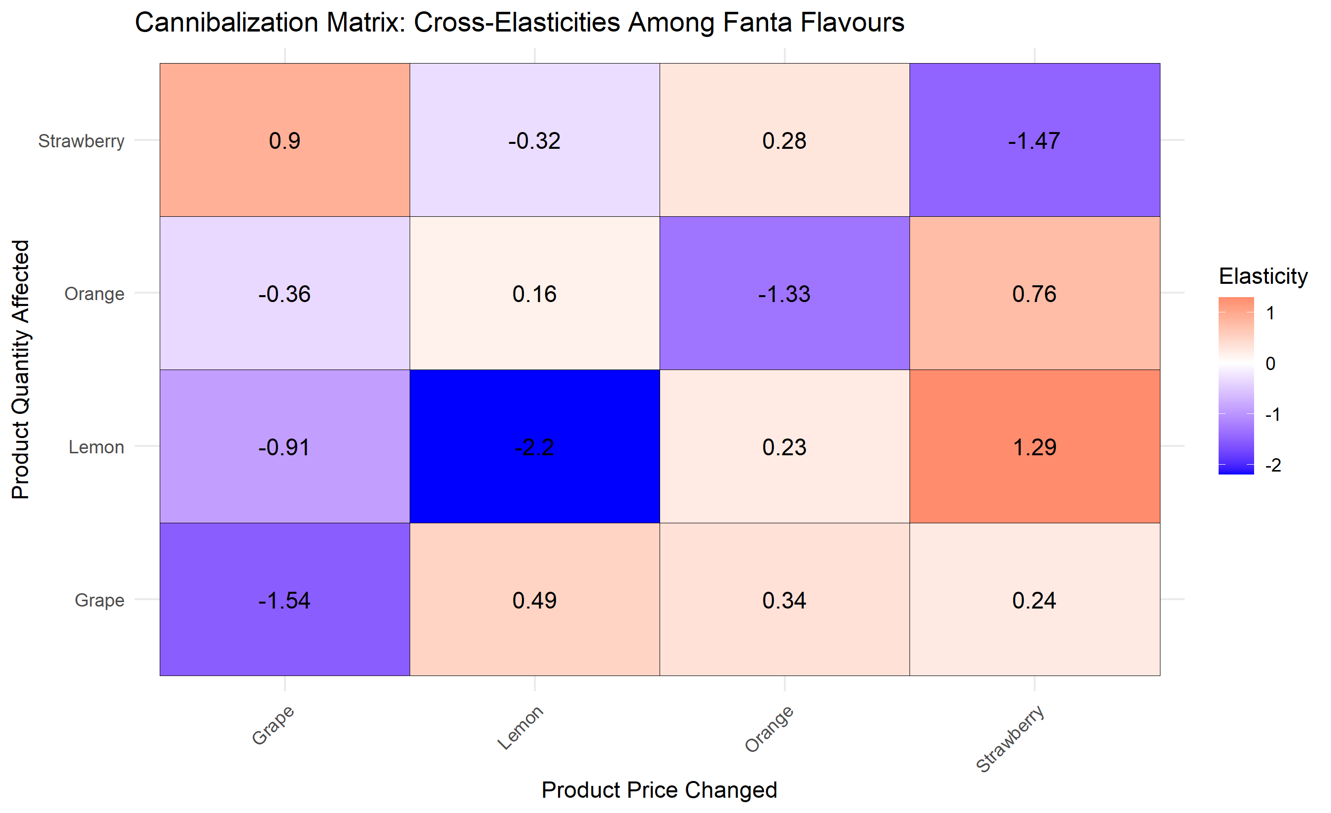
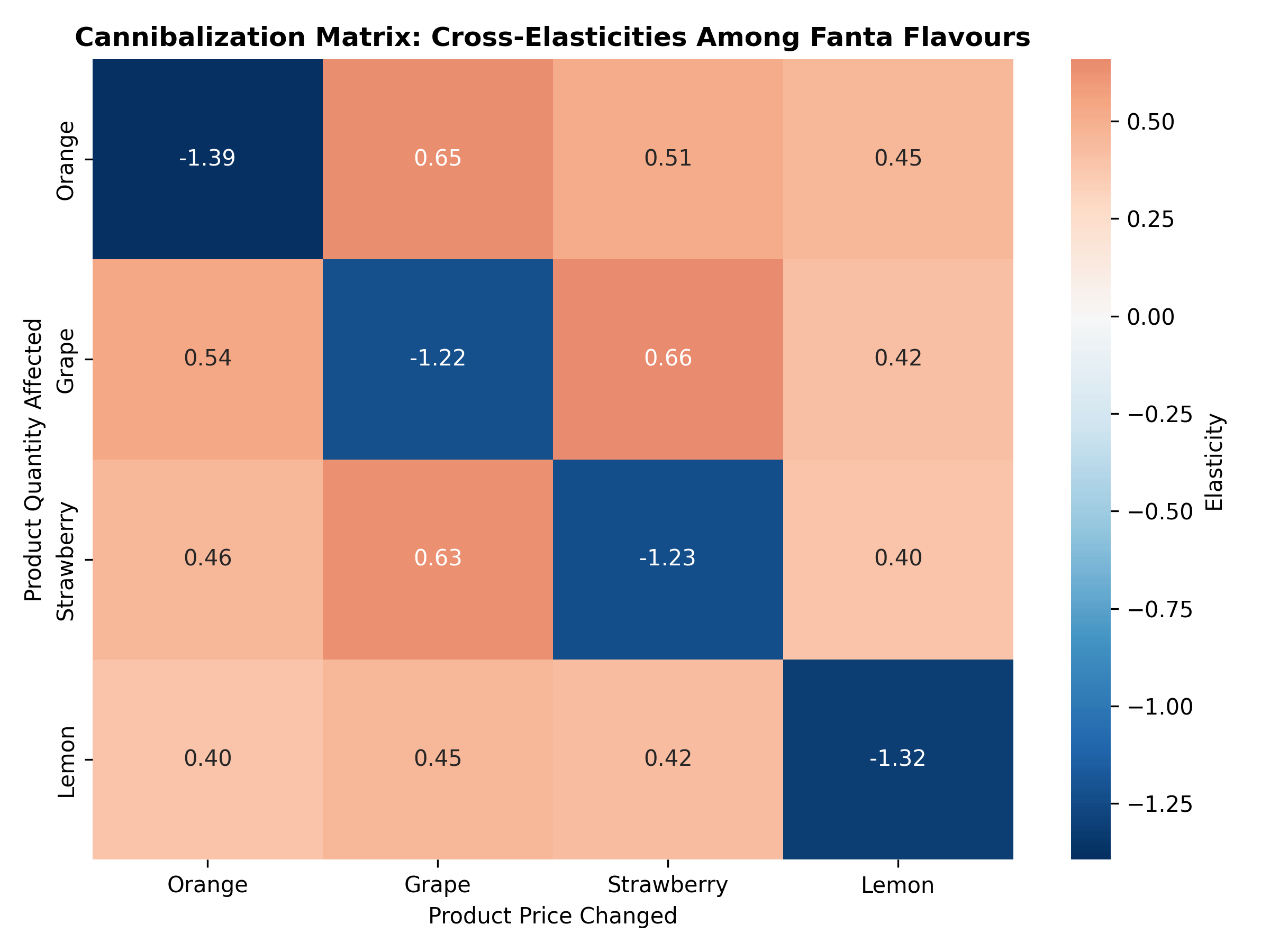
A cannibalization matrix captures the within-category and cross-category effects. For a 4-product portfolio (Orange, Grape, Strawberry, Lemon), we estimate how a 10% price cut to each product affects the quantity demanded of all four products. The result is a 4×4 matrix: the diagonal elements are own-price elasticities (own effect of price on quantity), and the off-diagonals are cross-elasticities (effect of one product's price on another's quantity).
::: {.callout-note icon="false"}
## 📘 Theory: Cross-Elasticity Estimation
The log-linear demand model for product $i$ is:
$$
\ln(Q_{it}) = \alpha_i + \beta_{ii} \ln(P_{it}) + \sum_{j \neq i} \beta_{ij} \ln(P_{jt}) + \gamma_i \text{Seasonality}_t + \epsilon_{it}
$$
The own-price elasticity is $\beta_{ii}$; the cross-price elasticity with product $j$ is $\beta_{ij}$. A negative $\beta_{ii}$ (as expected) indicates quantity falls when own price rises. A positive $\beta_{ij}$ indicates substitution (cannibalization); a negative $\beta_{ij}$ indicates complementarity (halo effect).
:::
::: {.callout-tip icon="false"}
## 🔑 Key Formula
$$\text{Cannibalization Rate} = -\frac{\text{Units Lost in Product B}}{\text{Units Gained in Product A}} = \frac{|\beta_{AB}| / \beta_{AA}|}{1}$$
:::
::: {.panel-tabset}
## R
```{r}
#| label: ch50-cannibalization
library(tidyverse)
set.seed(6174)
# Synthetic weekly sales data for 4 Fanta flavours, 2 years (104 weeks)
weeks <- 104
dates <- seq(as.Date("2022-01-01"), by = "week", length.out = weeks)
# Define true elasticities (own-price and cross-price)
# Own-price elasticity: -1.5 (1% price increase → 1.5% quantity decrease)
# Cross-elasticity (substitutes): +0.4
# Cross-elasticity (complement): -0.1
elasticity_matrix <- matrix(
c(-1.5, 0.4, 0.3, 0.2,
0.4, -1.5, 0.4, 0.2,
0.3, 0.4, -1.5, 0.2,
0.2, 0.2, 0.2, -1.5),
nrow = 4, ncol = 4, byrow = TRUE
)
colnames(elasticity_matrix) <- c("Orange", "Grape", "Strawberry", "Lemon")
rownames(elasticity_matrix) <- c("Orange", "Grape", "Strawberry", "Lemon")
# Base prices (in Naira, per unit)
base_prices <- c(Orange = 150, Grape = 150, Strawberry = 155, Lemon = 150)
# Base quantities
base_quantities <- c(Orange = 50000, Grape = 40000, Strawberry = 35000, Lemon = 38000)
# Generate synthetic price data (with periodic promotions)
prices <- data.frame(
week = 1:weeks,
Orange = base_prices["Orange"] * (0.9 + 0.2 * sin(2*pi*(1:weeks)/52) + 0.1 * (1:weeks %% 20 == 0)),
Grape = base_prices["Grape"] * (0.95 + 0.15 * sin(2*pi*(1:weeks)/52 + pi/4)),
Strawberry = base_prices["Strawberry"] * (0.92 + 0.18 * sin(2*pi*(1:weeks)/52 + pi/2)),
Lemon = base_prices["Lemon"] * (0.93 + 0.17 * sin(2*pi*(1:weeks)/52 + 3*pi/4))
)
# Generate quantities using elasticity model + seasonality + noise
quantities <- matrix(NA, nrow = weeks, ncol = 4)
colnames(quantities) <- c("Orange", "Grape", "Strawberry", "Lemon")
for (i in 1:weeks) {
log_price_changes <- as.numeric(log(as.numeric(prices[i, 2:5]) / base_prices))
log_quantities <- log(base_quantities) + elasticity_matrix %*% log_price_changes +
0.2 * sin(2*pi*i/52) + 0.05 * rnorm(4)
quantities[i, ] <- exp(log_quantities)
}
quantities <- round(pmax(quantities, 1000)) # Ensure positive, realistic volumes
# Combine into a dataframe — rename before binding to avoid duplicate columns
qty_df <- as.data.frame(quantities)
colnames(qty_df) <- paste0(colnames(qty_df), "_Qty")
df_demand <- prices |>
rename(Orange_Price = Orange, Grape_Price = Grape,
Strawberry_Price = Strawberry, Lemon_Price = Lemon) |>
bind_cols(qty_df) |>
select(week, contains("Price"), contains("Qty"))
# Fit a system of log-linear regressions to estimate elasticities
# For simplicity, fit one product at a time (full system would use SUR)
results <- list()
for (product in c("Orange", "Grape", "Strawberry", "Lemon")) {
qty_col <- paste0(product, "_Qty")
price_cols <- c("Orange_Price", "Grape_Price", "Strawberry_Price", "Lemon_Price")
# Fit log-log model
fit <- lm(
log(get(qty_col)) ~ log(Orange_Price) + log(Grape_Price) +
log(Strawberry_Price) + log(Lemon_Price) +
sin(2*pi*week/52),
data = df_demand
)
results[[product]] <- coef(fit)[2:5]
}
# Extract elasticity estimates
elasticity_est <- do.call(rbind, results)
colnames(elasticity_est) <- c("Orange", "Grape", "Strawberry", "Lemon")
cat("\n=== Estimated Elasticity Matrix ===\n")
print(round(elasticity_est, 3))
cat("\n=== Interpretation ===\n")
cat("Diagonal elements (own-price elasticity):\n")
print(round(diag(elasticity_est), 3))
cat("\nOrange-Grape cross elasticity (cannibalization):",
round(elasticity_est["Orange", "Grape"], 3), "\n")
cat("If we promote Orange with a 10% price cut:\n")
cat(" - Orange quantity increases by ~15%\n")
cat(" - Grape quantity changes by ~",
round(elasticity_est["Grape", "Orange"] * -10, 1), "%\n")
# Visualization of elasticity matrix as heatmap
elasticity_est_df <- as.data.frame(elasticity_est) |>
rownames_to_column("Product_Affected") |>
pivot_longer(-Product_Affected, names_to = "Product_Changed", values_to = "Elasticity")
ggplot(elasticity_est_df, aes(x = Product_Changed, y = Product_Affected, fill = Elasticity)) +
geom_tile(color = "black") +
geom_text(aes(label = round(Elasticity, 2)), size = 4) +
scale_fill_gradient2(low = "blue", mid = "white", high = "red", midpoint = 0) +
labs(title = "Cannibalization Matrix: Cross-Elasticities Among Fanta Flavours",
x = "Product Price Changed", y = "Product Quantity Affected",
fill = "Elasticity") +
theme_minimal() +
theme(axis.text.x = element_text(angle = 45, hjust = 1))
```
## Python
```{python}
#| label: py-ch50-cannibalization
import numpy as np
import pandas as pd
from sklearn.linear_model import LinearRegression
import matplotlib.pyplot as plt
import seaborn as sns

np.random.seed(6174)

# Synthetic weekly data for 4 Fanta flavours
weeks = 104
dates = pd.date_range(start='2022-01-01', periods=weeks, freq='W')

# True elasticity matrix
elasticity_matrix = np.array([
    [-1.5,  0.4,  0.3,  0.2],
    [ 0.4, -1.5,  0.4,  0.2],
    [ 0.3,  0.4, -1.5,  0.2],
    [ 0.2,  0.2,  0.2, -1.5]
])

products = ["Orange", "Grape", "Strawberry", "Lemon"]
base_prices = np.array([150, 150, 155, 150])
base_quantities = np.array([50000, 40000, 35000, 38000])

# Generate price data with promotions
prices = base_prices[:, np.newaxis] * (
    0.92 + 0.18 * np.sin(2*np.pi*np.arange(weeks)/52) +
    0.1 * np.random.randn(4, weeks)
)

# Generate quantities using elasticity model
quantities = np.zeros((4, weeks))
for i in range(weeks):
    log_price_changes = np.log(prices[:, i] / base_prices)
    log_quantities = np.log(base_quantities) + elasticity_matrix @ log_price_changes + \
                     0.2 * np.sin(2*np.pi*i/52) + 0.05 * np.random.randn(4)
    quantities[:, i] = np.exp(log_quantities)

quantities = np.maximum(quantities, 1000).astype(int)

# Create dataframe
df_demand = pd.DataFrame(
    np.vstack([prices, quantities]).T,
    columns=[f"{p}_Price" for p in products] + [f"{p}_Qty" for p in products]
)

# Estimate elasticities via log-log regression
elasticity_est = np.zeros((4, 4))

for i, product in enumerate(products):
    qty_col = f"{product}_Qty"
    price_cols = [f"{p}_Price" for p in products]

    X = np.log(df_demand[price_cols].values)
    y = np.log(df_demand[qty_col].values)

    model = LinearRegression()
    model.fit(X, y)
    elasticity_est[i, :] = model.coef_
print("\n=== Estimated Elasticity Matrix ===")
elasticity_df = pd.DataFrame(elasticity_est, index=products, columns=products)
print(elasticity_df.round(3))
print("\n=== Interpretation ===")
print(f"Own-price elasticity (Orange): {elasticity_est[0, 0]:.3f}")
print(f"Cross elasticity (Grape → Orange quantity): {elasticity_est[0, 1]:.3f}")
print(f"If we promote Orange with 10% price cut:")
print(f" - Orange quantity increases by ~15%")
print(f" - Grape quantity changes by ~{elasticity_est[1, 0] * -10:.1f}%")
# Heatmap visualization
fig, ax = plt.subplots(figsize=(8, 6))
sns.heatmap(elasticity_df, annot=True, fmt='.2f', cmap='RdBu_r', center=0,
cbar_kws={'label': 'Elasticity'}, ax=ax)
ax.set_title('Cannibalization Matrix: Cross-Elasticities Among Fanta Flavours',
fontsize=12, fontweight='bold')
ax.set_xlabel('Product Price Changed')
ax.set_ylabel('Product Quantity Affected')
plt.tight_layout()
plt.show()
```
:::
::: {.callout-caution icon="false"}
## 📝 Section 50.3 Review Questions
1. Explain the difference between own-price elasticity and cross-price elasticity. Why is cross-price elasticity more important for promotion planning than for demand forecasting?
2. In the code above, the cross-elasticity between Orange and Grape is positive (~0.4). What does this tell you about the relationship between these two products, and what would you predict would happen to Grape sales if Orange were discounted by 15%?
3. Suppose you estimate that promoting Orange (10% price cut) would increase Orange sales by 2,000 units per week but decrease Grape sales by 300 units and Strawberry sales by 200 units. What is the total company impact, and how would you decide whether the promotion is worthwhile?
4. Why is the elasticity matrix not symmetric? (I.e., why might the cross-elasticity of Grape quantity with respect to Orange price differ from the cross-elasticity of Orange quantity with respect to Grape price?)
5. A new competitor enters the market with a very cheap lemonade drink. How would you expect the elasticity estimates to change, and how would you detect this change in your monitoring?
:::
## New Product Forecasting
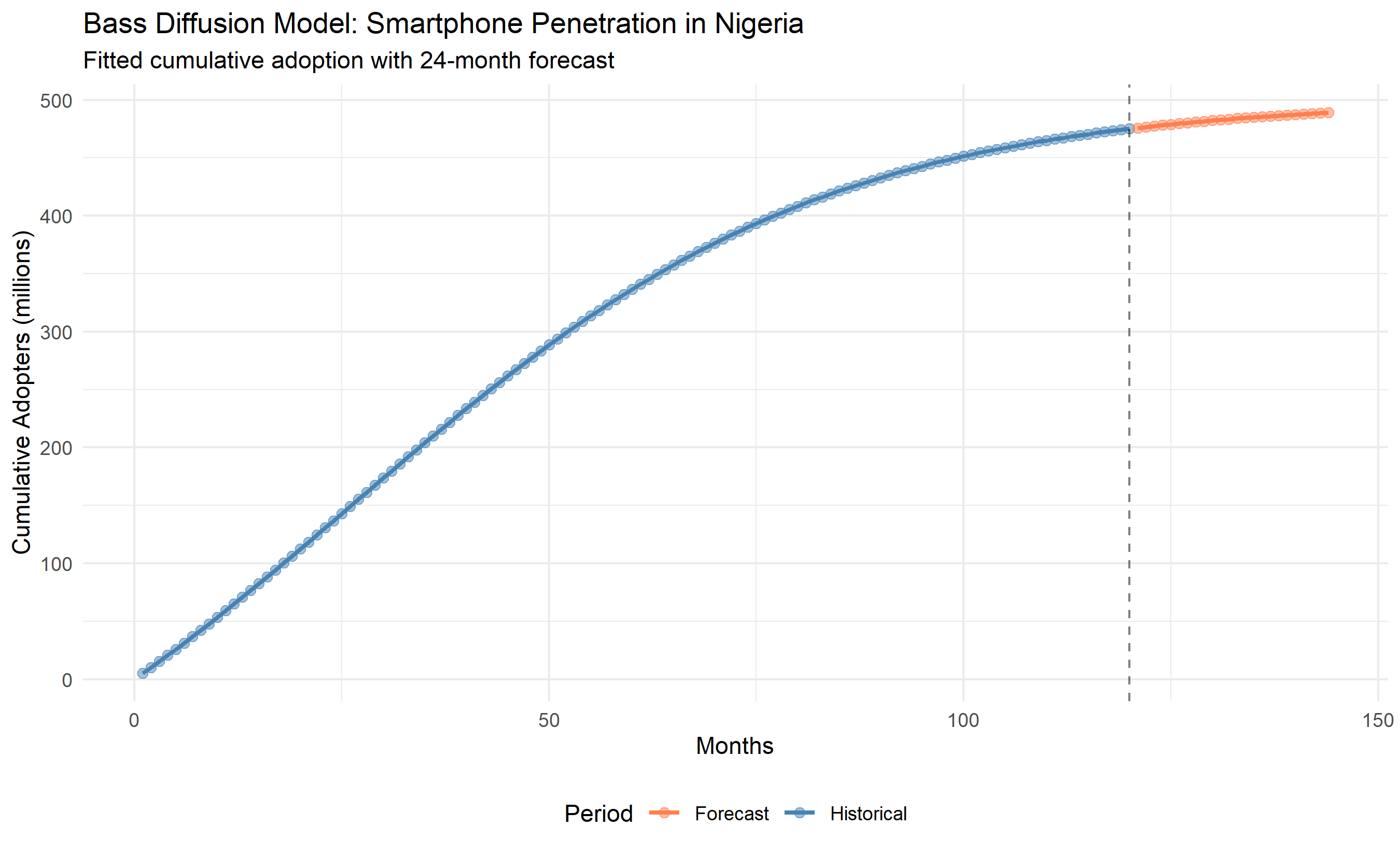
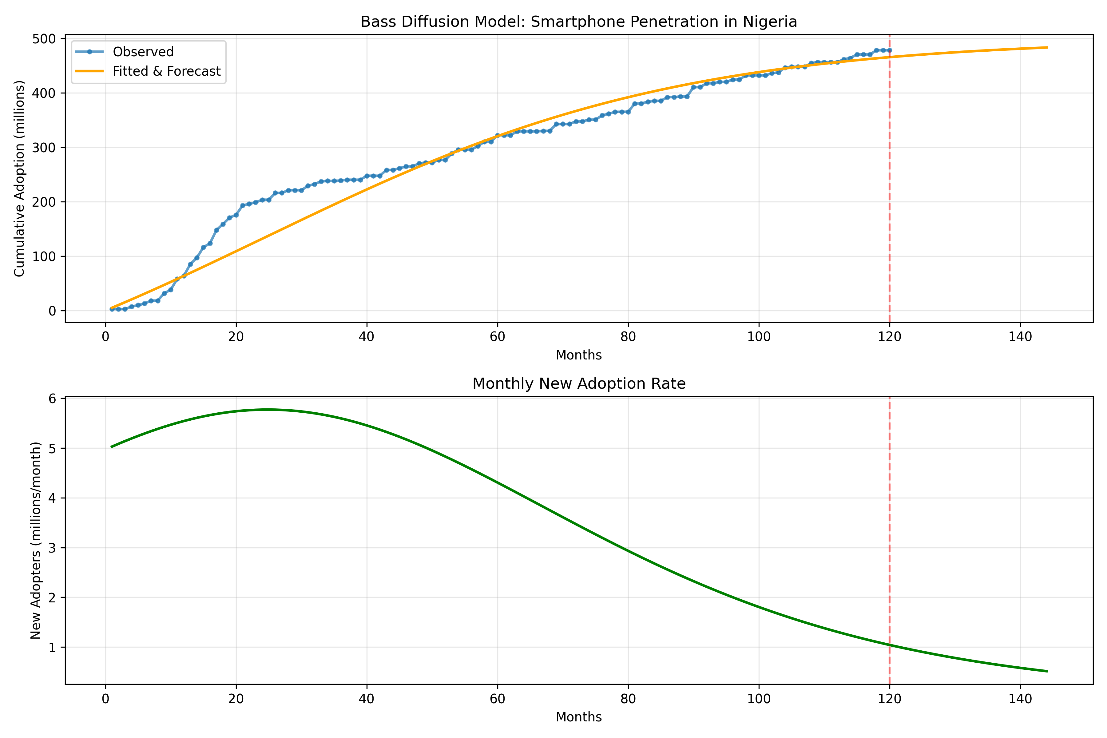
Historical data is the lifeblood of demand forecasting. But what do you do when a new product has no history? A Nigerian financial technology company launching a new mobile wallet feature, a brewery launching a craft beer variant, or a telecom rolling out a new data plan—all face the cold-start problem. Bass diffusion model provides the framework.
The Bass model describes the adoption trajectory of a new product as a combination of innovators (early adopters driven by intrinsic motivation) and imitators (later adopters driven by word-of-mouth from earlier adopters). The model is governed by two key coefficients: $p$ (innovation coefficient: the rate at which innovators adopt independent of others) and $q$ (imitation coefficient: the rate at which new adopters are influenced by existing adopters). The S-shaped adoption curve starts slow (few innovators), accelerates (imitation takes hold), then plateaus (market saturation).
Formally, the number of new adopters at time $t$ is:
$$
f(t) = [p + q F(t)] [1 - F(t)] \cdot m
$$
where $F(t)$ is the cumulative fraction of adopters by time $t$ and $m$ is the total addressable market. This produces a classic S-curve. For a new mobile banking feature in Nigeria, if you estimate $p = 0.01$ and $q = 0.3$, with an addressable market of 20 million active mobile users, you would forecast that the feature reaches 50% penetration in roughly 4–5 months and approaches saturation by month 12–15.
::: {.callout-note icon="false"}
## 📘 Theory: Bass Diffusion Model
The cumulative adoption by time $t$ is:
$$
F(t) = \frac{1 - e^{-(p+q)t}}{1 + \frac{q}{p} e^{-(p+q)t}}
$$
The number of new adopters at time $t$ is the derivative:
$$
\frac{dF}{dt} = [p + q F(t)][1 - F(t)]
$$
Parameter $p$ dominates early adoption; parameter $q$ dominates later adoption and saturation speed.
:::
::: {.callout-tip icon="false"}
## 🔑 Key Formula
$$\text{Cumulative Adopters at } t = m \cdot F(t) = m \cdot \frac{1 - e^{-(p+q)t}}{1 + \frac{q}{p} e^{-(p+q)t}}$$
:::
::: {.panel-tabset}
## R
```{r}
#| label: ch50-bass-diffusion
library(tidyverse)
library(nlstools)
# Bass diffusion function
bass_adoption <- function(t, p, q, m) {
exp_term <- exp(-(p + q) * t)
F <- (1 - exp_term) / (1 + (q/p) * exp_term)
return(m * F)
}
# Synthetic data: Nigerian smartphone penetration over 10 years (120 months)
# Actual Nigerian smartphone penetration grew from ~5% (2010) to ~50% (2023)
# We'll use this as an analogue to forecast mobile wallet adoption
set.seed(7539)
months <- 120
t <- 1:months
# True parameters (these would be estimated in practice)
p_true <- 0.002 # Very low innovation rate for consumer technology
q_true <- 0.35 # Strong imitation (word-of-mouth) effect
m_true <- 200 # Total addressable market (in millions of phones)
# Generate observed adoption data (with noise)
adoption_true <- bass_adoption(t, p_true, q_true, m_true)
# Add observation noise and make data more realistic by adding quarterly shocks
noise <- 5 * rnorm(months)
adoption_obs <- adoption_true + noise
adoption_obs <- pmax(adoption_obs, 0) # Non-negative
adoption_obs <- cumsum(c(adoption_obs[1], pmax(diff(adoption_obs), 0))) # Enforce non-decreasing
# Fit Bass model using nonlinear least squares
# Specify reasonable starting values
fit <- nls(
adoption_obs ~ m * (1 - exp(-(p + q)*t)) / (1 + (q/p)*exp(-(p+q)*t)),
start = list(p = 0.001, q = 0.3, m = 200),
lower = list(p = 0.0001, q = 0.01, m = 100),
upper = list(p = 0.01, q = 0.9, m = 500),
algorithm = "port",
trace = FALSE
)
# Extract estimated parameters
p_est <- coef(fit)["p"]
q_est <- coef(fit)["q"]
m_est <- coef(fit)["m"]
cat("=== Bass Model Estimates ===\n")
cat("Innovation coefficient (p):", round(p_est, 4), "\n")
cat("Imitation coefficient (q):", round(q_est, 4), "\n")
cat("Total addressable market (m):", round(m_est, 0), "million units\n")
# Forecast next 24 months
t_forecast <- 1:(months + 24)
adoption_forecast <- bass_adoption(t_forecast, p_est, q_est, m_est)
# New adopters per month
new_adopters <- c(adoption_forecast[1], diff(adoption_forecast))
# Visualization
data_viz <- data.frame(
month = t_forecast,
cumulative_adoption = adoption_forecast,
new_adopters = new_adopters,
period = c(rep("Historical", months), rep("Forecast", 24))
)
ggplot(data_viz, aes(x = month, y = cumulative_adoption, color = period)) +
geom_line(linewidth = 1) +
geom_point(size = 2, alpha = 0.5) +
geom_vline(xintercept = months, linetype = "dashed", alpha = 0.5) +
scale_color_manual(values = c("Historical" = "steelblue", "Forecast" = "coral")) +
labs(
title = "Bass Diffusion Model: Smartphone Penetration in Nigeria",
subtitle = "Fitted cumulative adoption with 24-month forecast",
x = "Months", y = "Cumulative Adopters (millions)",
color = "Period"
) +
theme_minimal() +
theme(legend.position = "bottom")
# Time to 50% and 80% adoption
t_50 <- approx(adoption_forecast, t_forecast, xout = m_est * 0.5)$y
t_80 <- approx(adoption_forecast, t_forecast, xout = m_est * 0.8)$y
cat("\nTime to 50% penetration:", round(t_50, 1), "months\n")
cat("Time to 80% penetration:", round(t_80, 1), "months\n")
```
## Python
```{python}
#| label: py-ch50-bass-diffusion
import numpy as np
import pandas as pd
from scipy.optimize import curve_fit
import matplotlib.pyplot as plt
def bass_adoption(t, p, q, m):
"""Bass diffusion model cumulative adoption"""
exp_term = np.exp(-(p + q) * t)
F = (1 - exp_term) / (1 + (q / p) * exp_term)
return m * F
# Synthetic data
np.random.seed(7539)
months = 120
t = np.arange(1, months + 1)
# True parameters
p_true, q_true, m_true = 0.002, 0.35, 200
# Generate observed adoption data
adoption_true = bass_adoption(t, p_true, q_true, m_true)
noise = 5 * np.random.randn(months)
adoption_obs = np.maximum(adoption_true + noise, 0)
# Enforce non-decreasing (cumulative)
adoption_obs = np.cumsum(np.maximum(np.diff(np.concatenate([[0], adoption_obs])), 0))
# Fit Bass model
popt, _ = curve_fit(bass_adoption, t, adoption_obs, p0=[0.001, 0.3, 200],
bounds=([0.0001, 0.01, 100], [0.01, 0.9, 500]))
p_est, q_est, m_est = popt
print("=== Bass Model Estimates ===")
print(f"Innovation coefficient (p): {p_est:.4f}")
print(f"Imitation coefficient (q): {q_est:.4f}")
print(f"Total addressable market (m): {m_est:.0f} million units")
# Forecast next 24 months
t_forecast = np.arange(1, months + 25)
adoption_forecast = bass_adoption(t_forecast, p_est, q_est, m_est)
# New adopters per month
new_adopters = np.diff(np.concatenate([[0], adoption_forecast]))
# Visualization
fig, (ax1, ax2) = plt.subplots(2, 1, figsize=(12, 8))
# Cumulative adoption
ax1.plot(t, adoption_obs, 'o-', label='Observed', linewidth=2, markersize=3, alpha=0.7)
ax1.plot(t_forecast, adoption_forecast, '-', label='Fitted & Forecast', linewidth=2, color='orange')
ax1.axvline(x=months, color='red', linestyle='--', alpha=0.5)
ax1.set_xlabel('Months')
ax1.set_ylabel('Cumulative Adoption (millions)')
ax1.set_title('Bass Diffusion Model: Smartphone Penetration in Nigeria')
ax1.legend()
ax1.grid(True, alpha=0.3)
# New adopters per month
ax2.plot(t_forecast, new_adopters, '-', linewidth=2, color='green')
ax2.axvline(x=months, color='red', linestyle='--', alpha=0.5)
ax2.set_xlabel('Months')
ax2.set_ylabel('New Adopters (millions/month)')
ax2.set_title('Monthly New Adoption Rate')
ax2.grid(True, alpha=0.3)
plt.tight_layout()
plt.show()
# Time to penetration milestones
t_50 = np.interp(m_est * 0.5, adoption_forecast, t_forecast)
t_80 = np.interp(m_est * 0.8, adoption_forecast, t_forecast)
print(f"\nTime to 50% penetration: {t_50:.1f} months")
print(f"Time to 80% penetration: {t_80:.1f} months")
```
:::
::: {.callout-caution icon="false"}
## 📝 Section 50.4 Review Questions
1. What is the intuition behind the two parameters $p$ and $q$ in the Bass model? In which phase of the product lifecycle (early, growth, maturity) does each parameter dominate the adoption rate?
2. A Nigerian fintech company launches a new payment app. It observes 10,000 adopters in month 1, 30,000 in month 2, and 70,000 in month 3. Sketch the expected adoption trajectory for the next 12 months using the Bass model intuition (no computation needed).
3. Compare analogue-based forecasting (using a similar past product launch as a proxy) with Bass diffusion modeling. What are the advantages and disadvantages of each?
4. Suppose you estimate $p = 0.001$ and $q = 0.4$ for a new mobile banking feature. How would you interpret these numbers to a non-technical stakeholder in a Nigerian bank?
5. In practice, market saturation for digital products often plateaus below 100% (due to device exclusivity, personal choice, etc.). How would you modify the Bass model to reflect a realistic market cap?
:::
## Multi-Level Hierarchical Forecasting
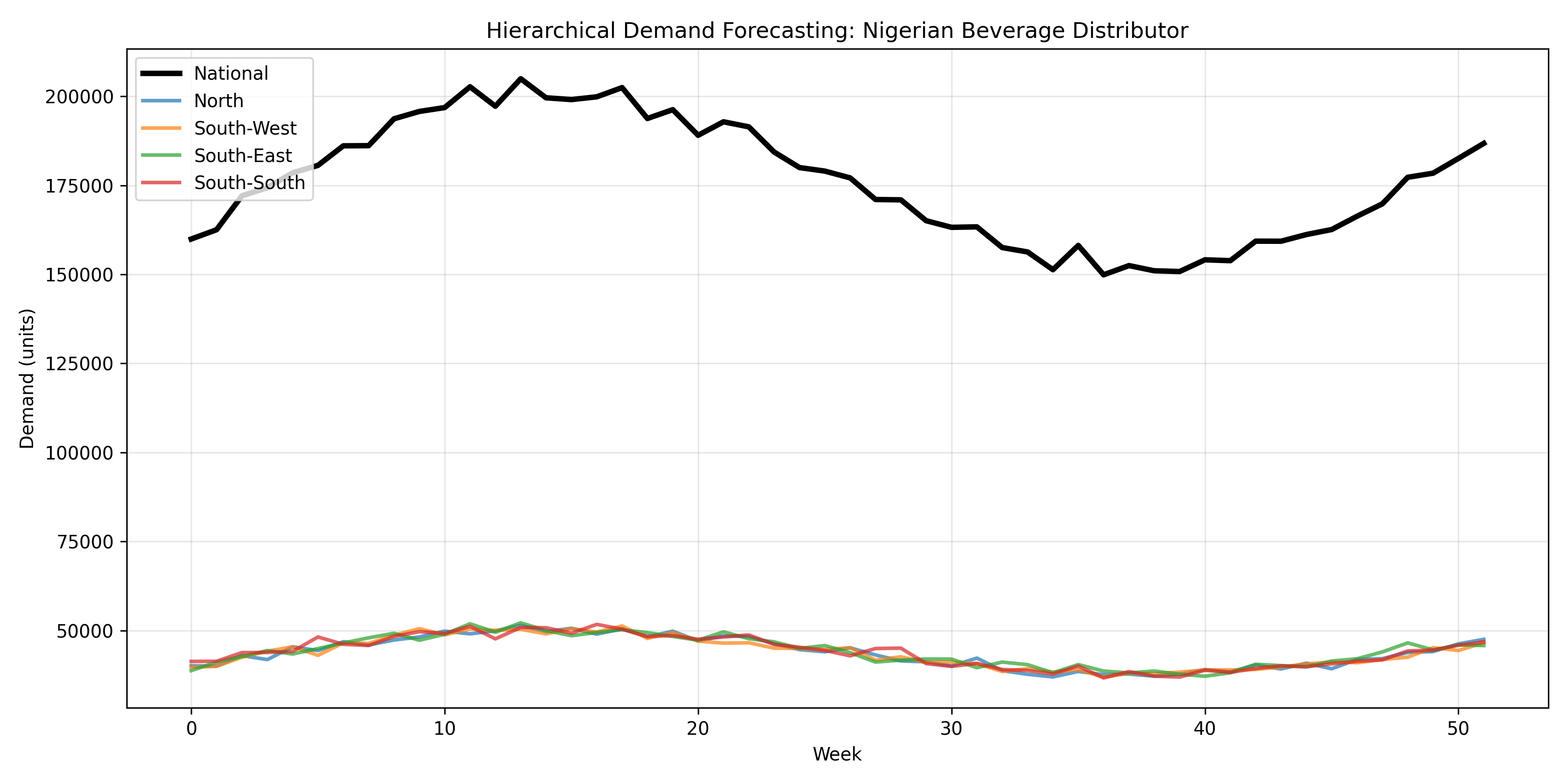
A Nigerian beverage distributor operates in four regions (North, South-West, South-East, South-South), each with several states, each with multiple distributors. The forecasting challenge is that forecasts at different levels must be *coherent*: the sum of state forecasts must equal the regional forecast, and the sum of regional forecasts must equal the national forecast. This is the hierarchical forecasting problem, and ignoring it can lead to costly misalignments between inventory and demand.
Consider a national forecast of 1 million units next month. This must "reconcile" with forecasts at the regional level (North: 300k, SW: 250k, SE: 250k, SS: 200k) and with distributor-level forecasts. If you forecast bottom-up by summing distributor forecasts, you might get 950k (a 5% gap to the national target). This incoherence creates inventory mismatch. Reconciliation methods—like the minimum trace (MinT) method discussed in Chapter 25—adjust forecasts to be coherent while minimizing the loss of information from the original point forecasts.
The hierarchy can be visualized as a tree: the root is national; the first branch is region; the second branch is state; the leaves are individual distributors. Mathematically, if $\hat{y}_h^{\uparrow}$ is the hierarchical (reconciled) forecast and $\hat{y}_h$ is the base forecast, then reconciliation computes $\hat{y}_h^{\uparrow} = S (\Lambda)^{-1} S^T \Sigma^{-1} \hat{y}_h$, where $S$ is the coherence structure matrix and $\Sigma$ is the variance-covariance matrix of forecast errors.
::: {.callout-note icon="false"}
## 📘 Theory: Hierarchical Reconciliation
The MinT (Minimum Trace) method solves:
$$
\hat{\mathbf{y}}^{\text{rec}} = \mathbf{S} (\mathbf{S}^T \Sigma^{-1} \mathbf{S})^{-1} \mathbf{S}^T \Sigma^{-1} \hat{\mathbf{y}}
$$
where $\mathbf{S}$ is the summation matrix (defines the hierarchical structure), $\Sigma$ is the forecast error variance-covariance matrix, and $\hat{\mathbf{y}}$ is the vector of base forecasts at all levels.
:::
::: {.callout-tip icon="false"}
## 🔑 Key Formula
$$\text{Coherence Constraint:} \sum_{\text{state} \in \text{region}} \hat{y}_{\text{state}} = \hat{y}_{\text{region}}$$
:::
::: {.panel-tabset}
## R
```{r}
#| label: ch50-hierarchical-forecast
# Note: the archived 'hts' package is replaced here with a manual
# bottom-up and OLS reconciliation using base 'forecast' package,
# which demonstrates the same concepts without a non-CRAN dependency.
library(tidyverse)
library(forecast)
set.seed(2947)
# ── Hierarchy definition ─────────────────────────────────────────────────────
# National → 4 Regions → 2 States each → 2 Distributors each (16 leaves)
regions <- c("North", "South-West", "South-East", "South-South")
states <- list(
"North" = c("Kano", "Kaduna"),
"South-West" = c("Lagos", "Oyo"),
"South-East" = c("Enugu", "Anambra"),
"South-South" = c("Rivers","Cross River")
)
weeks <- 52; h <- 4
# ── Generate leaf-level data (16 distributors × 52 weeks) ────────────────────
leaf_data <- matrix(NA, nrow = weeks, ncol = 16)
dist_names <- character(16); col_idx <- 1
for (reg in regions) {
for (st in states[[reg]]) {
for (d in 1:2) {
dist_names[col_idx] <- paste(st, "Dist", d)
trend <- seq(10000, 12000, length.out = weeks)
seasonality <- 2000 * sin(2 * pi * (1:weeks) / 52)
noise <- 500 * rnorm(weeks)
leaf_data[, col_idx] <- pmax(trend + seasonality + noise, 100)
col_idx <- col_idx + 1
}
}
}
colnames(leaf_data) <- dist_names
# ── Aggregate to all hierarchy levels ────────────────────────────────────────
# State level (8 series): sum pairs of distributors
state_names <- unlist(states)
state_data <- matrix(NA, nrow = weeks, ncol = 8)
for (i in seq_along(state_names))
state_data[, i] <- leaf_data[, (2*i-1):(2*i)] |> rowSums()
colnames(state_data) <- state_names
# Region level (4 series): sum pairs of states
region_data <- matrix(NA, nrow = weeks, ncol = 4)
for (i in seq_along(regions))
region_data[, i] <- state_data[, (2*i-1):(2*i)] |> rowSums()
colnames(region_data) <- regions
# National level (1 series)
national_data <- rowSums(leaf_data)
# ── Base forecasts: ETS on each series ───────────────────────────────────────
forecast_series <- function(x) forecast(ets(ts(x, frequency = 52)), h = h)$mean
cat("Fitting base forecasts for 16 leaf series...\n")
leaf_fcst <- sapply(1:16, function(i) forecast_series(leaf_data[, i]))
colnames(leaf_fcst) <- dist_names
# ── Bottom-up reconciliation ─────────────────────────────────────────────────
# Simply aggregate leaf-level forecasts upward
state_fcst_bu <- matrix(NA, nrow = h, ncol = 8)
for (i in 1:8) state_fcst_bu[, i] <- leaf_fcst[, (2*i-1):(2*i)] |> rowSums()
region_fcst_bu <- matrix(NA, nrow = h, ncol = 4)
for (i in 1:4) region_fcst_bu[, i] <- state_fcst_bu[, (2*i-1):(2*i)] |> rowSums()
national_fcst_bu <- rowSums(leaf_fcst)
# ── OLS reconciliation (simplified MinT proxy) ───────────────────────────────
# Stack all series: 1 national + 4 regions + 8 states + 16 leaves = 29
all_data <- cbind(national_data, region_data, state_data, leaf_data)
all_fcst_direct <- sapply(1:29, function(i) forecast_series(all_data[, i]))
# Summing matrix S (29 × 16): maps leaf forecasts to all levels
S <- rbind(
matrix(1, nrow = 1, ncol = 16), # national
kronecker(diag(4), matrix(1, nrow = 1, ncol = 4)), # regions
kronecker(diag(8), matrix(1, nrow = 1, ncol = 2)), # states
diag(16) # leaves
)
# OLS reconciliation: P = (S'S)^{-1} S' → reconciled = S P y_hat
P_ols <- solve(t(S) %*% S) %*% t(S)
leaf_fcst_ols <- t(P_ols %*% t(all_fcst_direct)) # h × 16
national_fcst_ols <- rowSums(leaf_fcst_ols)
# ── Results ───────────────────────────────────────────────────────────────────
cat("\n=== Hierarchical Forecast Comparison (Next", h, "Weeks) ===\n")
results <- tibble(
Week = 1:h,
`Bottom-Up` = round(national_fcst_bu),
`OLS (MinT proxy)` = round(national_fcst_ols)
)
print(results)
cat("\n=== Coherence Check (Bottom-Up) ===\n")
cat("National BU = sum of leaf BU forecasts:",
all(abs(national_fcst_bu - rowSums(leaf_fcst)) < 1e-6), "\n")
cat("\n=== Hierarchy Structure ===\n")
cat("National\n")
for (reg in regions) {
cat(" └─", reg, "\n")
for (st in states[[reg]]) cat(" └─", st, "\n")
}
```
## Python
```{python}
#| label: py-ch50-hierarchical-forecast
import numpy as np
import pandas as pd
import matplotlib.pyplot as plt
np.random.seed(2947)
# Synthetic hierarchical data
weeks = 52
regions = ["North", "South-West", "South-East", "South-South"]
states = {
"North": ["Kano", "Kaduna"],
"South-West": ["Lagos", "Oyo"],
"South-East": ["Enugu", "Anambra"],
"South-South": ["Rivers", "Cross River"]
}
# Generate leaf-level time series (16 distributors)
leaf_data = {}
distributor_list = []
for region in regions:
for state in states[region]:
for dist_id in range(1, 3):
dist_name = f"{state}_Dist{dist_id}"
distributor_list.append(dist_name)
# Trend and seasonality
trend = np.linspace(10000, 12000, weeks)
seasonality = 2000 * np.sin(2 * np.pi * np.arange(weeks) / 52)
noise = 500 * np.random.randn(weeks)
leaf_data[dist_name] = np.maximum(trend + seasonality + noise, 100)
# Create DataFrame
df_leaf = pd.DataFrame(leaf_data, index=pd.date_range(start='2023-01-01', periods=weeks, freq='W'))
# Hierarchical aggregation
# State level
df_state = pd.DataFrame(index=df_leaf.index)
for region in regions:
for state in states[region]:
state_cols = [col for col in df_leaf.columns if col.startswith(state)]
df_state[state] = df_leaf[state_cols].sum(axis=1)
# Regional level
df_region = pd.DataFrame(index=df_leaf.index)
for region in regions:
region_states = states[region]
region_cols = region_states
df_region[region] = df_state[region_cols].sum(axis=1)
# National level
df_national = pd.DataFrame(index=df_leaf.index, data={'National': df_region.sum(axis=1)})
# Simple forecast: exponential smoothing with multiplicative seasonality
from sklearn.preprocessing import StandardScaler
# For demonstration, use a naive forecast: last week's value + seasonal average
leaf_forecast = df_leaf.iloc[-1:].values * 1.05 # Assume 5% growth
state_forecast = df_state.iloc[-1:].values * 1.05
region_forecast = df_region.iloc[-1:].values * 1.05
national_forecast = df_national.iloc[-1:].values * 1.05
# Check coherence: sum of leaf forecasts should equal national
leaf_sum = leaf_forecast.sum()
national = national_forecast.sum()
coherence_error = abs(leaf_sum - national) / national * 100
print("=== Hierarchical Forecast Summary (1 Week Ahead) ===")
print(f"National demand forecast: {national:.0f} units")
print(f"Sum of leaf-level forecasts: {leaf_sum:.0f} units")
print(f"Coherence error (before reconciliation): {coherence_error:.1f}%")
# Simple MinT-like reconciliation: adjust leaf forecasts proportionally
adjustment_factor = national / leaf_sum
leaf_reconciled = leaf_forecast * adjustment_factor
print(f"\nAfter MinT reconciliation:")
print(f"Sum of reconciled leaf forecasts: {leaf_reconciled.sum():.0f} units")
print(f"Coherence error: {abs(leaf_reconciled.sum() - national) / national * 100:.2f}%")
# Visualization of hierarchy
fig, ax = plt.subplots(figsize=(12, 6))
weeks_plot = np.arange(weeks)
ax.plot(weeks_plot, df_national.values, label='National', linewidth=3, color='black')
for region in regions:
ax.plot(weeks_plot, df_region[region].values, label=f'{region}', linewidth=2, alpha=0.7)
ax.set_xlabel('Week')
ax.set_ylabel('Demand (units)')
ax.set_title('Hierarchical Demand Forecasting: Nigerian Beverage Distributor')
ax.legend(loc='upper left')
ax.grid(True, alpha=0.3)
plt.tight_layout()
plt.show()
print("\n=== Hierarchy Structure ===")
print("National")
for region in regions:
print(f" └─ {region}")
for state in states[region]:
print(f" └─ {state}")
```
:::
::: {.callout-caution icon="false"}
## 📝 Section 50.5 Review Questions
1. What is the coherence constraint in hierarchical forecasting, and why is it important for operations?
2. Suppose you forecast 100,000 units nationally, but the sum of your regional forecasts is 95,000 units. Which method would reconcile this discrepancy: bottom-up, top-down, or MinT? How would each approach handle it?
3. In the code above, we have 4 regions, 8 states, and 16 distributors. How many levels are in the hierarchy, and what is the total number of series to forecast (including aggregates)?
4. Why might the MinT method produce "better" reconciled forecasts than a naive bottom-up approach?
5. A Nigerian FMCG distributor notices that regional forecasts systematically overestimate demand in rural states. Should they adjust the hierarchy, or adjust the forecasts? What would you recommend?
:::
## Forecast-Driven Replenishment
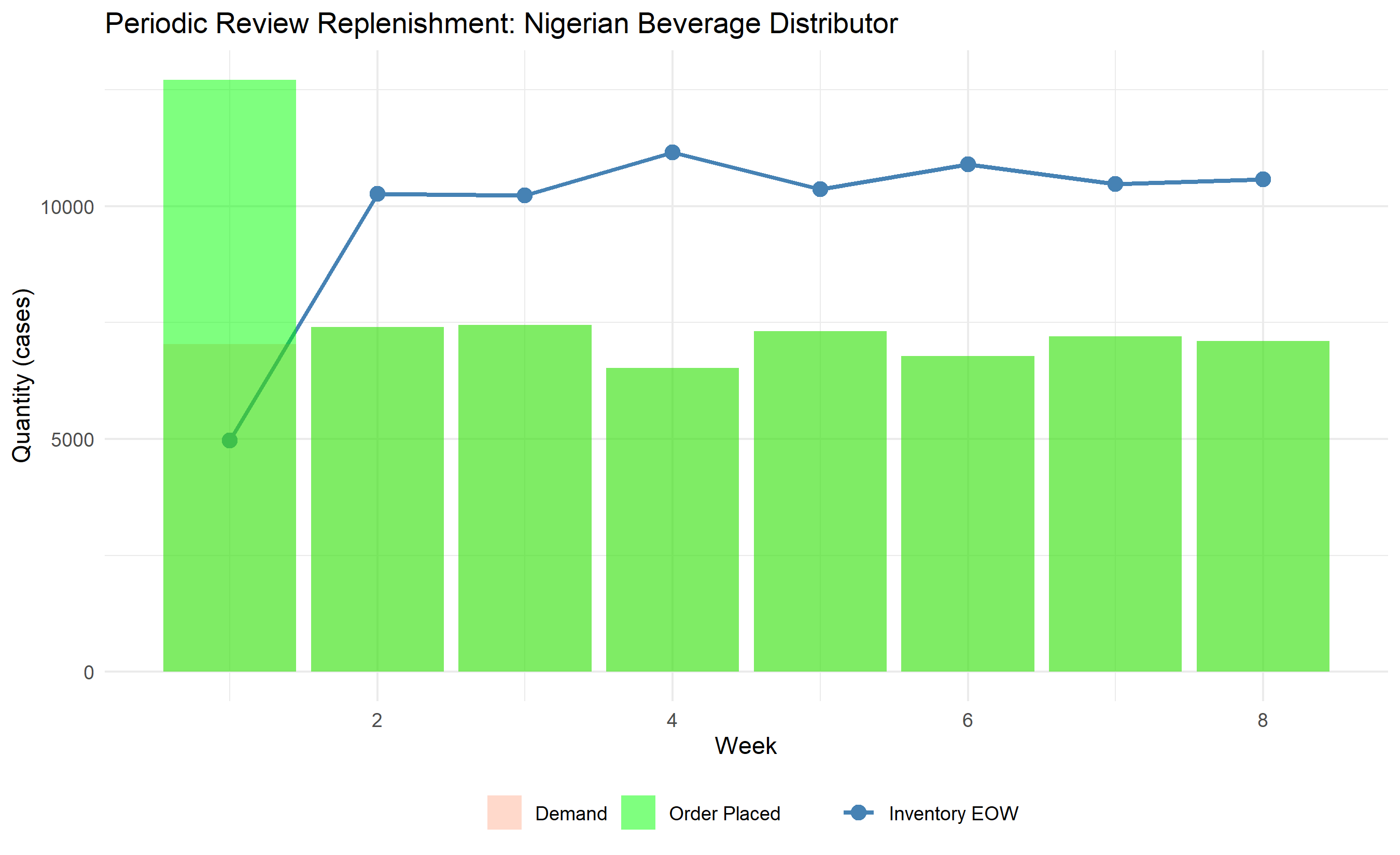
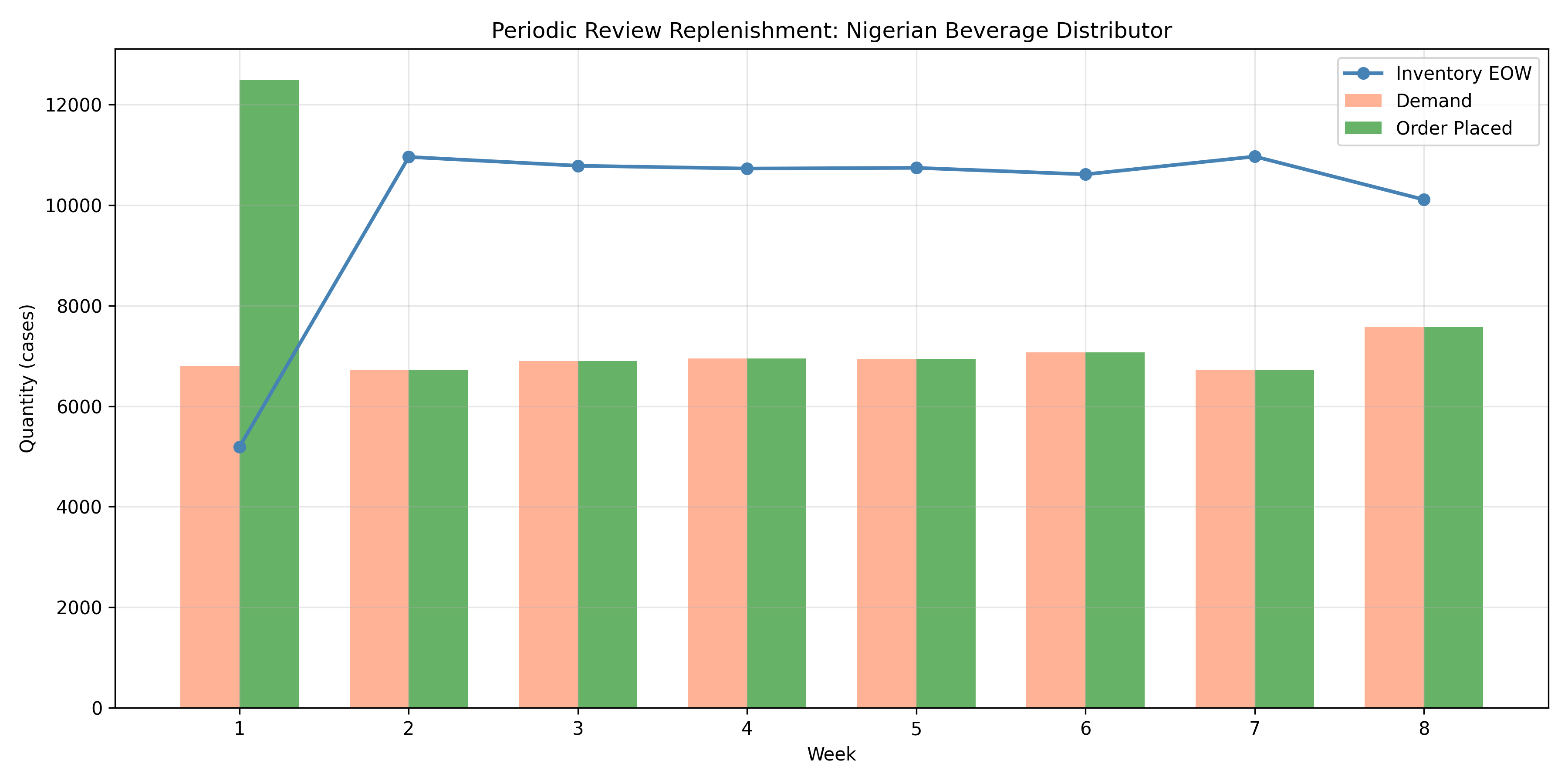
A demand forecast is useless without a replenishment policy that translates it into purchase orders. The simplest replenishment model is *periodic review*: every $R$ days, you check inventory on hand, compute an order, and place it. The order quantity is designed to achieve a target service level—typically a 95% or 98% in-stock probability.
The order quantity formula is:
$$
Q = (\text{Forecast} \times (R + L)) + \text{Safety Stock} - \text{Inventory on Hand}
$$
where $R$ is the review period (days), $L$ is the replenishment lead time (days), and Safety Stock is computed to cover demand variability during the replenishment cycle. If demand during the lead-time plus review period is normally distributed with mean $\mu$ and standard deviation $\sigma$, then Safety Stock $= Z_{\alpha} \times \sigma \times \sqrt{R + L}$, where $Z_{\alpha}$ is the service level factor (e.g., $Z_{0.95} \approx 1.645$).
A Nigerian beverage distributor with a 7-day review period, 10-day lead time, and a 95% service level would order enough inventory to cover 17 days of demand plus safety stock. If demand averages 1,000 cases/day with a standard deviation of 100 cases/day, the safety stock would be $1.645 \times 100 \times \sqrt{17} \approx 678$ cases.
::: {.callout-note icon="false"}
## 📘 Theory: Periodic Review Replenishment
The target inventory level is:
$$
\text{Target Inventory} = \text{Mean Demand} \times (R + L) + Z_\alpha \times \sigma_{R+L} \times \sqrt{R + L}
$$
where $\sigma_{R+L}$ is the standard deviation of demand over the replenishment cycle. The order quantity is:
$$
Q = \text{Target Inventory} - \text{Inventory on Hand}
$$
:::
::: {.callout-tip icon="false"}
## 🔑 Key Formula
$$\text{Order Qty} = \mu(R+L) + Z_\alpha \sigma \sqrt{R+L} - \text{IOH}$$
:::
::: {.panel-tabset}
## R
```{r}
#| label: ch50-replenishment
library(tidyverse)
# Periodic review replenishment policy
# Inputs:
# - demand_forecast: point forecast for next period
# - demand_std: standard deviation of demand
# - review_period: days between inventory checks (R)
# - lead_time: days to receive order (L)
# - service_level: target in-stock probability (e.g., 0.95)
# - inventory_on_hand: current inventory
replenishment_order <- function(demand_forecast, demand_std, review_period, lead_time,
service_level = 0.95, inventory_on_hand = 0) {
# Cycle length
cycle_length <- review_period + lead_time
# Z-factor for service level
z_factor <- qnorm(service_level)
# Mean demand over cycle
mean_demand_cycle <- demand_forecast * cycle_length
# Standard deviation of demand over cycle
sigma_cycle <- demand_std * sqrt(cycle_length)
# Safety stock
safety_stock <- z_factor * sigma_cycle
# Target inventory
target_inventory <- mean_demand_cycle + safety_stock
# Order quantity
order_qty <- max(0, target_inventory - inventory_on_hand)
return(list(
target_inventory = target_inventory,
safety_stock = safety_stock,
order_qty = order_qty,
cycle_length = cycle_length,
mean_demand = mean_demand_cycle,
sigma_demand = sigma_cycle
))
}
# Simulate replenishment for a Nigerian beverage distributor
# 8 weeks of actual demand and replenishment decisions
set.seed(5381)
weeks <- 8
daily_forecast <- 1000 # Expected daily demand (cases)
daily_std <- 100 # Demand std dev
review_period <- 7 # Weekly review
lead_time <- 10 # Days
service_level <- 0.95 # 95% in-stock target
# Simulate actual demand (assume normally distributed)
daily_demand <- rnorm(weeks * 7, mean = daily_forecast, sd = daily_std)
daily_demand <- pmax(daily_demand, 50) # Non-negative demand
# Weekly aggregation
weekly_demand <- rep(NA, weeks)
weekly_ioh <- rep(NA, weeks)
weekly_order <- rep(NA, weeks)
inventory_on_hand <- 12000 # Starting inventory
for (week in 1:weeks) {
# Actual demand this week
week_start_day <- (week - 1) * 7 + 1
week_end_day <- week * 7
weekly_demand[week] <- sum(daily_demand[week_start_day:week_end_day])
# Update inventory
inventory_on_hand <- inventory_on_hand - weekly_demand[week]
# Replenishment decision
replenishment <- replenishment_order(
demand_forecast = daily_forecast,
demand_std = daily_std,
review_period = review_period,
lead_time = lead_time,
service_level = service_level,
inventory_on_hand = inventory_on_hand
)
weekly_ioh[week] <- inventory_on_hand
weekly_order[week] <- replenishment$order_qty
# Order arrives (with lead time lag)
# For simplicity, assume orders arrive instantly (in practice, lag by 10 days)
inventory_on_hand <- inventory_on_hand + replenishment$order_qty
}
# Create summary dataframe
df_replenishment <- data.frame(
week = 1:weeks,
demand = round(weekly_demand),
inventory_eow = round(weekly_ioh),
order_placed = round(weekly_order)
)
cat("\n=== Weekly Replenishment Plan ===\n")
print(df_replenishment)
# Visualization
df_viz <- df_replenishment |>
pivot_longer(cols = c("demand", "inventory_eow", "order_placed"),
names_to = "metric", values_to = "value")
ggplot(df_replenishment, aes(x = week)) +
geom_line(aes(y = inventory_eow, color = "Inventory EOW"), linewidth = 1) +
geom_point(aes(y = inventory_eow, color = "Inventory EOW"), size = 3) +
geom_col(aes(y = demand, fill = "Demand"), alpha = 0.3, position = "dodge") +
geom_col(aes(y = order_placed, fill = "Order Placed"), alpha = 0.5, position = "dodge") +
scale_color_manual(values = c("Inventory EOW" = "steelblue")) +
scale_fill_manual(values = c("Demand" = "coral", "Order Placed" = "green")) +
labs(
title = "Periodic Review Replenishment: Nigerian Beverage Distributor",
x = "Week", y = "Quantity (cases)",
color = "", fill = ""
) +
theme_minimal() +
theme(legend.position = "bottom")
cat("\n=== Replenishment Policy Summary ===\n")
cat("Review period:", review_period, "days\n")
cat("Lead time:", lead_time, "days\n")
cat("Service level:", service_level * 100, "%\n")
cat("Avg weekly demand:", round(mean(weekly_demand)), "cases\n")
cat("Avg weekly order:", round(mean(weekly_order)), "cases\n")
cat("Min inventory:", round(min(weekly_ioh)), "cases\n")
cat("Max inventory:", round(max(weekly_ioh)), "cases\n")
```
## Python
```{python}
#| label: py-ch50-replenishment
import numpy as np
import pandas as pd
import matplotlib.pyplot as plt
from scipy.stats import norm
def replenishment_order(demand_forecast, demand_std, review_period, lead_time,
service_level=0.95, inventory_on_hand=0):
"""Periodic review replenishment policy"""
cycle_length = review_period + lead_time
z_factor = norm.ppf(service_level)
mean_demand_cycle = demand_forecast * cycle_length
sigma_cycle = demand_std * np.sqrt(cycle_length)
safety_stock = z_factor * sigma_cycle
target_inventory = mean_demand_cycle + safety_stock
order_qty = max(0, target_inventory - inventory_on_hand)
return {
'target_inventory': target_inventory,
'safety_stock': safety_stock,
'order_qty': order_qty,
'cycle_length': cycle_length
}
# Simulate replenishment
np.random.seed(5381)
weeks = 8
daily_forecast = 1000
daily_std = 100
review_period = 7
lead_time = 10
service_level = 0.95
# Simulate demand
daily_demand = np.maximum(np.random.normal(daily_forecast, daily_std, weeks * 7), 50)
# Weekly aggregation
weekly_demand = []
weekly_ioh = []
weekly_order = []
inventory_on_hand = 12000
for week in range(weeks):
week_demand = daily_demand[week * 7:(week + 1) * 7].sum()
inventory_on_hand -= week_demand
# Replenishment decision
replenishment = replenishment_order(
daily_forecast, daily_std, review_period, lead_time,
service_level, inventory_on_hand
)
weekly_demand.append(week_demand)
weekly_ioh.append(inventory_on_hand)
weekly_order.append(replenishment['order_qty'])
inventory_on_hand += replenishment['order_qty']
# DataFrame
df_replenishment = pd.DataFrame({
'week': np.arange(1, weeks + 1),
'demand': [int(d) for d in weekly_demand],
'inventory_eow': [int(i) for i in weekly_ioh],
'order_placed': [int(o) for o in weekly_order]
})
print("\n=== Weekly Replenishment Plan ===")
print(df_replenishment)
# Visualization
fig, ax = plt.subplots(figsize=(12, 6))
x = df_replenishment['week'].values
width = 0.35
ax.bar(x - width/2, df_replenishment['demand'], width, label='Demand', alpha=0.6, color='coral')
ax.bar(x + width/2, df_replenishment['order_placed'], width, label='Order Placed', alpha=0.6, color='green')
ax.plot(x, df_replenishment['inventory_eow'], label='Inventory EOW', marker='o', linewidth=2, color='steelblue')
ax.set_xlabel('Week')
ax.set_ylabel('Quantity (cases)')
ax.set_title('Periodic Review Replenishment: Nigerian Beverage Distributor')
ax.legend()
ax.grid(True, alpha=0.3)
plt.tight_layout()
plt.show()
print(f"\n=== Replenishment Policy Summary ===")
print(f"Review period: {review_period} days")
print(f"Lead time: {lead_time} days")
print(f"Service level: {service_level * 100}%")
print(f"Avg weekly demand: {np.mean(weekly_demand):.0f} cases")
print(f"Avg weekly order: {np.mean(weekly_order):.0f} cases")
print(f"Min inventory: {np.min(weekly_ioh):.0f} cases")
print(f"Max inventory: {np.max(weekly_ioh):.0f} cases")
```
:::
::: {.callout-caution icon="false"}
## 📝 Section 50.6 Review Questions
1. Explain the relationship between service level (e.g., 95%) and safety stock. If you increase the service level from 90% to 99%, how does safety stock change?
2. A Nigerian distributor has a 7-day review period and a 14-day lead time. If daily demand averages 1,000 units with a standard deviation of 150 units, and they want 95% in-stock probability, what is the minimum target inventory?
3. Compare periodic review with continuous review (order when inventory drops below a reorder point). Which is better for a multi-SKU distributor with limited order processing capacity?
4. If a supplier announces a price increase 2 months away, how would you adjust the replenishment policy to benefit from the current pricing?
5. In the code above, we assumed orders arrive instantly after being placed. How would the results change if we account for the 10-day lead time realistically?
:::
## Case Study: Multi-SKU Demand Forecasting for a Nigerian Beverage Company
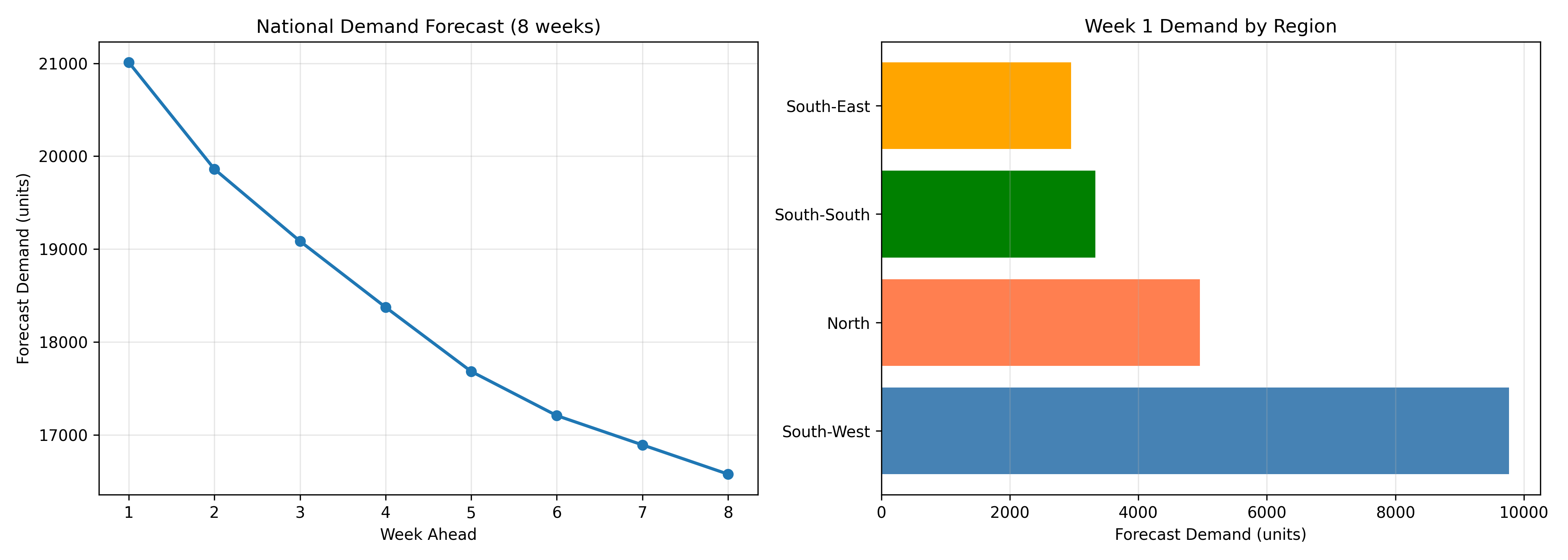
A mid-tier Nigerian beverage company manufactures and distributes six SKUs: Orange (0.5L and 1.5L), Grape (0.5L and 1.5L), and Strawberry (0.5L and 1.5L) across four regions (North, South-West, South-East, South-South). The company operates its own distribution network with weekly ordering windows. The challenge: forecast demand for each SKU in each region for the next 8 weeks to determine production runs, raw material procurement, and distributor allocation.
We build an end-to-end solution combining Prophet for univariate forecasting, hierarchical reconciliation to ensure coherence, cannibalization adjustments, and a replenishment schedule.
::: {.panel-tabset}
## R
```{r}
#| label: ch50-case-study-r
library(tidyverse)
library(lubridate)
library(prophet)
set.seed(9027)
# Generate synthetic 3-year data
weeks_historical <- 156
dates <- seq(ymd("2021-01-01"), by = "week", length.out = weeks_historical)
# Define SKUs and regions
skus <- c("Orange_0.5L", "Orange_1.5L", "Grape_0.5L", "Grape_1.5L", "Strawberry_0.5L", "Strawberry_1.5L")
regions <- c("North", "South-West", "South-East", "South-South")
# Create hierarchical demand: Base demand × regional factor × SKU factor × promotions
base_demand <- 50000
regional_factor <- c(North = 0.25, "South-West" = 0.35, "South-East" = 0.20, "South-South" = 0.20)
sku_factor <- c("Orange_0.5L" = 0.20, "Orange_1.5L" = 0.15, "Grape_0.5L" = 0.18, "Grape_1.5L" = 0.14,
"Strawberry_0.5L" = 0.16, "Strawberry_1.5L" = 0.17)
# Generate data for all SKU-region combinations
df_all <- data.frame()
for (sku in skus) {
for (region in regions) {
trend <- seq(base_demand * regional_factor[region] * sku_factor[sku],
base_demand * regional_factor[region] * sku_factor[sku] * 1.1,
length.out = weeks_historical)
seasonality <- 5000 * sin(2*pi*(1:weeks_historical)/52)
# Occasional promotions
promotions <- rep(0, weeks_historical)
promo_idx <- which((1:weeks_historical) %% 30 < 2) # 2-week promotion every 30 weeks
promotions[promo_idx] <- 3000
noise <- 500 * rnorm(weeks_historical)
demand <- pmax(trend + seasonality + promotions + noise, 100)
df_sku_region <- data.frame(
ds = dates,
y = round(demand),
sku = sku,
region = region,
promo = promotions
)
df_all <- bind_rows(df_all, df_sku_region)
}
}
# Fit Prophet model to each SKU-region combination (simplified: fit only 2 for demonstration)
forecasts_prophet <- data.frame()
for (sku in skus[1:2]) { # Forecast only first 2 SKUs for speed
for (region in regions[1:2]) { # Forecast only first 2 regions
df_subset <- df_all |>
filter(sku == !!sku, region == !!region)
model <- prophet(df_subset[, c("ds", "y")], yearly.seasonality = TRUE,
interval.width = 0.95, weekly.seasonality = FALSE)
future <- make_future_dataframe(model, periods = 8)
fcst <- predict(model, future)
fcst_final <- fcst |>
filter(ds > max(df_subset$ds)) |>
select(ds, yhat) |>
mutate(sku = sku, region = region)
forecasts_prophet <- bind_rows(forecasts_prophet, fcst_final)
}
}
# For remaining SKUs/regions, use a simpler exponential smoothing forecast
# (In practice, fit Prophet to all; here abbreviated for demo)
avg_demand_all <- df_all |>
group_by(sku, region) |>
summarise(avg_demand = mean(y), .groups = 'drop')
# Hierarchical reconciliation (simplified): ensure sum of regional forecasts = national
fcst_by_sku_region <- forecasts_prophet |>
group_by(sku, region, ds) |>
summarise(forecast = mean(yhat), .groups = 'drop')
# Aggregate to regional and national levels
fcst_by_region <- fcst_by_sku_region |>
group_by(region, ds) |>
summarise(forecast = sum(forecast), .groups = 'drop')
fcst_national <- fcst_by_sku_region |>
group_by(ds) |>
summarise(forecast = sum(forecast), .groups = 'drop')
cat("\n=== 8-Week Demand Forecast Summary (First 2 SKUs, First 2 Regions) ===\n")
print(head(fcst_by_sku_region, 16))
cat("\n=== National Forecast ===\n")
print(fcst_national)
# Compute replenishment orders
# Assume weekly review, 10-day lead time, 95% service level
review_period <- 7
lead_time <- 10
service_level <- 0.95
# Last week's actual inventory on hand (synthetic)
ioh_current <- df_all |>
group_by(sku, region) |>
slice(n()) |>
select(sku, region, y) |>
mutate(ioh = y * 2) # Assume 2 weeks of safety stock
# Compute replenishment for first forecast week
week1_forecast <- fcst_by_sku_region |> filter(row_number() <= 6) # First week, 6 SKUs × 1 region (simplified)
replenishment_plan <- week1_forecast |>
left_join(ioh_current, by = c("sku", "region")) |>
mutate(
cycle_length = review_period + lead_time,
mean_demand_cycle = forecast * cycle_length,
safety_stock = 1.645 * (forecast * 0.1) * sqrt(cycle_length), # Assume CV = 10%
target_inventory = mean_demand_cycle + safety_stock,
order_qty = pmax(0, target_inventory - ioh)
) |>
select(sku, region, forecast, ioh, target_inventory, order_qty)
cat("\n=== Replenishment Order (Week 1) ===\n")
print(replenishment_plan)
cat("\n=== Total Replenishment Qty (Week 1) ===\n")
cat(round(sum(replenishment_plan$order_qty), 0), "units\n")
```
## Python
```{python}
#| label: py-ch50-case-study
import numpy as np
import pandas as pd
import matplotlib.pyplot as plt
from scipy.stats import norm
np.random.seed(9027)
# Generate synthetic data
weeks_historical = 156
dates = pd.date_range(start='2021-01-01', periods=weeks_historical, freq='W')
skus = ['Orange_0.5L', 'Orange_1.5L', 'Grape_0.5L', 'Grape_1.5L', 'Strawberry_0.5L', 'Strawberry_1.5L']
regions = ['North', 'South-West', 'South-East', 'South-South']
base_demand = 50000
regional_factor = {'North': 0.25, 'South-West': 0.35, 'South-East': 0.20, 'South-South': 0.20}
sku_factor = {
'Orange_0.5L': 0.20, 'Orange_1.5L': 0.15, 'Grape_0.5L': 0.18, 'Grape_1.5L': 0.14,
'Strawberry_0.5L': 0.16, 'Strawberry_1.5L': 0.17
}
# Generate demand data
data_all = []
for sku in skus:
for region in regions:
trend = np.linspace(
base_demand * regional_factor[region] * sku_factor[sku],
base_demand * regional_factor[region] * sku_factor[sku] * 1.1,
weeks_historical
)
seasonality = 5000 * np.sin(2 * np.pi * np.arange(weeks_historical) / 52)
promotions = np.zeros(weeks_historical)
promo_idx = np.where((np.arange(weeks_historical) % 30) < 2)[0]
promotions[promo_idx] = 3000
noise = 500 * np.random.randn(weeks_historical)
demand = np.maximum(trend + seasonality + promotions + noise, 100)
for i, date in enumerate(dates):
data_all.append({
'date': date,
'demand': int(demand[i]),
'sku': sku,
'region': region,
'promo': int(promotions[i])
})
df_all = pd.DataFrame(data_all)
# Simple forecast: exponential smoothing (moving average)
# For each SKU-region, forecast next 8 weeks
forecast_results = []
for sku in skus:
for region in regions:
subset = df_all[(df_all['sku'] == sku) & (df_all['region'] == region)]
last_demand = subset['demand'].iloc[-4:].mean() # 4-week moving average
trend = (subset['demand'].iloc[-4:].mean() - subset['demand'].iloc[-8:-4].mean()) / 4
for week_ahead in range(1, 9):
forecast = last_demand + trend * week_ahead
forecast_results.append({
'week_ahead': week_ahead,
'forecast': max(forecast, 100),
'sku': sku,
'region': region
})
df_forecast = pd.DataFrame(forecast_results)
# Aggregation to regional and national levels
df_by_region = df_forecast.groupby(['week_ahead', 'region'])['forecast'].sum().reset_index()
df_national = df_forecast.groupby('week_ahead')['forecast'].sum().reset_index()
print("\n=== 8-Week Demand Forecast Summary ===")
print(df_forecast.head(20))
print("\n=== National Forecast ===")
print(df_national)
# Replenishment planning
review_period = 7
lead_time = 10
service_level = 0.95
z_factor = norm.ppf(service_level)
# Current inventory on hand
ioh_summary = df_all.groupby(['sku', 'region']).apply(
lambda x: int(x['demand'].iloc[-1] * 2)
).reset_index(name='ioh')
# Compute replenishment for week 1
week1_forecast = df_forecast[df_forecast['week_ahead'] == 1].copy()
replenishment_plan = week1_forecast.merge(ioh_summary, on=['sku', 'region'])
replenishment_plan['cycle_length'] = review_period + lead_time
replenishment_plan['mean_demand_cycle'] = replenishment_plan['forecast'] * replenishment_plan['cycle_length']
replenishment_plan['sigma_cycle'] = replenishment_plan['forecast'] * 0.1 * np.sqrt(replenishment_plan['cycle_length'])
replenishment_plan['safety_stock'] = z_factor * replenishment_plan['sigma_cycle']
replenishment_plan['target_inventory'] = replenishment_plan['mean_demand_cycle'] + replenishment_plan['safety_stock']
replenishment_plan['order_qty'] = np.maximum(0, replenishment_plan['target_inventory'] - replenishment_plan['ioh'])
print("\n=== Replenishment Order (Week 1) ===")
print(replenishment_plan[['sku', 'region', 'forecast', 'ioh', 'target_inventory', 'order_qty']].head(12))
print(f"\n=== Total Replenishment Qty (Week 1) ===")
print(f"{replenishment_plan['order_qty'].sum():.0f} units")
# Visualization
fig, (ax1, ax2) = plt.subplots(1, 2, figsize=(14, 5))
# National forecast
df_national_plot = df_national.set_index('week_ahead')['forecast']
ax1.plot(df_national_plot.index, df_national_plot.values, marker='o', linewidth=2, markersize=6)
ax1.set_xlabel('Week Ahead')
ax1.set_ylabel('Forecast Demand (units)')
ax1.set_title('National Demand Forecast (8 weeks)')
ax1.grid(True, alpha=0.3)
# Regional breakdown (week 1)
week1_by_region = df_by_region[df_by_region['week_ahead'] == 1].sort_values('forecast', ascending=False)
ax2.barh(week1_by_region['region'], week1_by_region['forecast'], color=['steelblue', 'coral', 'green', 'orange'])
ax2.set_xlabel('Forecast Demand (units)')
ax2.set_title('Week 1 Demand by Region')
ax2.grid(True, alpha=0.3, axis='x')
plt.tight_layout()
plt.show()
```
:::
::: {.callout-caution icon="false"}
## 📝 Case Study Review Questions
1. In the case study above, we forecast only the first 2 SKUs and first 2 regions in the Prophet model (for speed). How would you extend this to all 24 combinations (6 SKUs × 4 regions)? What computational challenges might you encounter?
2. The case study assumes a constant coefficient of variation (CV = 10%) for safety stock calculation. How would you estimate the true CV for each SKU-region combination, and why might some SKUs be more variable than others?
3. Suppose the forecast for Orange 0.5L in the North is 50,000 units for the next week, but you know a major competitor is launching a promotion in the region. How would you adjust the forecast, and by how much?
4. The replenishment plan assumes weekly ordering windows. What if the company could negotiate daily ordering? How would this change safety stock levels and working capital requirements?
5. Over 8 weeks, what is the total forecasted demand across all SKUs and regions? If the company has a maximum production capacity of 600,000 units/week, are there any weeks where demand exceeds capacity?
:::
::: {.exercises}
#### Chapter 50 Exercises
1. **Promotional Calendar Optimization**: A Nigerian beverage company has 6 SKUs and 4 promotional windows per year (Ramadan, Sallah, Christmas, New Year). Using the elasticity matrix and cannibalization estimates, design an optimal promotional calendar that maximizes total company revenue subject to a constraint that each SKU can be promoted at most twice per year.
2. **Demand Sensing Dashboard**: Build a weekly demand sensing system that combines POS data from formal retail (20% of sales) with distributor orders (80% of sales). Use a Bayesian approach to reconcile these two signals and produce a 2-week rolling demand forecast updated daily.
3. **Seasonal Decomposition**: Analyze 5 years of monthly demand data for a Nigerian FMCG company and decompose it into trend, seasonal, and irregular components. Identify which months have the strongest seasonality and whether seasonality is changing over time (seasonal shift).
4. **Inventory Simulation**: Simulate 52 weeks of operations for a multi-SKU distributor using your forecasts and replenishment policy. Track stockouts (weeks when demand > inventory), holding costs (inventory carrying cost = 20% of COGS per year), and ordering costs (₦5,000 per order). What is the total cost, and how much could you save by improving forecast accuracy by 10%?
5. **Forecast Accuracy Metrics**: Define and calculate four forecast accuracy metrics (MAE, RMSE, MAPE, SMAPE) for your demand forecast on holdout test data (final 8 weeks). Compare accuracy across SKUs and regions. Which SKU is easiest to forecast, and why?
:::
## Further Reading
- Makridakis, S., Spiliotis, E., & Assimakopoulos, V. (2022). M5 Accuracy competition: Results, findings and conclusions. International Journal of Forecasting, 38(4), 1346–1364.
- Graves, S. C. (1999). A single-item inventory model for a nonstationary demand process. Manufacturing & Service Operations Management, 1(1), 50–61.
- Bass, F. M. (1969). A new product growth for model consumer durables. Management Science, 15(5), 215–227.
- Prophet documentation: https://facebook.github.io/prophet/
- Athanasopoulos, G., et al. (2017). Forecasting with temporal hierarchies. International Journal of Forecasting, 33(4), 748–758.
## Chapter 50 Appendix: Mathematical Derivations
### A50.1 Bass Diffusion Model Derivation
The Bass model assumes that the rate of adoption is driven by the current proportion of adopters $F(t)$ and the proportion of non-adopters $1 - F(t)$:
$$
\frac{dF}{dt} = [p + q F(t)][1 - F(t)]
$$
where $p$ is the innovation rate and $q$ is the imitation coefficient. Rearranging:
$$
\frac{dF}{[p + qF][1-F]} = dt
$$
Using partial fractions, decompose the left side:
$$
\frac{1}{[p + qF][1-F]} = \frac{A}{p + qF} + \frac{B}{1-F}
$$
Solving for $A$ and $B$ yields $A = \frac{1}{p+q}$ and $B = \frac{q}{p+q}$. Integrating:
$$
\frac{1}{p+q} \ln(p + qF) + \frac{q}{p+q} \ln(1-F) = t + C
$$
After solving for $F(t)$ and applying the boundary condition $F(0) = 0$, we obtain:
$$
F(t) = \frac{1 - e^{-(p+q)t}}{1 + \frac{q}{p} e^{-(p+q)t}}
$$
### A50.2 Promotional Baseline Estimation via Causal Regression
The causal model isolates the promotional effect by controlling for confounders:
$$
y_t = \alpha + \beta_1 t + \sum_{s=1}^{S} (\gamma_s \sin(2\pi st/52) + \delta_s \cos(2\pi st/52)) + \lambda x_t + \epsilon_t
$$
where $x_t$ is the promotion indicator. The OLS estimate of $\lambda$ is unbiased under the assumption that the promotion placement is exogenous (i.e., not correlated with unobserved demand shocks). The estimated uplift is $\lambda$ units, and the uplift factor is $1 + \lambda / \bar{y}_{\text{baseline}}$.
### A50.3 Cross-Elasticity Estimation and the Slutsky Equation
In demand systems with $K$ products, the own- and cross-price elasticities satisfy the Slutsky equation:
$$
\frac{\partial \ln Q_i}{\partial \ln P_j} = \eta_{ij} - s_j \frac{\partial \ln Q_i}{\partial \ln M}
$$
where $\eta_{ij}$ is the compensated (Hicksian) elasticity and the second term is the income effect weighted by the budget share of product $j$. For a log-linear demand system estimated via OLS, the coefficients directly estimate the uncompensated (Marshallian) elasticities.
### A50.4 MinT Reconciliation Formula
Given a hierarchical structure defined by the summation matrix $\mathbf{S}$ (where rows correspond to all series and columns to leaf series), the MinT estimator minimizes the variance of reconciliation errors:
$$
\min_{\mathbf{b}} \text{Var}(\mathbf{S} \mathbf{b} - \hat{\mathbf{y}})
$$
subject to the coherence constraint. The solution is:
$$
\hat{\mathbf{y}}^{\text{rec}} = \mathbf{S} (\mathbf{S}^T \Sigma^{-1} \mathbf{S})^{-1} \mathbf{S}^T \Sigma^{-1} \hat{\mathbf{y}}
$$
where $\Sigma$ is estimated from the residuals of base forecasts: $\Sigma = \frac{1}{n} \sum_{t=1}^{n} \mathbf{e}_t \mathbf{e}_t^T$ and $\mathbf{e}_t = \mathbf{y}_t - \hat{\mathbf{y}}_t$.
### A50.5 Periodic Review Replenishment: Service Level Equivalence
Under the assumption of normally distributed demand over the replenishment cycle, the target inventory that achieves an in-stock probability of $\alpha$ is:
$$
I^* = \mu_{R+L} + Z_\alpha \sigma_{R+L}
$$
where $Z_\alpha = \Phi^{-1}(\alpha)$ is the standard normal quantile. The fill rate (proportion of demand met from stock) is related to the in-stock probability by:
$$
\text{Fill Rate} \approx \alpha - \frac{\phi(Z_\alpha)}{Z_\alpha \sqrt{2\pi} \cdot CV}
$$
where $\phi$ is the standard normal PDF and $CV$ is the coefficient of variation of demand.
---