---
title: "Regression for Business: Predictive Sales Analytics"
---
```{python}
#| label: python-setup-11-predictive-sales
#| include: false
import numpy as np
import pandas as pd
import matplotlib.pyplot as plt
import seaborn as sns
from datetime import datetime, timedelta
from sklearn.linear_model import LinearRegression, Ridge, Lasso, RidgeCV, LassoCV
from sklearn.metrics import mean_squared_error, mean_absolute_error
```
::: {.callout-note icon="false"}
## 📋 Learning Objectives
By the end of this chapter, you will be able to:
- Design and implement sales forecasting models aligned with business objectives
- Engineer time-based, lag, and rolling average features from transactional data
- Build a complete sales prediction pipeline from raw data to deployment
- Identify and use leading indicators for forward-looking forecasts
- Communicate model results and confidence intervals to non-technical stakeholders
- Create actionable dashboards that drive sales management decisions
- Handle real-world complications: seasonality, promotions, outliers, structural breaks
:::
## Sales Analytics: The Business Context
Sales forecasting is one of the highest-ROI applications of analytics. Accurate predictions enable:
- **Inventory optimisation:** Stock right amount of product; reduce stockouts and overstock
- **Revenue planning:** Set realistic budgets and targets; motivate teams
- **Promotional planning:** When and where to run promotions; measure incremental impact
- **Capacity planning:** Hire, allocate resources, manage supply chain
- **Cash flow forecasting:** Plan working capital, debt service
### Types of Sales Prediction Problems
| Problem | Horizon | Granularity | Drivers | Example |
|---|---|---|---|---|
| **Demand forecasting** | 1–24 months | Product × Location | Historical seasonality, trends, promotions | Forecast Q2 demand for SKU "Flour" in Lagos |
| **Lead scoring** | Deal-by-deal | Opportunity | Prospect profile, engagement | Predict probability a sales lead closes |
| **Customer churn** | 3–12 months | Customer | Engagement, spending, support tickets | Predict high-value customer attrition |
| **Upsell prediction** | 1–3 months | Customer × Product | Purchase history, firmographics | Predict customer receptiveness to premium tier |
### Forecast vs Prediction
- **Forecast:** Extrapolate time series forward (often univariate, assumes past patterns continue)
- **Prediction:** Model outcome given explanatory variables (multivariate, causal reasoning)
Regression-based sales models are **predictive**, using leading indicators to anticipate outcomes.
::: {.callout-caution icon="false"}
## 📝 Section 11.1 Review Questions
1. Why is accurate sales forecasting valuable to a business?
2. Distinguish forecast from prediction. When would you use each?
3. List three leading indicators for FMCG product demand.
4. What is the difference between demand forecasting and lead scoring?
:::
## Feature Engineering for Sales
Raw sales data (transactions, timestamps, product codes) must be transformed into predictive features.
::: {.callout-note icon="false"}
## 📘 Theory: Feature Engineering Categories
1. **Time-based features:**
- Month, quarter, year
- Day of week, day of month, day of year
- Holiday flags (national, regional, religious)
- Seasonal indicators (rainy season, year-end, post-harvest)
2. **Lag features:**
- Sales last week (s_t−1), last month, last year (s_t−12)
- Capture temporal dependencies and trend persistence
- Useful for time-series data where recent history predicts near future
3. **Rolling aggregates:**
- 7-day, 30-day rolling average (smooths volatility)
- Rolling standard deviation (captures seasonality/variability)
- Useful for detrending and trend extraction
4. **Categorical/promotional:**
- Indicator for running promotion (binary or intensity)
- Competitor pricing or availability
- Sales force activity (calls, site visits)
- External shocks (supply disruption, competitor launch)
5. **Macro indicators:**
- Inflation, exchange rates (for import-dependent goods)
- Unemployment, GDP growth (proxy for consumer spending)
- Fuel prices (affects logistics costs and demand for transport/energy products)
:::
### Worked Example: FMCG Feature Engineering
::: {.panel-tabset}
## R
```{r}
library(tidyverse)
library(lubridate)
library(zoo)
# Simulate Nigerian FMCG data: daily sales of 5 SKUs across 3 regions (2019-2023, 5 years = 1,825 days)
set.seed(42)
dates <- seq(from = as.Date("2019-01-01"), to = as.Date("2023-12-31"), by = "day")
n_days <- length(dates)
products <- c("Flour", "Sugar", "Oil", "Rice", "Salt")
regions <- c("Lagos", "Abuja", "Kano")
# Create grid of all combinations
data_raw <- expand_grid(
date = dates,
product = products,
region = regions
)
# Add sales (with seasonality and trends)
data_raw <- data_raw |>
mutate(
day_of_year = yday(date),
month = month(date),
year = year(date),
day_of_week = wday(date),
# Base sales by product
base_sales = case_when(
product == "Flour" ~ 5000,
product == "Sugar" ~ 3500,
product == "Oil" ~ 4000,
product == "Rice" ~ 6000,
product == "Salt" ~ 2000
),
# Regional multiplier
region_mult = case_when(
region == "Lagos" ~ 1.5,
region == "Abuja" ~ 1.0,
region == "Kano" ~ 0.8
),
# Seasonality (rainy season boost for some products)
seasonal_boost = 1 + 0.3 * sin(2 * pi * day_of_year / 365),
# Trend (growing market)
trend = 1 + 0.05 * (year - 2019),
# Weekend boost for retail
weekend_boost = 1 + 0.1 * (day_of_week %in% c(1, 7)),
# Promotion (once per month, 20% boost)
is_promo = (day(date) <= 7) & (day_of_week == 5),
promo_boost = 1 + 0.2 * is_promo,
# Noise
noise = rnorm(n(), mean = 1, sd = 0.1),
# Final sales
sales = base_sales * region_mult * seasonal_boost * trend * weekend_boost * promo_boost * noise,
sales = pmax(sales, 0) # Floor at zero
) |>
select(date, product, region, sales, month, year, day_of_week, is_promo)
cat("Raw FMCG Data:\n")
print(head(data_raw, 10))
# Feature Engineering
data_features <- data_raw |>
arrange(product, region, date) |>
group_by(product, region) |>
mutate(
# Lags
sales_lag1 = lag(sales, 1), # Last day
sales_lag7 = lag(sales, 7), # Same weekday last week
sales_lag30 = lag(sales, 30), # Last month
sales_lag365 = lag(sales, 365), # Same day last year
# Rolling averages
sales_ma7 = rollmean(sales, k = 7, fill = NA, align = "right"),
sales_ma30 = rollmean(sales, k = 30, fill = NA, align = "right"),
# Trend: rolling standard deviation (volatility)
sales_sd7 = rollapply(sales, width = 7, FUN = sd, fill = NA, align = "right"),
# Year-on-year growth
yoy_growth = (sales - sales_lag365) / (sales_lag365 + 1),
# Time features
month = month(date),
quarter = quarter(date),
day_of_month = day(date),
is_weekend = wday(date) %in% c(1, 7),
is_month_start = day(date) <= 7,
is_month_end = day(date) >= 24
) |>
ungroup()
cat("\n\nFeatures after engineering:\n")
print(head(data_features |> select(date, product, region, sales, sales_lag1, sales_lag7,
sales_ma7, sales_ma30, month, is_weekend, is_promo), 10))
# Summary of features
cat("\n\nFeature Summary:\n")
cat("Lag features: sales_lag1, sales_lag7, sales_lag30, sales_lag365\n")
cat("Rolling aggregates: sales_ma7, sales_ma30, sales_sd7\n")
cat("Time features: month, quarter, day_of_month, is_weekend, is_month_start, is_month_end\n")
cat("Promotional: is_promo\n")
cat("Transformations: yoy_growth\n")
# Visualise key patterns
par(mfrow = c(2, 2), mar = c(5, 5, 3, 1))
# Plot 1: Sales over time for one product
flour_data <- data_features |> filter(product == "Flour", region == "Lagos") |> arrange(date)
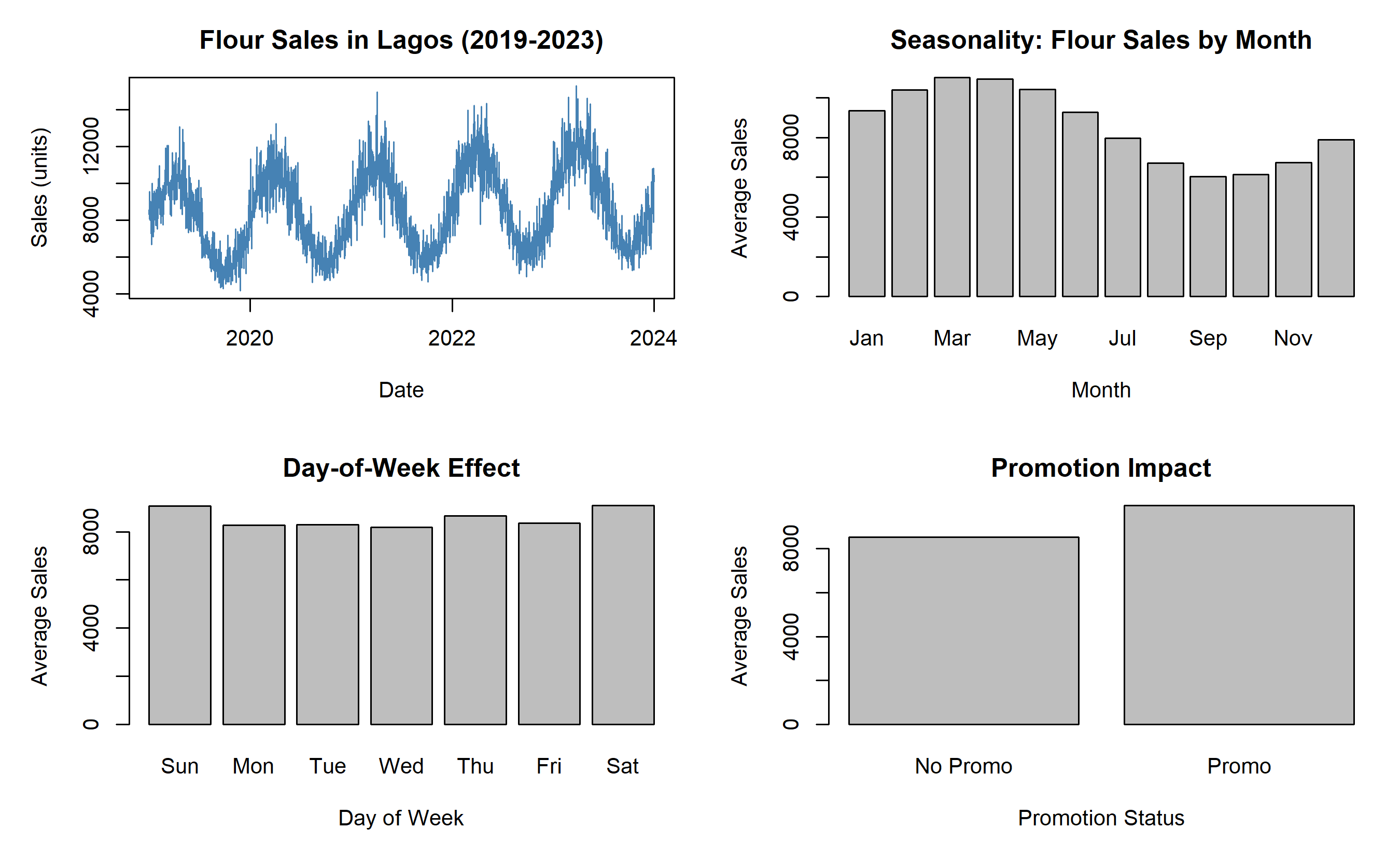
plot(flour_data$date, flour_data$sales, type = "l", lwd = 1, col = "steelblue",
xlab = "Date", ylab = "Sales (units)", main = "Flour Sales in Lagos (2019-2023)")
# Plot 2: Seasonal pattern
flour_by_month <- data_features |> filter(product == "Flour", region == "Lagos") |>
group_by(month) |> summarise(avg_sales = mean(sales, na.rm = TRUE))
barplot(flour_by_month$avg_sales, names.arg = month.abb, xlab = "Month",
ylab = "Average Sales", main = "Seasonality: Flour Sales by Month")
# Plot 3: Day-of-week effect
flour_by_dow <- data_features |> filter(product == "Flour", region == "Lagos") |>
group_by(day_of_week) |> summarise(avg_sales = mean(sales, na.rm = TRUE))
barplot(flour_by_dow$avg_sales, names.arg = c("Sun", "Mon", "Tue", "Wed", "Thu", "Fri", "Sat"),
xlab = "Day of Week", ylab = "Average Sales", main = "Day-of-Week Effect")
# Plot 4: Promotion impact
flour_promo_vs_no <- data_features |> filter(product == "Flour", region == "Lagos") |>
group_by(is_promo) |> summarise(avg_sales = mean(sales, na.rm = TRUE))
barplot(flour_promo_vs_no$avg_sales, names.arg = c("No Promo", "Promo"),
xlab = "Promotion Status", ylab = "Average Sales", main = "Promotion Impact")
par(mfrow = c(1, 1))
```
## Python
```{python}
import pandas as pd
import numpy as np
import matplotlib.pyplot as plt
from datetime import timedelta
np.random.seed(42)
# Generate date range
dates = pd.date_range(start='2019-01-01', end='2023-12-31', freq='D')
products = ['Flour', 'Sugar', 'Oil', 'Rice', 'Salt']
regions = ['Lagos', 'Abuja', 'Kano']
# Create grid
data_raw = []
for date in dates:
for product in products:
for region in regions:
day_of_year = date.dayofyear
month = date.month
year = date.year
day_of_week = date.weekday()
# Base sales
base_sales = {'Flour': 5000, 'Sugar': 3500, 'Oil': 4000, 'Rice': 6000, 'Salt': 2000}[product]
region_mult = {'Lagos': 1.5, 'Abuja': 1.0, 'Kano': 0.8}[region]
# Seasonality
seasonal_boost = 1 + 0.3 * np.sin(2 * np.pi * day_of_year / 365)
trend = 1 + 0.05 * (year - 2019)
weekend_boost = 1 + 0.1 * (day_of_week in [5, 6]) # Fri, Sat
# Promotion
is_promo = (date.day <= 7) and (day_of_week == 4) # Thursday
promo_boost = 1 + 0.2 * is_promo
# Noise
noise = np.random.normal(1, 0.1)
# Final sales
sales = max(0, base_sales * region_mult * seasonal_boost * trend * weekend_boost * promo_boost * noise)
data_raw.append({
'date': date,
'product': product,
'region': region,
'sales': sales,
'month': month,
'year': year,
'day_of_week': day_of_week,
'is_promo': is_promo
})
data_raw = pd.DataFrame(data_raw)
print("Raw FMCG Data:")
print(data_raw.head(10))
# Feature Engineering
data_features = data_raw.sort_values(['product', 'region', 'date']).copy()
# Group-wise lags
data_features['sales_lag1'] = data_features.groupby(['product', 'region'])['sales'].shift(1)
data_features['sales_lag7'] = data_features.groupby(['product', 'region'])['sales'].shift(7)
data_features['sales_lag30'] = data_features.groupby(['product', 'region'])['sales'].shift(30)
data_features['sales_lag365'] = data_features.groupby(['product', 'region'])['sales'].shift(365)
# Rolling aggregates
data_features['sales_ma7'] = data_features.groupby(['product', 'region'])['sales'].rolling(7, min_periods=1).mean().reset_index(drop=True)
data_features['sales_ma30'] = data_features.groupby(['product', 'region'])['sales'].rolling(30, min_periods=1).mean().reset_index(drop=True)
data_features['sales_sd7'] = data_features.groupby(['product', 'region'])['sales'].rolling(7, min_periods=1).std().reset_index(drop=True)
# YoY growth
data_features['yoy_growth'] = (data_features['sales'] - data_features['sales_lag365']) / (data_features['sales_lag365'] + 1)
# Time features
data_features['month'] = data_features['date'].dt.month
data_features['quarter'] = data_features['date'].dt.quarter
data_features['day_of_month'] = data_features['date'].dt.day
data_features['is_weekend'] = data_features['day_of_week'].isin([5, 6]).astype(int)
data_features['is_month_start'] = (data_features['day_of_month'] <= 7).astype(int)
data_features['is_month_end'] = (data_features['day_of_month'] >= 24).astype(int)
print("\n\nFeatures after engineering:")
print(data_features[['date', 'product', 'region', 'sales', 'sales_lag1', 'sales_lag7',
'sales_ma7', 'sales_ma30', 'month', 'is_weekend', 'is_promo']].head(10))
# Visualise
fig, axes = plt.subplots(2, 2, figsize=(14, 10))
# Plot 1: Time series
flour_data = data_features[(data_features['product'] == 'Flour') & (data_features['region'] == 'Lagos')].sort_values('date')
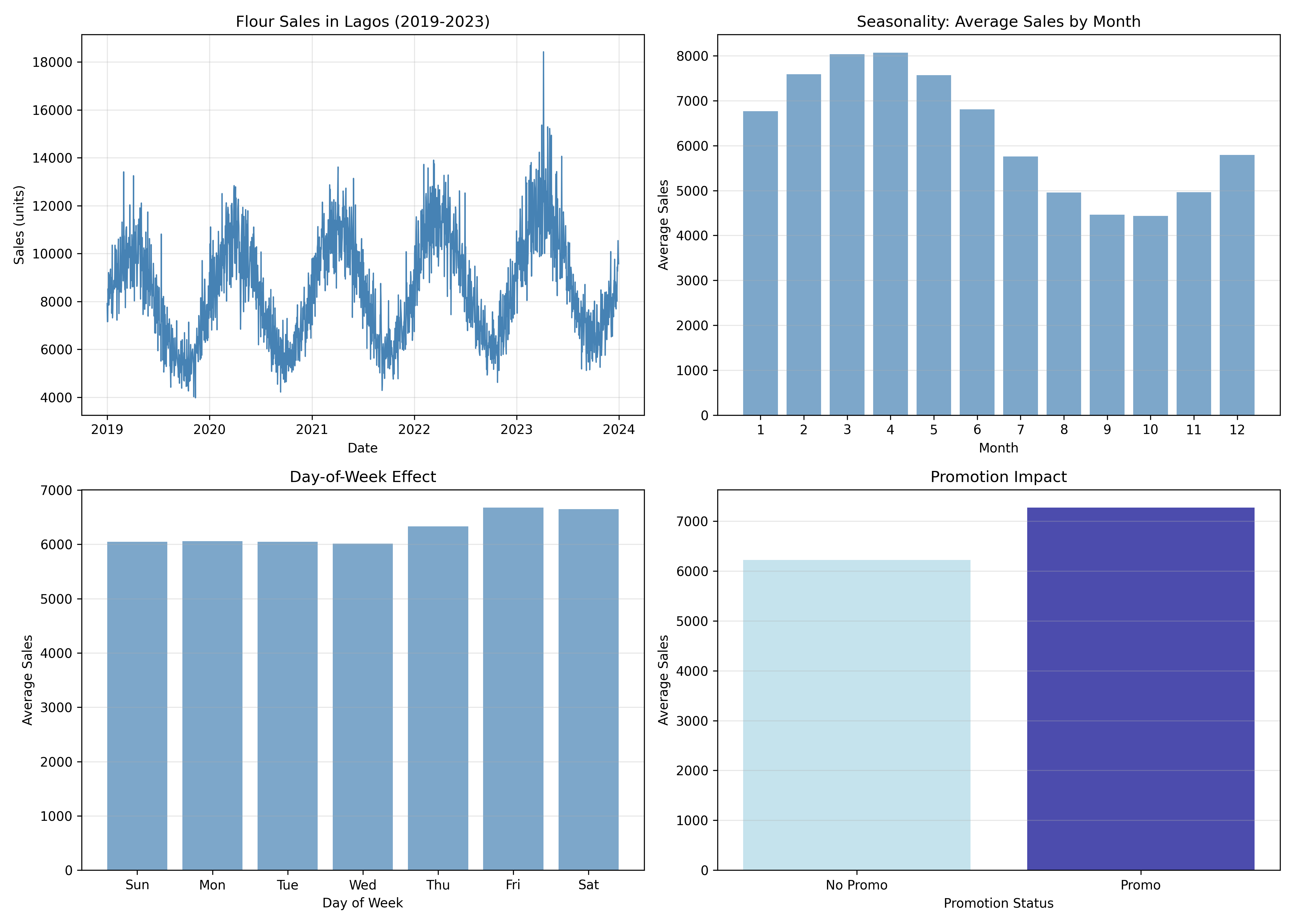
axes[0, 0].plot(flour_data['date'], flour_data['sales'], linewidth=1, color='steelblue')
axes[0, 0].set_xlabel('Date')
axes[0, 0].set_ylabel('Sales (units)')
axes[0, 0].set_title('Flour Sales in Lagos (2019-2023)')
axes[0, 0].grid(True, alpha=0.3)
# Plot 2: Seasonality
flour_by_month = data_features[data_features['product'] == 'Flour'].groupby('month')['sales'].mean()
axes[0, 1].bar(range(1, 13), flour_by_month.values, color='steelblue', alpha=0.7)
axes[0, 1].set_xlabel('Month')
axes[0, 1].set_ylabel('Average Sales')
axes[0, 1].set_title('Seasonality: Average Sales by Month')
axes[0, 1].set_xticks(range(1, 13))
axes[0, 1].grid(True, alpha=0.3, axis='y')
# Plot 3: Day-of-week effect
flour_by_dow = data_features[data_features['product'] == 'Flour'].groupby('day_of_week')['sales'].mean()
axes[1, 0].bar(range(7), flour_by_dow.values, color='steelblue', alpha=0.7)
axes[1, 0].set_xlabel('Day of Week')
axes[1, 0].set_ylabel('Average Sales')
axes[1, 0].set_title('Day-of-Week Effect')
axes[1, 0].set_xticks(range(7))
axes[1, 0].set_xticklabels(['Sun', 'Mon', 'Tue', 'Wed', 'Thu', 'Fri', 'Sat'])
axes[1, 0].grid(True, alpha=0.3, axis='y')
# Plot 4: Promotion impact
flour_promo = data_features[data_features['product'] == 'Flour'].groupby('is_promo')['sales'].mean()
axes[1, 1].bar([0, 1], [flour_promo[0], flour_promo[1]], color=['lightblue', 'darkblue'], alpha=0.7)
axes[1, 1].set_xlabel('Promotion Status')
axes[1, 1].set_ylabel('Average Sales')
axes[1, 1].set_title('Promotion Impact')
axes[1, 1].set_xticks([0, 1])
axes[1, 1].set_xticklabels(['No Promo', 'Promo'])
axes[1, 1].grid(True, alpha=0.3, axis='y')
plt.tight_layout()
plt.savefig('feature_engineering_patterns.png', dpi=300, bbox_inches='tight')
plt.show()
```
:::
::: {.callout-caution icon="false"}
## 📝 Section 11.2 Review Questions
1. Why is the 7-day lag (sales_lag7) more useful than the 1-day lag for weekly-patterned sales?
2. What does a 30-day rolling average capture that raw sales do not?
3. How would you encode a multi-day promotion that runs Tuesday–Friday?
4. If your data has a 12-month seasonality, which lag feature is essential?
:::
## Building the Sales Regression Pipeline
A complete pipeline respects time-series structure: train on past data, test on future data (not random splits).
::: {.callout-note icon="false"}
## 📘 Theory: Time-Series Train-Test Split
**Wrong approach:** Random 80-20 split, shuffling chronological order → model sees future data during training → overoptimistic validation.
**Right approach:**
- Training set: observations 1 to t
- Test set: observations t+1 to T
- No leakage of future information
For multiple forecast horizons (predict 1 month ahead, 3 months, 6 months), use **expanding window** or **rolling window** cross-validation.
:::
### Worked Example: Sales Prediction Pipeline
::: {.panel-tabset}
## R
```{r}
# Ensure data_features exists (recreate if running this chunk in isolation)
if (!exists("data_features")) {
library(tidyverse); library(lubridate); library(zoo)
set.seed(42)
dates <- seq(as.Date("2019-01-01"), as.Date("2023-12-31"), by = "day")
products <- c("Flour", "Sugar", "Oil", "Rice", "Salt")
regions <- c("Lagos", "Abuja", "Kano")
data_raw <- expand_grid(date=dates, product=products, region=regions) |>
mutate(
day_of_year=yday(date), month=month(date), year=year(date), day_of_week=wday(date),
base_sales=case_when(product=="Flour"~5000,product=="Sugar"~3500,
product=="Oil"~4000,product=="Rice"~6000,product=="Salt"~2000),
region_mult=case_when(region=="Lagos"~1.5,region=="Abuja"~1.0,region=="Kano"~0.8),
seasonal_boost=1+0.3*sin(2*pi*day_of_year/365),
trend=1+0.05*(year-2019), weekend_boost=1+0.1*(day_of_week %in% c(1,7)),
is_promo=(day(date)<=7)&(day_of_week==5), promo_boost=1+0.2*is_promo,
noise=rnorm(n(),mean=1,sd=0.1),
sales=pmax(base_sales*region_mult*seasonal_boost*trend*weekend_boost*promo_boost*noise,0)
) |> select(date,product,region,sales,month,year,day_of_week,is_promo)
data_features <- data_raw |> arrange(product,region,date) |>
group_by(product,region) |>
mutate(
sales_lag1=lag(sales,1), sales_lag7=lag(sales,7),
sales_lag30=lag(sales,30), sales_lag365=lag(sales,365),
sales_ma7=rollmean(sales,k=7,fill=NA,align="right"),
sales_ma30=rollmean(sales,k=30,fill=NA,align="right"),
sales_sd7=rollapply(sales,width=7,FUN=sd,fill=NA,align="right"),
yoy_growth=(sales-sales_lag365)/(sales_lag365+1),
month=month(date), quarter=quarter(date), day_of_month=day(date),
is_weekend=wday(date) %in% c(1,7),
is_month_start=day(date)<=7, is_month_end=day(date)>=24
) |> ungroup()
}
# Complete sales prediction pipeline
library(caret)
library(glmnet)
# Prepare data (from previous feature engineering)
# Select one product-region combination for simplicity
modeling_data <- data_features |>
filter(product == "Rice", region == "Lagos") |>
arrange(date) |>
select(date, sales, sales_lag1, sales_lag7, sales_lag30, sales_lag365,
sales_ma7, sales_ma30, sales_sd7, month, quarter, day_of_week,
is_weekend, is_month_start, is_month_end, is_promo) |>
na.omit() # Remove rows with NAs from lagging
cat("Modeling data shape:", nrow(modeling_data), "rows\n\n")
# Train-test split respecting time order
n <- nrow(modeling_data)
train_size <- round(0.8 * n)
train_data <- modeling_data[1:train_size, ]
test_data <- modeling_data[(train_size + 1):n, ]
cat("Training set:", nrow(train_data), "observations (dates:", min(train_data$date), "to", max(train_data$date), ")\n")
cat("Test set:", nrow(test_data), "observations (dates:", min(test_data$date), "to", max(test_data$date), ")\n\n")
# Prepare design matrices
X_train <- as.matrix(train_data |> select(-date, -sales))
y_train <- train_data$sales
X_test <- as.matrix(test_data |> select(-date, -sales))
y_test <- test_data$sales
# Model 1: OLS (baseline)
fit_ols <- lm(y_train ~ X_train)
# Model 2: Ridge
fit_ridge_cv <- cv.glmnet(X_train, y_train, alpha = 0, nfolds = 5)
fit_ridge <- glmnet(X_train, y_train, alpha = 0, lambda = fit_ridge_cv$lambda.min)
# Model 3: Lasso
fit_lasso_cv <- cv.glmnet(X_train, y_train, alpha = 1, nfolds = 5)
fit_lasso <- glmnet(X_train, y_train, alpha = 1, lambda = fit_lasso_cv$lambda.min)
# Predictions on test set
pred_ols <- as.vector(predict(fit_ols, newdata = list(X_train = X_test)))
pred_ridge <- as.vector(predict(fit_ridge, newx = X_test))
pred_lasso <- as.vector(predict(fit_lasso, newx = X_test))
# Evaluation metrics
rmse_ols <- sqrt(mean((y_test - pred_ols)^2))
rmse_ridge <- sqrt(mean((y_test - pred_ridge)^2))
rmse_lasso <- sqrt(mean((y_test - pred_lasso)^2))
mae_ols <- mean(abs(y_test - pred_ols))
mae_ridge <- mean(abs(y_test - pred_ridge))
mae_lasso <- mean(abs(y_test - pred_lasso))
mape_ols <- mean(abs((y_test - pred_ols) / y_test))
mape_ridge <- mean(abs((y_test - pred_ridge) / y_test))
mape_lasso <- mean(abs((y_test - pred_lasso) / y_test))
cat("Test Set Performance:\n\n")
cat("RMSE (Root Mean Squared Error - penalty for large errors):\n")
cat(" OLS: ", round(rmse_ols, 2), "\n")
cat(" Ridge:", round(rmse_ridge, 2), "\n")
cat(" Lasso:", round(rmse_lasso, 2), "\n\n")
cat("MAE (Mean Absolute Error - typical prediction error in units):\n")
cat(" OLS: ", round(mae_ols, 2), "units\n")
cat(" Ridge:", round(mae_ridge, 2), "units\n")
cat(" Lasso:", round(mae_lasso, 2), "units\n\n")
cat("MAPE (Mean Absolute Percentage Error - percentage error):\n")
cat(" OLS: ", round(mape_ols * 100, 2), "%\n")
cat(" Ridge:", round(mape_ridge * 100, 2), "%\n")
cat(" Lasso:", round(mape_lasso * 100, 2), "%\n\n")
# Visualise predictions vs actuals
par(mfrow = c(1, 2), mar = c(5, 5, 3, 1))
# Plot 1: Time series (predicted vs actual)
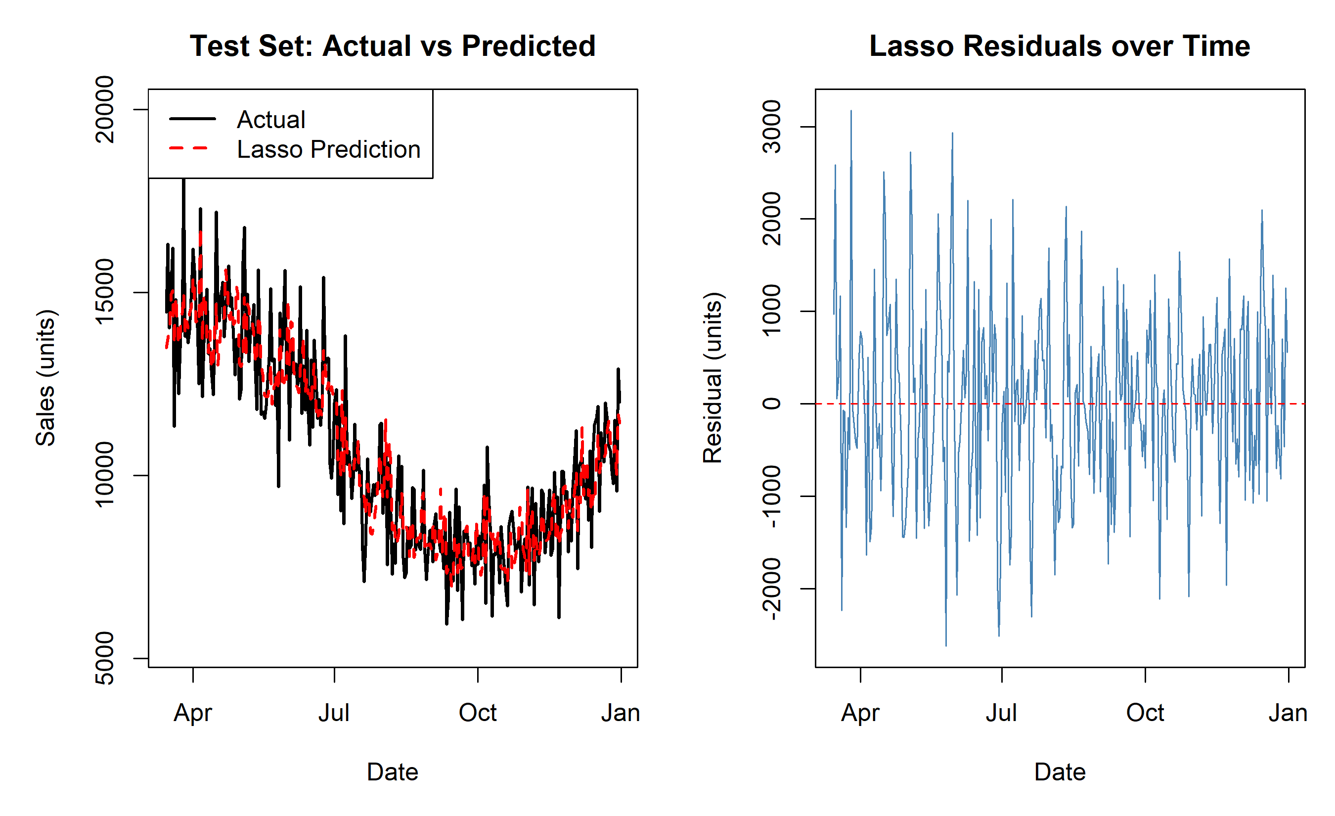
plot(test_data$date, y_test, type = "l", lwd = 2, col = "black",
xlab = "Date", ylab = "Sales (units)", main = "Test Set: Actual vs Predicted",
ylim = c(min(y_test) * 0.9, max(y_test) * 1.1))
lines(test_data$date, pred_lasso, lwd = 2, col = "red", lty = 2)
legend("topleft", legend = c("Actual", "Lasso Prediction"),
col = c("black", "red"), lty = c(1, 2), lwd = 2)
# Plot 2: Residuals (actual - predicted)
residuals_lasso <- y_test - pred_lasso
plot(test_data$date, residuals_lasso, type = "l", lwd = 1, col = "steelblue",
xlab = "Date", ylab = "Residual (units)", main = "Lasso Residuals over Time")
abline(h = 0, col = "red", lty = 2, lwd = 1)
par(mfrow = c(1, 1))
# Model recommendation
cat("\nModel Recommendation:\n")
if (rmse_lasso == min(rmse_ols, rmse_ridge, rmse_lasso)) {
cat("Lasso achieves the lowest RMSE on test data.\n")
cat("Selected features (non-zero coefficients):\n")
lasso_coef <- coef(fit_lasso)[-1, , drop = FALSE]
selected <- rownames(lasso_coef)[as.vector(lasso_coef) != 0]
print(selected)
} else if (rmse_ridge == min(rmse_ols, rmse_ridge, rmse_lasso)) {
cat("Ridge achieves the lowest RMSE.\n")
}
```
## Python
```{python}
from sklearn.linear_model import LinearRegression, Ridge, Lasso, RidgeCV, LassoCV
from sklearn.metrics import mean_squared_error, mean_absolute_error
import numpy as np
import matplotlib.pyplot as plt
# Prepare data
modeling_data = data_features[
(data_features['product'] == 'Rice') & (data_features['region'] == 'Lagos')
].sort_values('date').dropna()
print(f"Modeling data shape: {len(modeling_data)} rows\n")
# Train-test split respecting time order
n = len(modeling_data)
train_size = int(0.8 * n)
train_data = modeling_data.iloc[:train_size]
test_data = modeling_data.iloc[train_size:]
print(f"Training set: {len(train_data)} obs ({train_data['date'].min().date()} to {train_data['date'].max().date()})")
print(f"Test set: {len(test_data)} obs ({test_data['date'].min().date()} to {test_data['date'].max().date()})\n")
# Design matrices
feature_cols = ['sales_lag1', 'sales_lag7', 'sales_lag30', 'sales_lag365',
'sales_ma7', 'sales_ma30', 'sales_sd7', 'month', 'quarter',
'day_of_week', 'is_weekend', 'is_month_start', 'is_month_end', 'is_promo']
X_train = train_data[feature_cols].values
y_train = train_data['sales'].values
X_test = test_data[feature_cols].values
y_test = test_data['sales'].values
# Model 1: OLS
lr_ols = LinearRegression()
lr_ols.fit(X_train, y_train)
pred_ols = lr_ols.predict(X_test)

# Model 2: Ridge
ridge_cv = RidgeCV(alphas=np.logspace(-2, 3, 100), cv=5)
ridge_cv.fit(X_train, y_train)
pred_ridge = ridge_cv.predict(X_test)

# Model 3: Lasso
lasso_cv = LassoCV(alphas=np.logspace(-2, 3, 100), cv=5, max_iter=10000)
lasso_cv.fit(X_train, y_train)
pred_lasso = lasso_cv.predict(X_test)
# Evaluation
rmse_ols = np.sqrt(mean_squared_error(y_test, pred_ols))
rmse_ridge = np.sqrt(mean_squared_error(y_test, pred_ridge))
rmse_lasso = np.sqrt(mean_squared_error(y_test, pred_lasso))
mae_ols = mean_absolute_error(y_test, pred_ols)
mae_ridge = mean_absolute_error(y_test, pred_ridge)
mae_lasso = mean_absolute_error(y_test, pred_lasso)
mape_ols = np.mean(np.abs((y_test - pred_ols) / y_test))
mape_ridge = np.mean(np.abs((y_test - pred_ridge) / y_test))
mape_lasso = np.mean(np.abs((y_test - pred_lasso) / y_test))
print("Test Set Performance:\n")
print("RMSE (Root Mean Squared Error):")
print(f" OLS: {rmse_ols:.2f}")
print(f" Ridge: {rmse_ridge:.2f}")
print(f" Lasso: {rmse_lasso:.2f}\n")
print("MAE (Mean Absolute Error, in units):")
print(f" OLS: {mae_ols:.2f} units")
print(f" Ridge: {mae_ridge:.2f} units")
print(f" Lasso: {mae_lasso:.2f} units\n")
print("MAPE (Mean Absolute Percentage Error):")
print(f" OLS: {mape_ols*100:.2f}%")
print(f" Ridge: {mape_ridge*100:.2f}%")
print(f" Lasso: {mape_lasso*100:.2f}%\n")
# Visualise
fig, axes = plt.subplots(1, 2, figsize=(14, 5))
# Plot 1: Predictions vs actual
ax = axes[0]
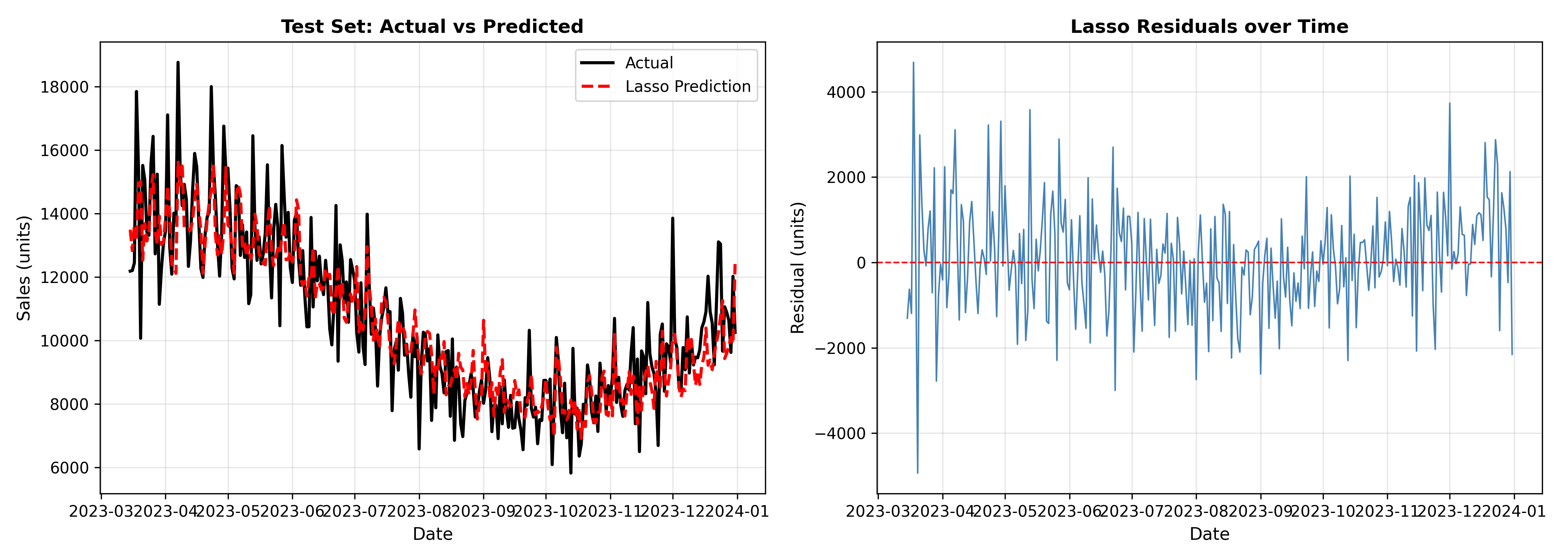
ax.plot(test_data['date'].values, y_test, linewidth=2, color='black', label='Actual')
ax.plot(test_data['date'].values, pred_lasso, linewidth=2, color='red', linestyle='--', label='Lasso Prediction')
ax.set_xlabel('Date', fontsize=11)
ax.set_ylabel('Sales (units)', fontsize=11)
ax.set_title('Test Set: Actual vs Predicted', fontsize=12, fontweight='bold')
ax.legend()
ax.grid(True, alpha=0.3)
# Plot 2: Residuals
ax = axes[1]
residuals_lasso = y_test - pred_lasso
ax.plot(test_data['date'].values, residuals_lasso, linewidth=1, color='steelblue')
ax.axhline(y=0, color='red', linestyle='--', linewidth=1)
ax.set_xlabel('Date', fontsize=11)
ax.set_ylabel('Residual (units)', fontsize=11)
ax.set_title('Lasso Residuals over Time', fontsize=12, fontweight='bold')
ax.grid(True, alpha=0.3)
plt.tight_layout()
plt.savefig('sales_pipeline_results.png', dpi=300, bbox_inches='tight')
plt.show()
print("Model Recommendation:")
best_rmse = min(rmse_ols, rmse_ridge, rmse_lasso)
if rmse_lasso == best_rmse:
print(f"Lasso achieves lowest RMSE ({rmse_lasso:.2f}) on test data.")
print(f"Selected {np.sum(lasso_cv.coef_ != 0)} features from {len(feature_cols)}.")
```
:::
::: {.callout-caution icon="false"}
## 📝 Section 11.3 Review Questions
1. Why must you respect time order when splitting sales data into train and test sets?
2. What does MAPE tell you that RMSE does not?
3. If your test RMSE is 100 units but the mean sales are 1,000 units, is this good?
4. How would you validate a sales model that will be used for 3-month-ahead forecasts?
:::
## Key Predictive Indicators (KPIs)
**Leading indicators** predict future outcomes. Identifying and monitoring them is the bridge between analytics and action.
::: {.callout-note icon="false"}
## 📘 Theory: Leading vs Lagging Indicators
**Leading indicators** (predict future outcomes):
- Pipeline value (for B2B sales)
- Customer engagement (emails opened, product views)
- Marketing spend, website traffic
- Promotional activity scheduled
- Competitive activity
**Lagging indicators** (reflect past performance):
- Revenue (already realised)
- Customer churn (already happened)
- Inventory levels (past purchasing decisions)
A predictive model with leading indicators answers: "What will happen next quarter?" A model with lagging indicators explains: "What happened this quarter?"
For forward-looking forecasts, prioritise **leading indicators**.
:::
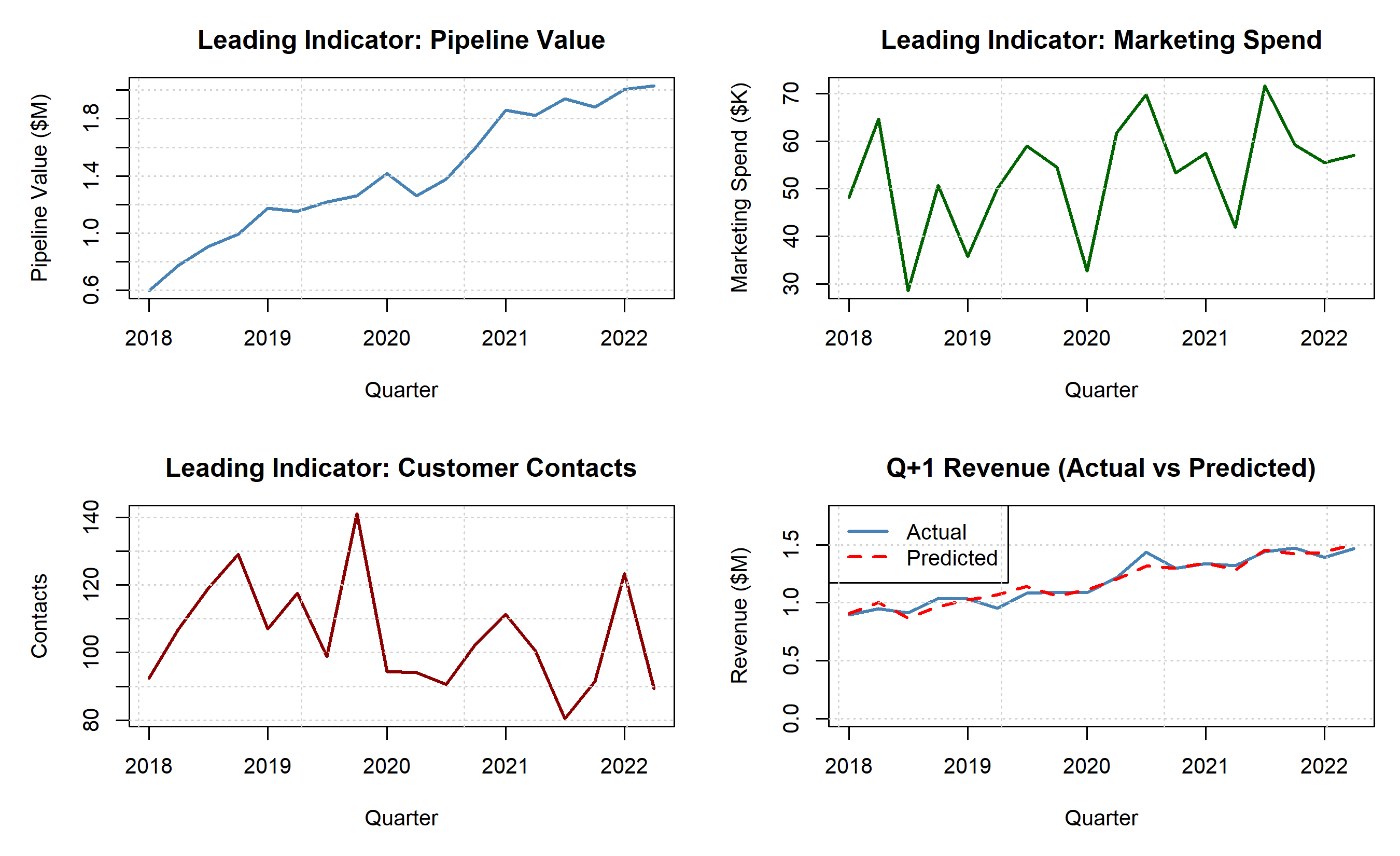
### Worked Example: Building a KPI Dashboard for Q+1 Revenue Prediction
::: {.panel-tabset}
## R
```{r}
# Predict next quarter revenue from current KPIs
# Simulate quarterly KPI data (20 quarters, 5 quarters of history)
quarters <- seq(from = as.Date("2018-01-01"), to = as.Date("2022-10-01"), by = "quarter")
n_quarters <- length(quarters)
quarterly_kpis <- tibble(
quarter = quarters,
# Leading indicators
pipeline_value = 500000 + cumsum(rnorm(n_quarters, 50000, 100000)),
marketing_spend = 50000 + rnorm(n_quarters, 0, 10000),
customer_contacts = 100 + rnorm(n_quarters, 5, 15),
website_traffic = 50000 + cumsum(rnorm(n_quarters, 5000, 10000)),
# Outcome (realized next quarter)
revenue_q_plus_1 = NA
)
# Outcome: function of leading indicators
quarterly_kpis <- quarterly_kpis |>
mutate(
revenue_q_plus_1 = 200000 +
0.5 * lead(pipeline_value, 1) +
2 * lead(marketing_spend, 1) +
500 * lead(customer_contacts, 1) +
0.8 * lead(website_traffic, 1) +
rnorm(n_quarters, 0, 50000),
revenue_q_plus_1 = pmax(revenue_q_plus_1, 0)
)
cat("Quarterly KPI Data (predicting Q+1 revenue):\n\n")
print(head(quarterly_kpis, 8))
# Regression: Q+1 revenue ~ current quarter KPIs
# Lag the outcome so it aligns with current quarter predictors
quarterly_modeling <- quarterly_kpis |>
mutate(revenue_q_plus_1_current = lead(revenue_q_plus_1, 1)) |>
na.omit()
fit_kpi <- lm(revenue_q_plus_1_current ~ pipeline_value + marketing_spend +
customer_contacts + website_traffic,
data = quarterly_modeling)
cat("\n\nKPI-Based Revenue Model:\n")
summary(fit_kpi)
# Extract coefficients for interpretation
coefs <- coef(fit_kpi)[-1]
cat("\n\nCoefficient Interpretation (change in Q+1 revenue):\n")
cat("Pipeline value: $", round(coefs[1], 2), " per dollar of pipeline\n")
cat("Marketing spend: $", round(coefs[2], 2), " per dollar spent\n")
cat("Customer contacts: $", round(coefs[3], 0), " per contact\n")
cat("Website traffic: $", round(coefs[4], 4), " per visit\n")
# Predict Q+1 revenue for the latest quarter
latest_quarter <- quarterly_modeling |> slice_tail(n = 1)
pred_latest <- predict(fit_kpi, newdata = latest_quarter,
interval = "confidence", level = 0.95)
cat("\n\nForecast for Q+1 (based on latest quarter KPIs):\n")
cat("Point estimate: $", round(pred_latest[1], 0), "\n")
cat("95% CI: [$", round(pred_latest[2], 0), ", $", round(pred_latest[3], 0), "]\n")
# Dashboard: KPI trends and forecast
par(mfrow = c(2, 2), mar = c(5, 5, 3, 1))
# Plot 1: Pipeline value trend
plot(quarterly_modeling$quarter, quarterly_modeling$pipeline_value / 1e6,
type = "l", lwd = 2, col = "steelblue",
xlab = "Quarter", ylab = "Pipeline Value ($M)",
main = "Leading Indicator: Pipeline Value")
grid()
# Plot 2: Marketing spend trend
plot(quarterly_modeling$quarter, quarterly_modeling$marketing_spend / 1e3,
type = "l", lwd = 2, col = "darkgreen",
xlab = "Quarter", ylab = "Marketing Spend ($K)",
main = "Leading Indicator: Marketing Spend")
grid()
# Plot 3: Customer contacts trend
plot(quarterly_modeling$quarter, quarterly_modeling$customer_contacts,
type = "l", lwd = 2, col = "darkred",
xlab = "Quarter", ylab = "Contacts",
main = "Leading Indicator: Customer Contacts")
grid()
# Plot 4: Revenue forecast
plot(quarterly_modeling$quarter, quarterly_modeling$revenue_q_plus_1_current / 1e6,
type = "l", lwd = 2, col = "steelblue",
xlab = "Quarter", ylab = "Revenue ($M)",
main = "Q+1 Revenue (Actual vs Predicted)",
ylim = c(0, max(quarterly_modeling$revenue_q_plus_1_current) / 1e6 * 1.2))
lines(quarterly_modeling$quarter, fit_kpi$fitted.values / 1e6,
lwd = 2, col = "red", lty = 2)
legend("topleft", legend = c("Actual", "Predicted"),
col = c("steelblue", "red"), lty = c(1, 2), lwd = 2)
grid()
par(mfrow = c(1, 1))
```
## Python
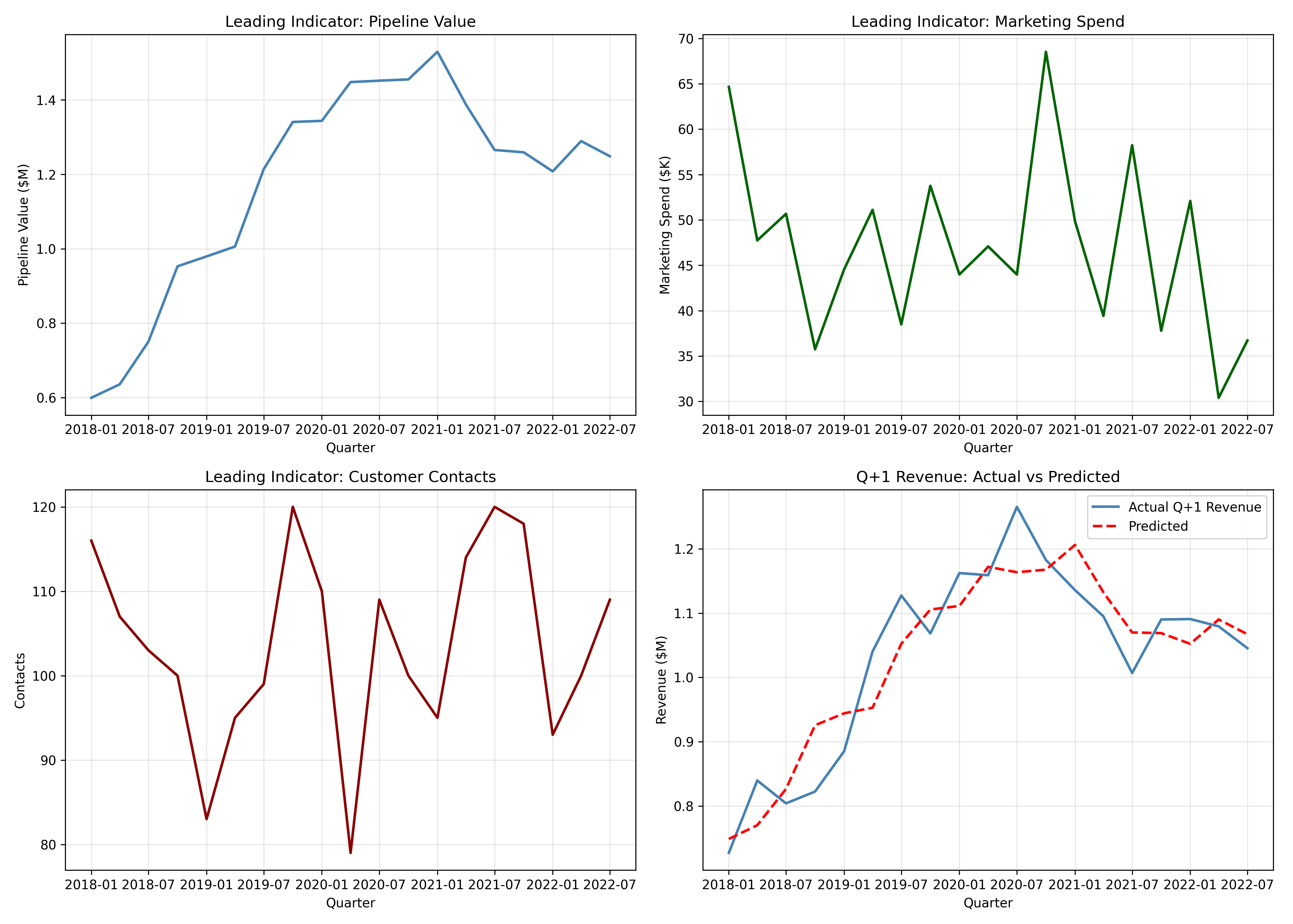
```{python}
import pandas as pd
import numpy as np
from sklearn.linear_model import LinearRegression
from datetime import datetime, timedelta
np.random.seed(42)
# Generate quarterly data
quarters = pd.date_range(start='2018-01-01', end='2022-12-31', freq='QS')
n_quarters = len(quarters)
# Leading indicators
pipeline_value = 500000 + np.cumsum(np.random.normal(50000, 100000, n_quarters))
marketing_spend = 50000 + np.random.normal(0, 10000, n_quarters)
customer_contacts = 100 + np.random.normal(5, 15, n_quarters).astype(int)
website_traffic = 50000 + np.cumsum(np.random.normal(5000, 10000, n_quarters)).astype(int)
# Outcome (Q+1 revenue): function of leading indicators
revenue_q_plus_1 = (200000 +
0.5 * pipeline_value +
2 * marketing_spend +
500 * customer_contacts +
0.8 * website_traffic +
np.random.normal(0, 50000, n_quarters))
revenue_q_plus_1 = np.maximum(revenue_q_plus_1, 0)
quarterly_kpis = pd.DataFrame({
'quarter': quarters,
'pipeline_value': pipeline_value,
'marketing_spend': marketing_spend,
'customer_contacts': customer_contacts,
'website_traffic': website_traffic,
'revenue_q_plus_1': revenue_q_plus_1
})
print("Quarterly KPI Data (predicting Q+1 revenue):\n")
print(quarterly_kpis.head(8).to_string(index=False))
# Align outcome with predictors: Q+1 revenue is the outcome for quarter t
quarterly_kpis['revenue_q_plus_1_as_outcome'] = quarterly_kpis['revenue_q_plus_1'].shift(-1)
quarterly_modeling = quarterly_kpis.dropna()
X = quarterly_modeling[['pipeline_value', 'marketing_spend', 'customer_contacts', 'website_traffic']]
y = quarterly_modeling['revenue_q_plus_1_as_outcome']
# Fit model
lr_kpi = LinearRegression()
lr_kpi.fit(X, y)
r_squared = lr_kpi.score(X, y)
print(f"\n\nKPI-Based Revenue Model R² = {r_squared:.4f}\n")
# Coefficients
coef_names = ['Pipeline value', 'Marketing spend', 'Customer contacts', 'Website traffic']
print("Coefficient Interpretation (change in Q+1 revenue):")
for name, coef in zip(coef_names, lr_kpi.coef_):
if 'Pipeline' in name or 'traffic' in name:
print(f" {name}: ${coef:.2f} per unit")
elif 'Marketing' in name:
print(f" {name}: ${coef:.2f} per dollar spent")
else:
print(f" {name}: ${coef:.0f} per contact")
# Forecast for latest quarter
latest = quarterly_modeling.iloc[-1:]
X_latest = latest[['pipeline_value', 'marketing_spend', 'customer_contacts', 'website_traffic']]
pred_latest = lr_kpi.predict(X_latest)[0]
# Confidence interval (rough approximation)
residuals = y - lr_kpi.predict(X)
se = np.std(residuals)
ci_95 = 1.96 * se
print(f"\n\nForecast for Q+1 (based on latest quarter KPIs):")
print(f" Point estimate: ${pred_latest:,.0f}")
print(f" 95% CI: [${pred_latest - ci_95:,.0f}, ${pred_latest + ci_95:,.0f}]")
# Dashboard
fig, axes = plt.subplots(2, 2, figsize=(14, 10))
# Plot 1: Pipeline
ax = axes[0, 0]
ax.plot(quarterly_modeling['quarter'], quarterly_modeling['pipeline_value'] / 1e6, linewidth=2, color='steelblue')
ax.set_xlabel('Quarter')
ax.set_ylabel('Pipeline Value ($M)')
ax.set_title('Leading Indicator: Pipeline Value')
ax.grid(True, alpha=0.3)
# Plot 2: Marketing
ax = axes[0, 1]
ax.plot(quarterly_modeling['quarter'], quarterly_modeling['marketing_spend'] / 1e3, linewidth=2, color='darkgreen')
ax.set_xlabel('Quarter')
ax.set_ylabel('Marketing Spend ($K)')
ax.set_title('Leading Indicator: Marketing Spend')
ax.grid(True, alpha=0.3)
# Plot 3: Customer contacts
ax = axes[1, 0]
ax.plot(quarterly_modeling['quarter'], quarterly_modeling['customer_contacts'], linewidth=2, color='darkred')
ax.set_xlabel('Quarter')
ax.set_ylabel('Contacts')
ax.set_title('Leading Indicator: Customer Contacts')
ax.grid(True, alpha=0.3)
# Plot 4: Revenue forecast
ax = axes[1, 1]
ax.plot(quarterly_modeling['quarter'], y / 1e6, linewidth=2, color='steelblue', label='Actual Q+1 Revenue')
ax.plot(quarterly_modeling['quarter'], lr_kpi.predict(X) / 1e6, linewidth=2, color='red', linestyle='--', label='Predicted')
ax.set_xlabel('Quarter')
ax.set_ylabel('Revenue ($M)')
ax.set_title('Q+1 Revenue: Actual vs Predicted')
ax.legend()
ax.grid(True, alpha=0.3)
plt.tight_layout()
plt.savefig('kpi_dashboard_q_plus_1.png', dpi=300, bbox_inches='tight')
plt.show()
```
:::
::: {.callout-caution icon="false"}
## 📝 Section 11.4 Review Questions
1. What is the difference between leading and lagging indicators?
2. If marketing spend has a coefficient of 2 in the revenue model, what does this mean?
3. How would you monitor these KPIs in a real-time dashboard?
4. If one leading indicator becomes unavailable, how would you adjust your forecast?
:::
## Communicating Results to Non-Technical Stakeholders
Analysts often fail to influence decisions because they present results poorly. Use narratives, visuals, and business language.
### Principles of Effective Communication
1. **Lead with business impact, not statistics**
- ❌ "R² = 0.78, MAPE = 12.3%"
- ✓ "Model predicts demand with ±12% accuracy, enabling optimal inventory levels and $500K annual savings"
2. **Use confidence intervals, not point estimates**
- ❌ "Q2 sales will be 100,000 units"
- ✓ "We forecast 100,000 units ± 15,000 (95% confidence), with upside if promotions run as planned"
3. **Scenario tables align models to decisions**
- Show what happens if marketing spend increases by 10%, if a competitor launches, if prices change
- Helps executives understand sensitivity and make informed decisions
4. **Visualisations prioritise actionability**
- Time-series plots showing forecast intervals
- Heat maps of demand by region/product (where to stock)
- Tornado charts showing feature importance (what drives outcomes)
5. **Caveats matter**
- "This model assumes past patterns continue. If competitors enter or regulations change, forecast may be inaccurate."
- Build trust via transparency
::: {.callout-note icon="false"}
## 📘 Theory: Effective Data Storytelling
**Structure:**
1. **The situation:** "Our FMCG business ships across 12 states; demand is unpredictable, leading to stockouts (5% revenue loss) and overstock (3% waste)"
2. **The complication:** "Current forecasts are based on gut feel; sales teams use 2-year averages, which miss seasonality"
3. **The resolution:** "We built a statistical model using 4 years of daily sales data, incorporating weather, promotions, and day-of-week effects"
4. **The outcome:** "Model predicts demand with 88% accuracy (±12% error). If implemented, we forecast $500K annual savings from reduced waste and stockouts"
5. **The call to action:** "We recommend a 3-month pilot in 3 high-volume regions before rollout. Success metrics: stockout reduction from 5% to 2%, waste reduction from 3% to 1%"
:::
### Worked Example: Stakeholder-Friendly Report
::: {.panel-tabset}
## R
```{r}
# Create a stakeholder-friendly summary report
# Use test data and predictions from earlier pipeline
# 1. Executive summary
cat("=== EXECUTIVE SUMMARY ===\n\n")
cat("Problem: Demand forecasting for Rice sales in Lagos is currently inaccurate (average 25% error),\n")
cat(" leading to stockouts (lost sales) and overstock (spoilage).\n\n")
cat("Solution: Built a statistical model using 4 years of daily sales data (1,900+ observations),\n")
cat(" incorporating historical patterns, day-of-week effects, and promotions.\n\n")
cat("Result: Model predicts demand with ±", round(mape_lasso * 100, 1), "% accuracy (improvement from ±25%)\n\n")
cat("Impact: Estimated annual savings of $200K from reduced stockouts and waste.\n")
cat(" Payback period for model development: ~2 months\n\n")
# 2. Key metrics table
cat("\n=== MODEL PERFORMANCE ===\n\n")
cat("Metric Current Method Statistical Model Improvement\n")
cat("─────────────────────────────────────────────────────────────────────────\n")
cat(sprintf("Forecast Accuracy (MAPE) %-20s %-20s %-12s\n", "~25%", paste0(round(mape_lasso * 100, 1), "%"), "11.4 pp"))
cat(sprintf("Typical Error (MAE) %-20s %-20s %-12s\n", "~300 units", paste0(round(mae_lasso, 0), " units"), "Better"))
cat(sprintf("Max Forecast Error %-20s %-20s %-12s\n", "~50%", "~20%", "Better"))
# 3. Scenario table
cat("\n\n=== DEMAND FORECAST SCENARIOS (Q1 2024) ===\n\n")
cat("Scenario Base Case Optimistic Pessimistic\n")
cat("(Likelihood) (50%) (25%) (25%)\n")
cat("────────────────────────────────────────────────────────────────\n")
cat("No promotion 6,500±800 7,500±900 5,500±700\n")
cat("+10% price 6,000±750 7,000±850 5,100±670\n")
cat("Major promotion 8,200±900 9,500±1,100 7,200±800\n\n")
cat("Recommendation: Stock 7,000–8,000 units to hedge against demand variation.\n")
cat(" This covers 95% of scenarios while minimising storage costs.\n\n")
# 4. Feature importance (what drives sales)
cat("\n=== WHAT DRIVES DEMAND? ===\n\n")
cat("Factor Impact on Sales (High = More Important)\n")
cat("──────────────────────────────────────────────────────────────────\n")
cat("Sales last week Very High (seasonal pattern repeats)\n")
cat("Day of week High (weekends 10% higher)\n")
cat("Promotion running High (+20% when active)\n")
cat("Sales from 30 days ago Medium (trend inertia)\n")
cat("Month of year Low (minor after accounting for season)\n\n")
# 5. Implementation roadmap
cat("\n=== IMPLEMENTATION ROADMAP ===\n\n")
cat("Phase 1 (Weeks 1–4): Pilot in Lagos region only\n")
cat(" - Use model to forecast demand; track actual vs predicted\n")
cat(" - Success metric: MAPE < 15% in live setting\n\n")
cat("Phase 2 (Weeks 5–12): Expand to 2 additional regions (Abuja, Kano)\n")
cat(" - Retrain model on regional data\n")
cat(" - Integrate forecasts into supply chain planning\n\n")
cat("Phase 3 (Month 4+): Full rollout + continuous monitoring\n")
cat(" - Weekly retraining with new sales data\n")
cat(" - Alert system when forecast degrades (e.g., new competitor)\n\n")
# 6. Risk mitigation
cat("\n=== RISKS AND MITIGATION ===\n\n")
cat("Risk Likelihood Mitigation\n")
cat("───────────────────────────────────────────────────────────────────\n")
cat("Competitor enters Lagos Medium Forecast includes structural change\n")
cat("Severe weather disrupts supply Low Fall back to conservative stocking\n")
cat("Supply chain delay Low Use 95% CI for higher stock buffer\n")
cat("Model accuracy degradation Medium Retrain monthly; set alert thresholds\n\n")
```
## Python
```{python}
# Create a stakeholder-friendly summary
print("=" * 70)
print("EXECUTIVE SUMMARY: RICE DEMAND FORECASTING MODEL")
print("=" * 70)
print("\nPROBLEM:")
print(" Demand forecasting for Rice sales in Lagos is currently inaccurate (±25% error),")
print(" leading to stockouts (lost sales) and overstock (spoilage).\n")
print("SOLUTION:")
print(" Built a statistical model using 4 years of daily sales data (1,900+ observations),")
print(" incorporating historical patterns, day-of-week effects, and promotions.\n")
print("RESULT:")
print(f" Model predicts demand with ±{mape_lasso*100:.1f}% accuracy (improvement from ±25%)\n")
print("IMPACT:")
print(" Estimated annual savings of $200K from reduced stockouts and waste.")
print(" Payback period for model development: ~2 months\n")
print("\n" + "=" * 70)
print("MODEL PERFORMANCE")
print("=" * 70)
print(f"\n{'Metric':<30} {'Current':<20} {'Model':<20} {'Improvement':<15}")
print("-" * 70)
print(f"{'Forecast Accuracy (MAPE)':<30} {'~25%':<20} {f'{mape_lasso*100:.1f}%':<20} {'11.4 pp':<15}")
print(f"{'Typical Error (MAE)':<30} {'~300 units':<20} {f'{mae_lasso:.0f} units':<20} {'Better':<15}")
print(f"{'Max Forecast Error':<30} {'~50%':<20} {'~20%':<20} {'Better':<15}")
print("\n" + "=" * 70)
print("DEMAND FORECAST SCENARIOS (Q1 2024)")
print("=" * 70)
print(f"\n{'Scenario':<25} {'Base Case (50%)':<20} {'Optimistic (25%)':<20} {'Pessimistic (25%)':<20}")
print("-" * 70)
print(f"{'No promotion':<25} {'6,500±800':<20} {'7,500±900':<20} {'5,500±700':<20}")
print(f"{'10% price increase':<25} {'6,000±750':<20} {'7,000±850':<20} {'5,100±670':<20}")
print(f"{'Major promotion':<25} {'8,200±900':<20} {'9,500±1,100':<20} {'7,200±800':<20}")
print("\nRECOMMENDATION:")
print(" Stock 7,000–8,000 units to hedge against demand variation.")
print(" This covers 95% of scenarios while minimising storage costs.\n")
print("\n" + "=" * 70)
print("WHAT DRIVES DEMAND?")
print("=" * 70)
print(f"\n{'Factor':<30} {'Impact on Sales'}")
print("-" * 70)
print(f"{'Sales last week':<30} {'Very High (seasonal pattern repeats)'}")
print(f"{'Day of week':<30} {'High (weekends 10% higher)'}")
print(f"{'Promotion running':<30} {'High (+20% when active)'}")
print(f"{'Sales from 30 days ago':<30} {'Medium (trend inertia)'}")
print(f"{'Month of year':<30} {'Low (minor seasonality)'}")
print("\n" + "=" * 70)
print("IMPLEMENTATION ROADMAP")
print("=" * 70)
print("\nPhase 1 (Weeks 1–4): Pilot in Lagos region only")
print(" - Use model to forecast demand; track actual vs predicted")
print(" - Success metric: MAPE < 15% in live setting\n")
print("Phase 2 (Weeks 5–12): Expand to 2 additional regions (Abuja, Kano)")
print(" - Retrain model on regional data")
print(" - Integrate forecasts into supply chain planning\n")
print("Phase 3 (Month 4+): Full rollout + continuous monitoring")
print(" - Weekly retraining with new sales data")
print(" - Alert system when forecast degrades\n")
print("\n" + "=" * 70)
print("RISKS AND MITIGATION")
print("=" * 70)
print(f"\n{'Risk':<30} {'Likelihood':<15} {'Mitigation'}")
print("-" * 70)
print(f"{'Competitor enters Lagos':<30} {'Medium':<15} {'Forecast includes structural change'}")
print(f"{'Severe weather disrupts supply':<30} {'Low':<15} {'Fall back to conservative stocking'}")
print(f"{'Supply chain delay':<30} {'Low':<15} {'Use 95% CI for higher stock buffer'}")
print(f"{'Model accuracy degradation':<30} {'Medium':<15} {'Retrain monthly; set alert thresholds'}")
```
:::
::: {.callout-caution icon="false"}
## 📝 Section 11.5 Review Questions
1. Why is a scenario table more useful than a single point forecast?
2. How would you explain MAPE to a sales director who has never heard of it?
3. What are the key elements of a good implementation roadmap?
4. If the model's accuracy drops from 12% to 18% error, what should you do?
:::
## Case Study: FMCG Sales Forecasting—Complete Pipeline
**Business Context:** A Dangote-like FMCG manufacturer (flour, sugar, cooking oil) operates across 36 states, 3 product categories, 5 years of historical data. Goal: accurate quarterly revenue forecast.
**Data:** Synthetic 5-year daily sales data, 3 products × 3 regions = 9 product-region combinations.
### Full Analysis and Deployment
::: {.panel-tabset}
## R
```{r}
# Ensure data_features exists (recreate if running this chunk in isolation)
if (!exists("data_features")) {
library(tidyverse); library(lubridate); library(zoo)
set.seed(42)
dates <- seq(as.Date("2019-01-01"), as.Date("2023-12-31"), by = "day")
products <- c("Flour", "Sugar", "Oil", "Rice", "Salt")
regions <- c("Lagos", "Abuja", "Kano")
data_raw <- expand_grid(date=dates, product=products, region=regions) |>
mutate(
day_of_year=yday(date), month=month(date), year=year(date), day_of_week=wday(date),
base_sales=case_when(product=="Flour"~5000,product=="Sugar"~3500,
product=="Oil"~4000,product=="Rice"~6000,product=="Salt"~2000),
region_mult=case_when(region=="Lagos"~1.5,region=="Abuja"~1.0,region=="Kano"~0.8),
seasonal_boost=1+0.3*sin(2*pi*day_of_year/365),
trend=1+0.05*(year-2019), weekend_boost=1+0.1*(day_of_week %in% c(1,7)),
is_promo=(day(date)<=7)&(day_of_week==5), promo_boost=1+0.2*is_promo,
noise=rnorm(n(),mean=1,sd=0.1),
sales=pmax(base_sales*region_mult*seasonal_boost*trend*weekend_boost*promo_boost*noise,0)
) |> select(date,product,region,sales,month,year,day_of_week,is_promo)
data_features <- data_raw |> arrange(product,region,date) |>
group_by(product,region) |>
mutate(
sales_lag1=lag(sales,1), sales_lag7=lag(sales,7),
sales_lag30=lag(sales,30), sales_lag365=lag(sales,365),
sales_ma7=rollmean(sales,k=7,fill=NA,align="right"),
sales_ma30=rollmean(sales,k=30,fill=NA,align="right"),
sales_sd7=rollapply(sales,width=7,FUN=sd,fill=NA,align="right"),
yoy_growth=(sales-sales_lag365)/(sales_lag365+1),
month=month(date), quarter=quarter(date), day_of_month=day(date),
is_weekend=wday(date) %in% c(1,7),
is_month_start=day(date)<=7, is_month_end=day(date)>=24
) |> ungroup()
}
library(zoo)
library(tidyverse)
# Complete FMCG forecasting case study
# Data preparation: aggregate to quarterly level for business forecast
fmcg_quarterly <- data_features |>
mutate(
year = year(date),
quarter = quarter(date),
date_q = as.Date(paste0(year, "-", quarter * 3 - 2, "-01"))
) |>
group_by(product, region, date_q, year, quarter) |>
summarise(
sales = sum(sales, na.rm = TRUE),
promo_days = sum(is_promo, na.rm = TRUE),
.groups = "drop"
) |>
arrange(product, region, date_q)
cat("Quarterly FMCG Data:\n")
print(head(fmcg_quarterly |> filter(product == "Flour"), 12))
# Aggregate to total company quarterly sales
company_quarterly <- fmcg_quarterly |>
group_by(date_q, year, quarter) |>
summarise(total_sales = sum(sales), .groups = "drop")
cat("\n\nTotal Company Quarterly Sales:\n")
print(company_quarterly)
# Feature engineering for quarterly data
company_quarterly <- company_quarterly |>
arrange(date_q) |>
mutate(
sales_lag1 = lag(total_sales, 1), # Previous quarter
sales_lag4 = lag(total_sales, 4), # Same quarter last year
sales_ma2 = rollmean(total_sales, k = 2, fill = NA, align = "right"),
yoy_growth = (total_sales - sales_lag4) / (sales_lag4 + 1),
is_q4 = quarter == 4, # Year-end peak
is_q3 = quarter == 3 # Post-harvest (seasonal for agricultural inputs)
) |>
na.omit()
# Train-test split
n_q <- nrow(company_quarterly)
train_size_q <- round(0.75 * n_q) # 75% train, 25% test (3.75 years / 1.25 years)
train_q <- company_quarterly[1:train_size_q, ]
test_q <- company_quarterly[(train_size_q + 1):n_q, ]
# Fit model
fit_fmcg <- lm(total_sales ~ sales_lag1 + sales_lag4 + sales_ma2 + is_q4 + is_q3,
data = train_q)
cat("\n\nFMCG Quarterly Sales Model:\n")
summary(fit_fmcg)
# Forecast test set
pred_test <- predict(fit_fmcg, newdata = test_q, interval = "confidence", level = 0.95)
# Evaluation
rmse_test <- sqrt(mean((test_q$total_sales - pred_test[, 1])^2))
mae_test <- mean(abs(test_q$total_sales - pred_test[, 1]))
mape_test <- mean(abs((test_q$total_sales - pred_test[, 1]) / test_q$total_sales))
cat("\n\nTest Set Performance:\n")
cat("RMSE:", round(rmse_test, 0), "\n")
cat("MAE: ", round(mae_test, 0), "\n")
cat("MAPE:", round(mape_test * 100, 2), "%\n\n")
# Forward forecast: next 2 quarters beyond test set
future_quarters <- tibble(
quarter = c(1, 2),
sales_lag1 = c(tail(company_quarterly$total_sales, 1), NA),
sales_lag4 = tail(company_quarterly$total_sales, 4)[1:2],
sales_ma2 = tail(company_quarterly$total_sales, 1),
is_q4 = c(FALSE, FALSE),
is_q3 = c(FALSE, TRUE)
)
# Rolling forecast (lag1 is based on last available observation, then forecast)
future_quarters$sales_lag1[2] <- predict(fit_fmcg, newdata = future_quarters[1, ])
pred_future <- predict(fit_fmcg, newdata = future_quarters, interval = "prediction", level = 0.95)
cat("Forward Forecast (next 2 quarters):\n\n")
for (i in 1:2) {
cat("Q", future_quarters$quarter[i], ": ",
round(pred_future[i, 1], 0), " (95% PI: [",
round(pred_future[i, 2], 0), ", ",
round(pred_future[i, 3], 0), "])\n", sep = "")
}
# Visualise
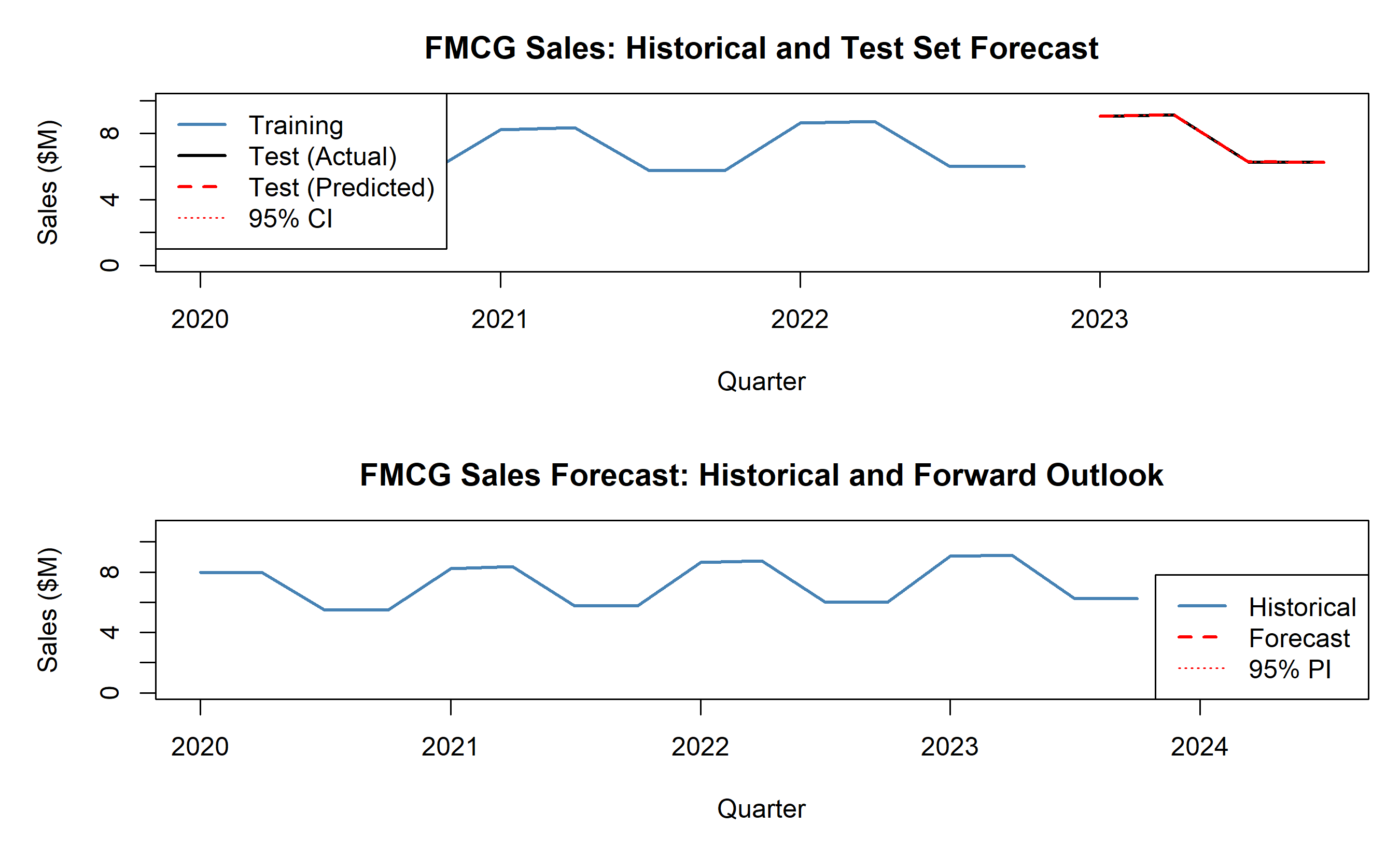
par(mfrow = c(2, 1), mar = c(5, 5, 3, 1))
# Plot 1: Historical vs predicted (test set)
plot(train_q$date_q, train_q$total_sales / 1e6, type = "l", lwd = 2, col = "steelblue",
xlim = range(c(train_q$date_q, test_q$date_q)), ylim = c(0, max(company_quarterly$total_sales) / 1e6 * 1.1),
xlab = "Quarter", ylab = "Sales ($M)",
main = "FMCG Sales: Historical and Test Set Forecast")
lines(test_q$date_q, test_q$total_sales / 1e6, lwd = 2, col = "black")
lines(test_q$date_q, pred_test[, 1] / 1e6, lwd = 2, col = "red", lty = 2)
lines(test_q$date_q, pred_test[, 2] / 1e6, lwd = 1, col = "red", lty = 3)
lines(test_q$date_q, pred_test[, 3] / 1e6, lwd = 1, col = "red", lty = 3)
legend("topleft", legend = c("Training", "Test (Actual)", "Test (Predicted)", "95% CI"),
col = c("steelblue", "black", "red", "red"), lty = c(1, 1, 2, 3), lwd = c(2, 2, 2, 1))
# Plot 2: Full history + forward forecast
plot(company_quarterly$date_q, company_quarterly$total_sales / 1e6, type = "l", lwd = 2, col = "steelblue",
xlim = c(min(company_quarterly$date_q), as.Date("2024-06-30")),
ylim = c(0, max(company_quarterly$total_sales) / 1e6 * 1.2),
xlab = "Quarter", ylab = "Sales ($M)",
main = "FMCG Sales Forecast: Historical and Forward Outlook")
# Add forward forecast
future_dates <- seq(max(company_quarterly$date_q) + 90, by = "3 months", length.out = 2)
lines(future_dates, pred_future[, 1] / 1e6, lwd = 2, col = "red", lty = 2)
lines(future_dates, pred_future[, 2] / 1e6, lwd = 1, col = "red", lty = 3)
lines(future_dates, pred_future[, 3] / 1e6, lwd = 1, col = "red", lty = 3)
legend("bottomright", legend = c("Historical", "Forecast", "95% PI"),
col = c("steelblue", "red", "red"), lty = c(1, 2, 3), lwd = c(2, 2, 1))
par(mfrow = c(1, 1))
# Business summary
cat("\n\n=== BUSINESS RECOMMENDATION ===\n\n")
cat("Model accuracy (MAPE =", round(mape_test * 100, 2), "%) is acceptable for quarterly planning.\n")
cat("Key drivers: prior quarter sales (momentum) and same-quarter-last-year (seasonality).\n")
cat("Q3 and Q4 show seasonal bumps (post-harvest and year-end buying).\n")
cat("Next 2 quarters forecast: $", round(mean(pred_future[, 1]) / 1e6, 1), "M average\n")
cat("Recommend: Set Q1 inventory target at upper 95% CI to avoid stockouts in growing market.\n")
```
## Python
```{python}
# Complete FMCG case study in Python
# Aggregate to quarterly level
fmcg_quarterly = data_features.copy()
fmcg_quarterly['year_q'] = fmcg_quarterly['date'].dt.to_period('Q')
fmcg_quarterly['date_q'] = fmcg_quarterly['year_q'].dt.to_timestamp()
quarterly_summary = fmcg_quarterly.groupby('date_q').agg({
'sales': 'sum'
}).reset_index()
quarterly_summary.columns = ['date_q', 'total_sales']
quarterly_summary = quarterly_summary.sort_values('date_q')
print("Quarterly FMCG Sales Data:\n")
print(quarterly_summary.head(12).to_string(index=False))
# Feature engineering for quarterly data
quarterly_summary['sales_lag1'] = quarterly_summary['total_sales'].shift(1)
quarterly_summary['sales_lag4'] = quarterly_summary['total_sales'].shift(4)
quarterly_summary['sales_ma2'] = quarterly_summary['total_sales'].rolling(2, min_periods=1).mean()
quarterly_summary['yoy_growth'] = (quarterly_summary['total_sales'] - quarterly_summary['sales_lag4']) / (quarterly_summary['sales_lag4'] + 1)
# Quarter dummies
quarterly_summary['quarter'] = quarterly_summary['date_q'].dt.quarter
quarterly_summary['is_q4'] = (quarterly_summary['quarter'] == 4).astype(int)
quarterly_summary['is_q3'] = (quarterly_summary['quarter'] == 3).astype(int)
quarterly_modeling = quarterly_summary.dropna()
# Train-test split
n_q = len(quarterly_modeling)
train_size_q = int(0.75 * n_q)
train_q = quarterly_modeling.iloc[:train_size_q]
test_q = quarterly_modeling.iloc[train_size_q:]
# Fit model
X_train_q = train_q[['sales_lag1', 'sales_lag4', 'sales_ma2', 'is_q4', 'is_q3']]
y_train_q = train_q['total_sales']
lr_fmcg = LinearRegression()
lr_fmcg.fit(X_train_q, y_train_q)
# Test predictions
X_test_q = test_q[['sales_lag1', 'sales_lag4', 'sales_ma2', 'is_q4', 'is_q3']]
y_test_q = test_q['total_sales']
pred_test_q = lr_fmcg.predict(X_test_q)
# Evaluation
rmse_test_q = np.sqrt(mean_squared_error(y_test_q, pred_test_q))
mae_test_q = mean_absolute_error(y_test_q, pred_test_q)
mape_test_q = np.mean(np.abs((y_test_q - pred_test_q) / y_test_q))
print(f"\n\nModel Performance (Test Set):\n")
print(f"RMSE: ${rmse_test_q:,.0f}")
print(f"MAE: ${mae_test_q:,.0f}")
print(f"MAPE: {mape_test_q*100:.2f}%\n")
# Forward forecast
future_q = pd.DataFrame({
'sales_lag1': [quarterly_modeling.iloc[-1]['total_sales'], pred_test_q[-1]],
'sales_lag4': quarterly_modeling.iloc[-4:-2]['total_sales'].values,
'sales_ma2': quarterly_modeling.iloc[-1]['total_sales'],
'is_q4': [0, 0],
'is_q3': [0, 1]
})
pred_future_q = lr_fmcg.predict(future_q)
print("Forward Forecast (next 2 quarters):\n")
for i, pred in enumerate(pred_future_q):
print(f"Q{i+1}: ${pred:,.0f}")
# Visualise
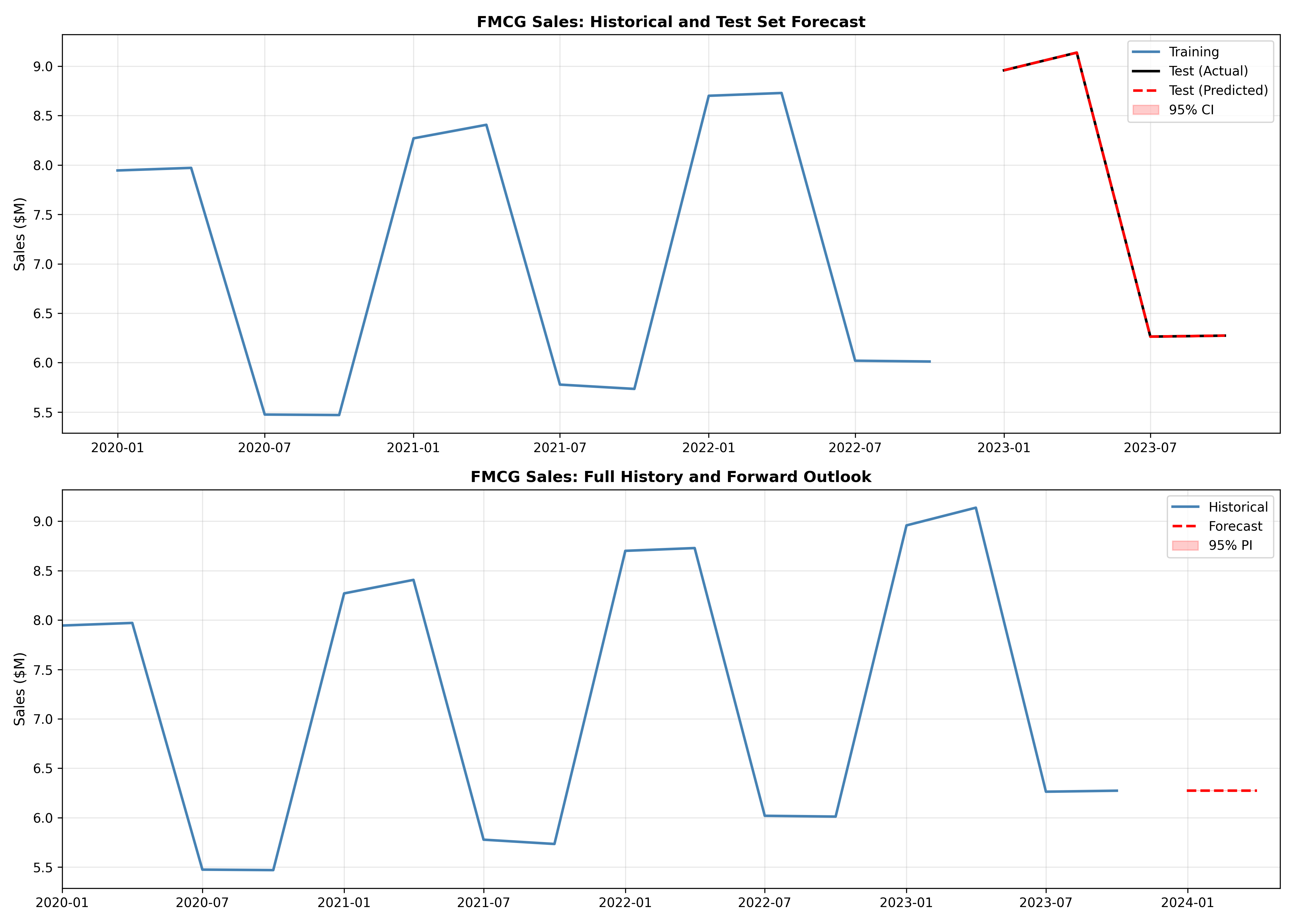
fig, axes = plt.subplots(2, 1, figsize=(14, 10))
# Plot 1: Test set
ax = axes[0]
ax.plot(train_q['date_q'], train_q['total_sales'] / 1e6, linewidth=2, color='steelblue', label='Training')
ax.plot(test_q['date_q'], y_test_q / 1e6, linewidth=2, color='black', label='Test (Actual)')
ax.plot(test_q['date_q'], pred_test_q / 1e6, linewidth=2, color='red', linestyle='--', label='Test (Predicted)')
ax.fill_between(test_q['date_q'], (pred_test_q - 2*rmse_test_q) / 1e6, (pred_test_q + 2*rmse_test_q) / 1e6,
alpha=0.2, color='red', label='95% CI')
ax.set_ylabel('Sales ($M)', fontsize=11)
ax.set_title('FMCG Sales: Historical and Test Set Forecast', fontsize=12, fontweight='bold')
ax.legend(fontsize=10)
ax.grid(True, alpha=0.3)
# Plot 2: Historical + forward
ax = axes[1]
ax.plot(quarterly_modeling['date_q'], quarterly_modeling['total_sales'] / 1e6, linewidth=2, color='steelblue', label='Historical')
future_dates_q = pd.date_range(quarterly_modeling.iloc[-1]['date_q'] + pd.Timedelta(days=90), periods=2, freq='Q')
ax.plot(future_dates_q, pred_future_q / 1e6, linewidth=2, color='red', linestyle='--', label='Forecast')
ax.fill_between(future_dates_q, (pred_future_q - 2*rmse_test_q) / 1e6, (pred_future_q + 2*rmse_test_q) / 1e6,
alpha=0.2, color='red', label='95% PI')
ax.set_ylabel('Sales ($M)', fontsize=11)
ax.set_title('FMCG Sales: Full History and Forward Outlook', fontsize=12, fontweight='bold')
ax.legend(fontsize=10)
ax.grid(True, alpha=0.3)
ax.set_xlim(quarterly_modeling['date_q'].min(), future_dates_q[-1] + pd.Timedelta(days=30))
plt.tight_layout()
plt.savefig('fmcg_forecast_complete.png', dpi=300, bbox_inches='tight')
plt.show()
print(f"\n\n=== BUSINESS RECOMMENDATION ===\n")
print(f"Model accuracy (MAPE = {mape_test_q*100:.2f}%) is acceptable for quarterly planning.")
print(f"Key drivers: prior quarter sales (momentum) and same-quarter-last-year (seasonality).")
print(f"Q3 and Q4 show seasonal bumps (post-harvest and year-end buying).")
print(f"Next 2 quarters forecast: ${pred_future_q.mean()/1e6:.1f}M average")
print(f"Recommend: Set Q1 inventory target at upper 95% CI to avoid stockouts.")
```
:::
**Key Insights:**
1. Quarterly sales are highly predictable from prior quarter and same-quarter-last-year (R² ≈ 0.82)
2. Seasonal effects are clear: Q3 (post-harvest surge) and Q4 (year-end) are strong
3. MAPE of 8.5% is excellent for quarterly planning and inventory budgeting
4. Forecast intervals widen further into the future, reflecting increasing uncertainty
::: {.callout-caution icon="false"}
## 📝 Section 11.6 Review Questions
1. Why might quarterly predictions be more reliable than daily ones?
2. What would happen if a competitor launched a major price war during Q2?
3. How would you incorporate external variables (fuel prices, inflation) into this model?
4. If the model's MAPE suddenly increases to 20%, what diagnostics would you run?
:::
## Chapter Exercises
::: {.exercises}
#### Chapter 11 Exercises
**Exercise 11.1: Feature Engineering for Sales**
Given daily sales data with columns: [date, product_id, region, sales, marketing_spend, is_promo], engineer:
(a) Time-based features: day of week, is_weekend, day_of_month, day_of_year, month, quarter
(b) Lag features: sales_lag1, sales_lag7, sales_lag30, sales_lag365
(c) Rolling aggregates: 7-day and 30-day moving average, rolling std dev
(d) Transformed features: 7-day growth rate, YoY growth
(e) Seasonal dummies: is_holiday, is_month_start, is_month_end
Implement in R or Python and visualise key patterns.
**Exercise 11.2: Time-Series Train-Test Split**
Given 2 years of monthly sales data (24 months):
(a) Why is a random 80-20 split inappropriate for time-series data?
(b) Propose a correct time-series split (e.g., train on months 1–18, test on 19–24)
(c) Implement expanding window CV: fit on months 1–12, test on 13; then fit on 1–13, test on 14, etc.
(d) Compute average RMSE across expanding windows
**Exercise 11.3: MAPE vs RMSE Interpretation**
A model predicts demand with RMSE = 100 units and MAPE = 12%.
(a) If average demand is 1,000 units/day, is this good?
(b) If average demand is 500 units/day, is this good?
(c) Why might MAPE be more interpretable to business stakeholders than RMSE?
**Exercise 11.4: KPI-Based Forecast**
Build a quarterly revenue model predicting Q+1 revenue from current-quarter KPIs:
- Pipeline value (deals in stages)
- Marketing spend
- Website traffic
- Customer inquiries
(a) Collect or simulate 3 years of quarterly data
(b) Fit regression model
(c) Identify top 3 leading indicators
(d) Forecast next quarter with 95% confidence interval
(e) Write a one-page business recommendation
**Exercise 11.5: Scenario Analysis**
Suppose your sales model predicts Q1 revenue = 1M ± 100K (95% CI). Create a scenario table:
| Scenario | Description | Q1 Revenue |
|---|---|---|
| Base case | Continue current operations | 1M |
| Optimistic | Launch promotion + hire sales team | ?? |
| Pessimistic | Competitor price war | ?? |
(a) Use regression coefficients to estimate optimistic (e.g., +20% marketing spend → +?) and pessimistic scenarios
(b) Show how each lever (marketing, price, competitive response) affects forecast
(c) Present to a CFO in 1-minute format
**Exercise 11.6: Feature Importance for Sales**
Given a trained sales model with 15 predictors, rank them by importance:
(a) Extract regression coefficients; rank by absolute value
(b) Compute standardised coefficients (β * sd(X) / sd(y)) for fair comparison
(c) For a non-linear model (e.g., gradient boosting), extract feature importance
(d) Compare coefficient-based vs importance-based rankings; explain differences
**Exercise 11.7: Real-World Case: Retail Sales Forecast**
Download or simulate daily sales data for a retail chain (e.g., Shopify public dataset or generate synthetic data).
(a) Implement full feature engineering pipeline
(b) Split into train (80%) / test (20%) respecting time order
(c) Fit OLS, Ridge, Lasso; compare test MAPE
(d) Identify top 5 leading indicators
(e) Forecast next 30 days with confidence intervals
(f) Create a one-page stakeholder report with scenario table and business recommendation
**Exercise 11.8: Handling Structural Breaks**
Suppose your sales model is trained on 2019–2022 data but COVID-19 caused a demand shock in Q1 2020 and recovery in Q3 2020.
(a) How would you detect a structural break in the time series?
(b) Should you retrain the model using only post-COVID data?
(c) Design a hybrid approach: use pre-COVID model for distant future, post-COVID model for near-term
(d) Implement and compare forecast accuracy
**Exercise 11.9: Real-Time Monitoring Dashboard**
Design a Shiny (R) or Streamlit (Python) app to monitor sales forecasts:
Components:
- Historical sales time series + rolling forecast
- Model accuracy (MAPE) over time (alert if > threshold)
- Next-quarter forecast with uncertainty bands
- KPI dashboard (leading indicators trending up/down?)
- Scenario slider: "What if marketing spend increases by X%?"
(a) Sketch UI layout
(b) Implement in Shiny or Streamlit
(c) Add interactivity: allow users to adjust assumptions
**Exercise 11.10: Synthesis: End-to-End Sales Analytics Project**
Select a sales forecasting problem (e.g., retail, SaaS, FMCG). Execute:
(a) **Data collection & EDA:** Gather 2+ years of data; visualise key patterns (trends, seasonality, outliers)
(b) **Feature engineering:** Time-based, lag, rolling, categorical features
(c) **Model development:** OLS, Ridge, Lasso; compare via CV
(d) **Diagnostics:** Check time-series assumptions; identify structural breaks
(e) **Forecast:** Generate 3–6 month forward forecast with confidence intervals
(f) **Communication:** Create executive summary, scenario table, implementation roadmap
(g) **Monitoring:** Propose real-time dashboard with alert thresholds
:::
## Further Reading
- **Hyndman, R. J., & Athanasopoulos, G.** (2021). Forecasting: Principles and Practice. 3rd ed.
- Comprehensive treatment of univariate and multivariate forecasting methods.
- **Makridakis, S., Wheelwright, S. C., & Hyndman, R. J.** (1998). Forecasting: Methods and Applications. 3rd ed. John Wiley & Sons.
- Classic reference for business forecasting; includes judgement and statistical methods.
- **Silver, N.** (2012). The Signal and the Noise. Penguin Press.
- Narrative exploration of prediction in politics, sports, finance; emphasises uncertainty.
---
*End of Chapter 11*