---
title: "Location-Based Analytics"
---
```{python}
#| label: python-setup-31-location-based-analytics
#| include: false
import numpy as np
import pandas as pd
import matplotlib.pyplot as plt
import seaborn as sns
import geopandas as gpd
from shapely.geometry import Point, box
from shapely.geometry import Point, Polygon
from scipy.spatial.distance import cdist
from scipy.stats import gaussian_kde
import shapely.geometry
from shapely.geometry import Point
```
::: {.callout-note icon="false"}
## 📋 Learning Objectives
By the end of this chapter, you will understand why geographic variation matters for business strategy and how to quantify it using geospatial data. You will load and manipulate vector data (points, lines, polygons) using R's sf package and Python's geopandas, and operate on coordinate reference systems to ensure spatial consistency. You will perform spatial operations: buffering, spatial joins, overlays, and distance matrix computation. You will visualise geospatial data in both static (choropleth maps, heat maps) and interactive formats (Leaflet, Folium). You will apply location analytics to real business challenges: trade area analysis using Voronoi diagrams and Reilly's Law, site selection scoring, and optimal facility location. You will master the mathematical foundations: Voronoi tessellation, Reilly's Law of Retail Gravitation, the Huff model of spatial choice, and great-circle distance. By project completion, you will have conducted site selection analysis for a Nigerian microfinance bank and built interactive facility planning dashboards.
:::
## Why Location Matters for Business Decisions
Geography is destiny in retail, banking, and logistics. A fast-food franchise thrives on high-traffic intersections; relocate 500 metres and revenue plummets. A bank's branch profitability depends on deposit catchment: branch density, competitor presence, and local income. A manufacturer's supply chain cost is driven by distance to suppliers and customers. Yet traditional analytics often ignore space, treating all customers identically regardless of proximity to competition.
Nigeria exemplifies geographic complexity. Lagos and Abuja are densely populated urban cores; rural areas are sparse. Road networks are poor in the North; coastal South has better infrastructure. Purchasing power varies by 10x across regions (Northern rural vs. Lagos island). Consumer behaviour differs: North prefers informal banking and cash; South adopts mobile and digital. A bank expanding nationally must adapt branch density, staffing, and product mix by region—a one-size-fits-all approach fails.
Geospatial data enables this. We have access to: (1) Customer locations (GPS coordinates from mobile, branch visits); (2) Competitor locations (bank branch registry, online business listings); (3) Infrastructure (roads, power, water pipes); (4) Socioeconomic attributes (NBS census data by ward, CBN banking penetration by state); (5) Physical constraints (flood zones, protected areas, land use zoning). With these layers, we can answer: "Where should we open the next branch?" "What is our addressable market within 5 km?" "Which competitor is our nearest threat?"
## Geospatial Data Types and Structures
Before we can analyse geographic data, we need to understand how location information is stored and represented in a computer. Think of a map. It shows three kinds of things: **dots** (individual locations — a petrol station, a hospital, an ATM); **lines** (routes and connections — roads, rivers, pipelines); and **shaded areas** (regions — a state boundary, a flood zone, a market catchment area). These correspond exactly to the three fundamental data types in geospatial analysis.
**Points** represent a single location — a specific spot on the Earth's surface. An ATM machine is a point. A customer's home address is a point. A farm is a point (if we represent it by its centre). Points are stored as pairs of numbers: longitude (how far east or west of the Greenwich meridian) and latitude (how far north or south of the equator). Lagos, for example, is approximately longitude 3.4°E, latitude 6.5°N.
**Lines** represent connections between places — roads, railways, rivers, power transmission lines. A line is stored as a sequence of points, with straight segments drawn between each pair. The Apapa–Oshodi Expressway would be stored as a series of coordinate pairs tracing the road's route.
**Polygons** represent areas — regions with boundaries. A state boundary is a polygon. So is a market trade area, a flood-prone zone, or the catchment area of a bank branch. A polygon is stored as a sequence of points forming a closed loop — where the last point connects back to the first.
**Rasters** are a fourth type: grids of values, like a photograph of the Earth. Satellite imagery, elevation maps, and night-time light intensity maps are all rasters. They are less common in business analytics but very useful for agricultural and environmental applications.
Data is typically stored in **GeoJSON** (a human-readable text format, easy to share between systems) or **Shapefile** (an older but widely used format from mapping software companies). Any serious geospatial tool — including R's `sf` package and Python's `geopandas` — can read both formats.
One final concept before we start coding: every geospatial dataset needs a **Coordinate Reference System (CRS)** — a specification of how the coordinates in the data map to actual locations on the Earth. The most common is WGS84 (the GPS standard), which uses degrees of longitude and latitude. For distance calculations, we typically convert to a "projected" coordinate system that represents distances in metres rather than degrees. Nigeria is mostly covered by UTM Zone 32N, which uses metric coordinates and is accurate for Nigeria's geography.
::: {.callout-note icon="false"}
## 📘 Theory: Coordinate Reference Systems
A CRS is defined by a datum (Earth model), projection (2D transformation), and units. WGS84 (datum) + no projection = geographic coordinates (degrees, not metric). WGS84 + Web Mercator projection = web maps (Google Maps, OpenStreetMap). UTM Zone 31N (Nigeria is split: 31N for East, 31S for South) + WGS84 datum = metric coordinates (metres). Distances computed in geographic CRS are arc lengths; in projected CRS they are planar Euclidean. For accurate distance calculations, always project to a local metric CRS.
:::
::: {.panel-tabset}
## R
```{r}
#| label: geospatial-data-loading-r
library(sf)
library(rnaturalearth)
library(dplyr)
# Load Nigeria state and LGA boundaries
# Using Natural Earth data; in practice, fetch from Nigerian geospatial authority
# Load Africa polygons
africa <- ne_countries(continent = "Africa", scale = "medium", returnclass = "sf")
nigeria <- africa |> filter(name == "Nigeria")
# Get Nigeria LGA boundaries (proxy: using admin1, which are states)
# For true LGA boundaries, fetch from: https://www.naturalearthdata.com/
nigeria_admin1 <- ne_states(country = "Nigeria", returnclass = "sf")
cat("Nigeria Geospatial Data Loaded\n")
cat("==============================\n")
# Inspect the data
cat("Nigeria state shapefile:\n")
print(st_geometry_type(nigeria_admin1))
cat("Number of states:", nrow(nigeria_admin1), "\n")
cat("CRS:", as.character(st_crs(nigeria_admin1)$input), "\n")
# Bounding box
bbox_nigeria <- st_bbox(nigeria)
cat("\nNigeria bounding box:\n")
print(bbox_nigeria)
# Project to UTM Zone 31N for metric operations
# Note: Nigeria spans multiple UTM zones; Zone 31N covers most
nigeria_utm <- st_transform(nigeria_admin1, crs = "EPSG:32631")
cat("\nAfter projection to UTM 31N:\n")
cat("CRS:", as.character(st_crs(nigeria_utm)$input), "\n")
# Calculate area of each state
nigeria_utm$area_km2 <- as.numeric(st_area(nigeria_utm)) / 1e6
cat("\nArea of top 5 states (km²):\n")
print(arrange(nigeria_utm, desc(area_km2)) |> select(name, area_km2) |> head(5))
```
## Python
```{python}
#| label: geospatial-data-loading-py
import geopandas as gpd
import pandas as pd
from shapely.geometry import Point, box, Polygon
import numpy as np
# gpd.datasets was removed in GeoPandas 1.0.
# We build Nigeria's outline from its known bounding box and use
# synthetic state polygons for the admin-1 demonstration.
# Nigeria approximate bounding box (lon: 2.7–14.7, lat: 4.3–13.9)
nigeria_outline = Polygon([
(2.7, 4.3), (14.7, 4.3), (14.7, 13.9), (2.7, 13.9), (2.7, 4.3)
])
nigeria = gpd.GeoDataFrame({'name': ['Nigeria'], 'geometry': [nigeria_outline]},
crs='EPSG:4326')
print("Nigeria Geospatial Data Loaded (synthetic bounding box)")
print("=" * 50)
print(f"CRS: {nigeria.crs}")
print(f"Geometry type: {nigeria.geometry.geom_type.values}")
print(f"Bounds: {nigeria.total_bounds}")
# Admin-1 state polygons for key Nigerian states
states_data = {
'state': ['Lagos', 'Ogun', 'Oyo', 'FCT Abuja', 'Plateau', 'Kaduna',
'Kano', 'Borno', 'Enugu', 'Rivers'],
'geometry': [
box(3.0, 6.0, 3.9, 6.7), # Lagos
box(3.0, 6.7, 3.8, 7.5), # Ogun
box(2.8, 7.5, 4.5, 8.5), # Oyo
box(6.8, 8.8, 7.5, 9.5), # FCT Abuja
box(8.4, 8.5, 9.7, 9.9), # Plateau
box(7.0, 10.0, 8.5, 11.2), # Kaduna
box(8.0, 11.0, 10.0, 12.5), # Kano
box(11.5, 10.0, 15.0, 13.5), # Borno
box(6.9, 5.8, 7.8, 7.0), # Enugu
box(6.5, 4.3, 7.8, 5.7), # Rivers
]
}
nigeria_states = gpd.GeoDataFrame(states_data, crs='EPSG:4326')
print("\nNigeria State Polygons (10-state synthetic example):")
print(nigeria_states[['state']].to_string(index=False))
# Project to UTM 31N for metric operations
nigeria_utm = nigeria_states.to_crs('EPSG:32631')
print(f"\nAfter projection to UTM 31N:")
print(f"CRS: {nigeria_utm.crs}")
nigeria_utm['area_km2'] = nigeria_utm.geometry.area / 1e6
print("\nArea by state (km²):")
print(nigeria_utm[['state', 'area_km2']].sort_values('area_km2', ascending=False).to_string(index=False))
print(f"\nNigeria bounding box (lat/lon): {nigeria.total_bounds}")
```
:::
## Spatial Operations
With geospatial data loaded, we perform three fundamental operations:
**1. Buffer**: Create a ring of radius r around a point or polygon. A bank branch's 5 km buffer is its catchment area (rough approximation). All customers within the buffer are reachable.
**2. Spatial Join**: Assign attributes from one layer to another based on proximity. "Which LGA is each customer in?" is a point-in-polygon spatial join. "How many competitors are within 1 km of this location?" is a distance-based join.
**3. Overlay**: Combine two polygon layers to find intersections. "What fraction of a branch's catchment overlaps with a competitor's?" is a polygon-polygon overlay.
We also compute **distance matrices**: all-pairs distances between locations. With M branches and N candidate sites, the distance matrix is M × N. This is used in site selection optimization: assign sites to branches to minimize travel distance.
::: {.callout-tip icon="false"}
## 🔑 Key Formula
The haversine formula computes great-circle distance between two points on Earth:
$$d = 2R \arcsin\left( \sqrt{\sin^2\left(\frac{\Delta\phi}{2}\right) + \cos(\phi_1)\cos(\phi_2)\sin^2\left(\frac{\Delta\lambda}{2}\right)} \right)$$
where R = 6371 km (Earth's radius), φ are latitudes, λ are longitudes, both in radians. For short distances (<100 km), Euclidean distance on a projected CRS is faster and nearly as accurate.
:::
::: {.panel-tabset}
## R
```{r}
#| label: spatial-operations-r
library(sf)
library(tidyverse)
# Create synthetic dataset: 20 bank branches in Lagos
set.seed(5736)
branches_df <- data.frame(
branch_id = paste0("B", 1:20),
branch_name = c("VI Branch", "Lekki Branch", "Ikoyi Branch", "Yaba Branch", "Shomolu Branch",
"Surulere Branch", "Isolo Branch", "Ikorodu Branch", "Epe Branch", "Ijebu-Ode",
"Badagry Branch", "Abeokuta Branch", "Ota Branch", "Mushin Branch", "Bariga Branch",
"Ajah Branch", "Ajaji Branch", "Oshodi Branch", "Lagos Island", "Ojota Branch"),
latitude = c(6.4281, 6.4614, 6.4469, 6.5161, 6.5537, 6.4980, 6.5614, 6.5876, 6.4298, 6.1504,
6.4131, 6.6063, 6.6876, 6.5268, 6.4931, 6.4723, 6.4423, 6.6300, 6.4314, 6.6313),
longitude = c(3.4167, 3.5897, 3.4519, 3.3749, 3.3905, 3.3567, 3.4281, 3.2899, 3.5321, 3.4202,
2.8703, 3.5963, 3.5567, 3.4523, 3.4012, 3.5401, 3.3219, 3.3852, 3.4281, 3.5119),
deposits_million = rgamma(20, shape = 3, scale = 50)
)
# Convert to sf
branches_sf <- st_as_sf(branches_df, coords = c("longitude", "latitude"), crs = "EPSG:4326")
cat("20 Bank Branches in Lagos\n")
cat("=======================\n")
print(branches_sf |> select(branch_id, branch_name, deposits_million) |> head(10))
# Operation 1: Buffer around branches (5 km catchment area)
branches_buffered <- st_buffer(branches_sf, dist = 5000) # 5000 metres = 5 km
cat("\n\nBuffer Analysis\n")
cat("===============\n")
cat("Each branch has a 5 km radius buffer (catchment area)\n")
cat("Area of first branch buffer:", as.numeric(st_area(branches_buffered$geometry[[1]])) / 1e6, "km²\n")
# Operation 2: Spatial join - find overlapping buffers (competitor analysis)
branch_pairs <- st_join(branches_buffered, branches_sf, join = st_intersects)
branch_pairs$self_overlap <- branch_pairs$branch_id.x == branch_pairs$branch_id.y
direct_competitors <- branch_pairs |> filter(!self_overlap) |> distinct(branch_id.x, branch_id.y)
cat("\nDirect Competitors (overlapping buffers):\n")
head(direct_competitors |> select(branch_id.x, branch_id.y), 10)
cat("\nTotal competitor pairs:", nrow(direct_competitors), "\n")
# Operation 3: Distance matrix between branches
# Compute distance between all pairs of branches; drop units for arithmetic
distance_matrix <- st_distance(branches_sf, branches_sf, by_element = FALSE)
distance_matrix_km <- as.numeric(distance_matrix) / 1000 # numeric matrix, km
dim(distance_matrix_km) <- dim(distance_matrix) # restore matrix shape
cat("\n\nDistance Matrix (km):\n")
cat("====================\n")
cat("Mean distance between branches:", mean(distance_matrix_km[upper.tri(distance_matrix_km)]), "km\n")
cat("Min distance (excluding self):", min(distance_matrix_km[distance_matrix_km > 0]), "km\n")
cat("Max distance:", max(distance_matrix_km), "km\n")
# Find nearest neighbor for each branch
for (i in 1:5) {
nearest_idx <- order(as.numeric(distance_matrix_km[i, ]))[2] # 2nd is nearest (1st is self)
nearest_branch <- branches_sf$branch_name[nearest_idx]
nearest_dist <- as.numeric(distance_matrix_km[i, nearest_idx])
cat(sprintf("Branch %s nearest neighbor: %s (%.1f km)\n",
branches_sf$branch_name[i], nearest_branch, nearest_dist))
}
```
## Python
```{python}
#| label: spatial-operations-py
import geopandas as gpd
from shapely.geometry import Point, Polygon
import pandas as pd
import numpy as np
from scipy.spatial.distance import cdist
# Create synthetic branches
branch_data = {
'branch_id': [f'B{i}' for i in range(1, 21)],
'branch_name': ['VI Branch', 'Lekki Branch', 'Ikoyi Branch', 'Yaba Branch', 'Shomolu Branch',
'Surulere Branch', 'Isolo Branch', 'Ikorodu Branch', 'Epe Branch', 'Ijebu-Ode',
'Badagry Branch', 'Abeokuta Branch', 'Ota Branch', 'Mushin Branch', 'Bariga Branch',
'Ajah Branch', 'Ajaji Branch', 'Oshodi Branch', 'Lagos Island', 'Ojota Branch'],
'latitude': [6.4281, 6.4614, 6.4469, 6.5161, 6.5537, 6.4980, 6.5614, 6.5876, 6.4298, 6.1504,
6.4131, 6.6063, 6.6876, 6.5268, 6.4931, 6.4723, 6.4423, 6.6300, 6.4314, 6.6313],
'longitude': [3.4167, 3.5897, 3.4519, 3.3749, 3.3905, 3.3567, 3.4281, 3.2899, 3.5321, 3.4202,
2.8703, 3.5963, 3.5567, 3.4523, 3.4012, 3.5401, 3.3219, 3.3852, 3.4281, 3.5119],
'deposits_million': np.random.gamma(shape=3, scale=50, size=20)
}
branches_gdf = gpd.GeoDataFrame(
branch_data,
geometry=gpd.points_from_xy(branch_data['longitude'], branch_data['latitude']),
crs='EPSG:4326'
)
print("20 Bank Branches in Lagos")
print("=" * 50)
print(branches_gdf[['branch_id', 'branch_name', 'deposits_million']].head(10))
# Buffer operation (5 km catchment)
branches_buffered = branches_gdf.copy()
branches_buffered['geometry'] = branches_gdf.geometry.buffer(5000) # 5000m = 5km
print("\n\nBuffer Analysis")
print("=" * 50)
print(f"Area of first buffer: {branches_buffered.geometry.iloc[0].area / 1e6:.2f} km²")
# Spatial join - find overlapping buffers
sjoin = gpd.sjoin(branches_buffered, branches_gdf, how='left', predicate='intersects')
sjoin['same_branch'] = sjoin['branch_id_left'] == sjoin['branch_id_right']
competitors = sjoin[~sjoin['same_branch']].groupby('branch_id_left')['branch_id_right'].count()
print("\nBranches with overlapping catchments:")
print(competitors.sort_values(ascending=False).head(10))
# Distance matrix
coords = np.array([branches_gdf.geometry.x, branches_gdf.geometry.y]).T
# Haversine distance (approximate: 1 degree ≈ 111 km)
distance_km = cdist(coords, coords, metric='euclidean') * 111
print("\n\nDistance Matrix (km)")
print("=" * 50)
print(f"Mean distance: {np.mean(distance_km[np.triu_indices_from(distance_km, k=1)]):.1f} km")
print(f"Min distance (excluding self): {np.min(distance_km[distance_km > 0]):.1f} km")
print(f"Max distance: {np.max(distance_km):.1f} km")
# Nearest neighbors
print("\nNearest neighbors (sample):")
for i in range(5):
nearest_idx = np.argsort(distance_km[i])[1] # 2nd element (1st is self)
print(f"{branches_gdf['branch_name'].iloc[i]} → {branches_gdf['branch_name'].iloc[nearest_idx]} ({distance_km[i, nearest_idx]:.1f} km)")
```
:::
## Geospatial Visualisation
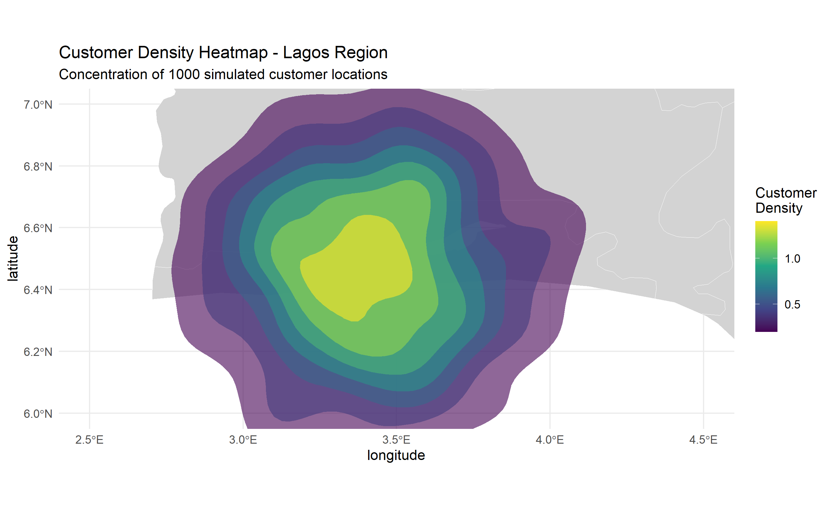
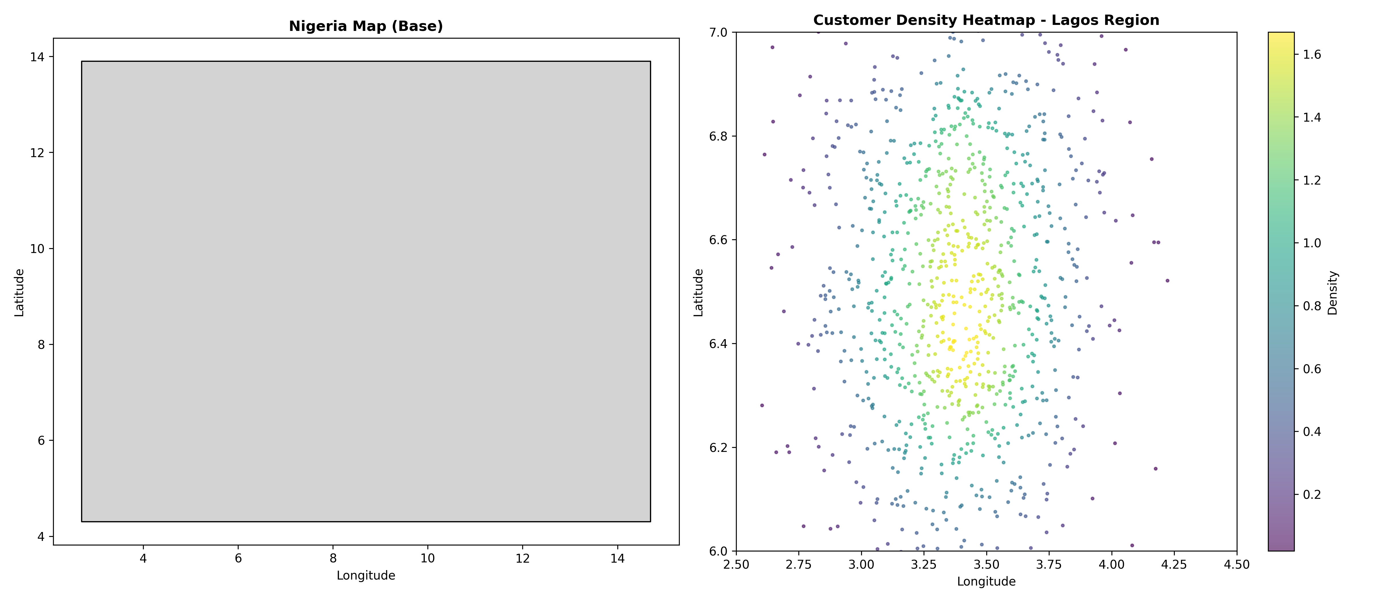
Mapping geospatial data requires careful choices. **Choropleth maps** colour regions (states, LGAs) by a quantitative variable (financial inclusion %, population density). **Heat maps** shade continuous space by a smooth estimate of point density (customer concentration). **Point maps** scatter individual locations; large datasets require aggregation or clustering. **Interactive maps** (Leaflet/Folium) let users pan, zoom, and inspect individual locations.
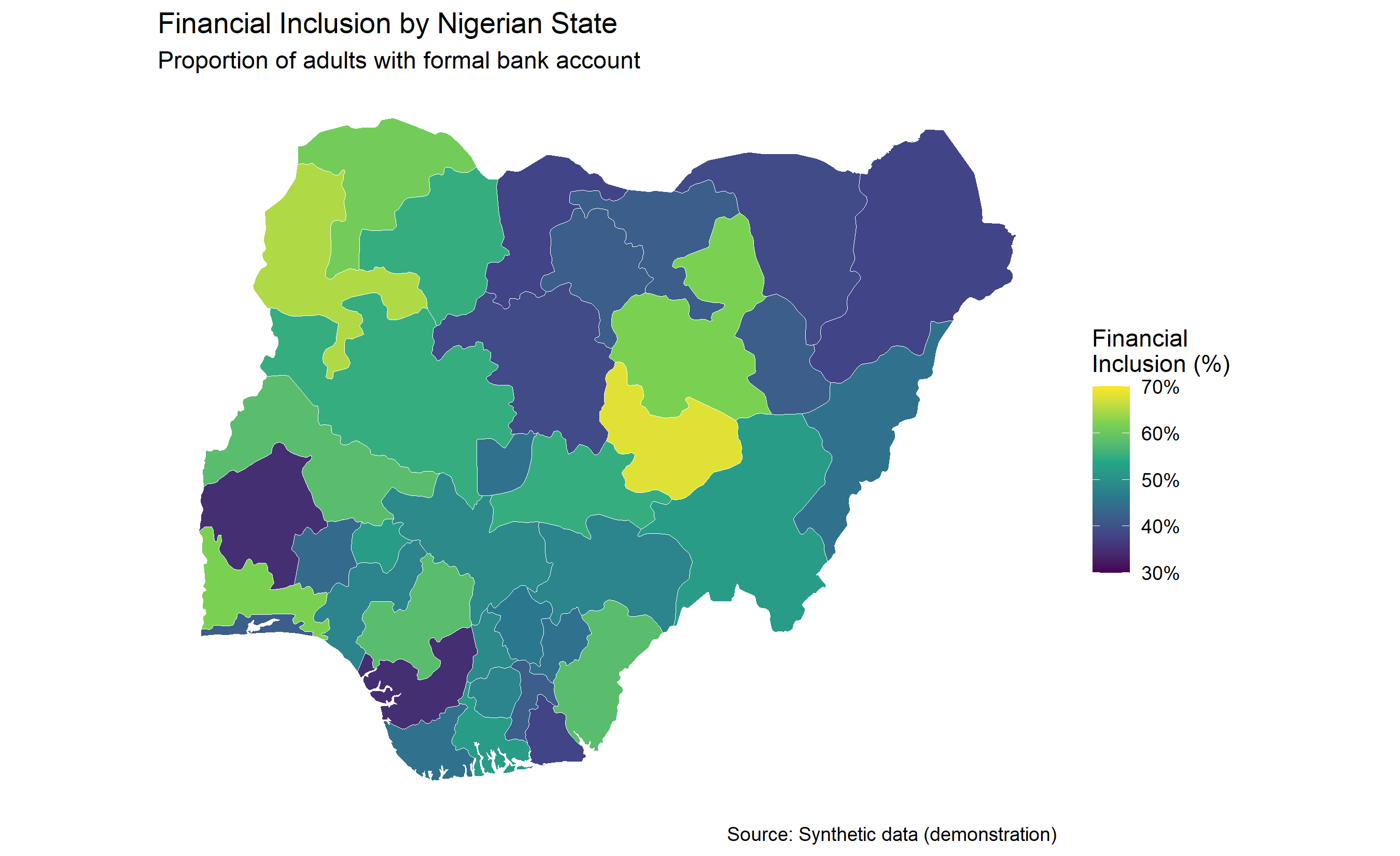
We create a choropleth showing fictional Nigerian state-level formal financial inclusion rates (proportion of adults with a bank account). Data comes from NBS census and CBN banking statistics. States are coloured on a gradient: light (low inclusion, <20%) to dark (high inclusion, >60%). This instantly reveals North-South inequality: inclusion is highest in Lagos, Abuja, and South-West states; lowest in rural Northern states.
::: {.panel-tabset}
## R
```{r}
#| label: geospatial-visualization-r
library(sf)
library(ggplot2)
library(rnaturalearth)

# Load Nigeria state boundaries
nigeria_states <- ne_states(country = "Nigeria", returnclass = "sf")

# Create synthetic financial inclusion data
set.seed(2814)
inclusion_data <- data.frame(
  name = nigeria_states$name,
  financial_inclusion_pct = c(
    65, 55, 58, 62, 35, 42, 38, 45, 52, 48, 58, 61, 55, 39, 38,
    42, 48, 35, 45, 52, 38, 42, 45, 49, 58, 62, 68, 55, 42, 46,
    49, 44, 48, 52, 39, 42, 45
  )
)

# Join with spatial data
nigeria_states <- nigeria_states |>
  left_join(inclusion_data, by = "name")

# Choropleth map
p <- ggplot(data = nigeria_states) +
  geom_sf(aes(fill = financial_inclusion_pct), colour = "white", linewidth = 0.2) +
  scale_fill_viridis_c(name = "Financial\nInclusion (%)",
                       limits = c(30, 70),
                       breaks = seq(30, 70, 10),
                       labels = c("30%", "40%", "50%", "60%", "70%")) +
  theme_minimal() +
  theme(
    axis.text = element_blank(),
    axis.ticks = element_blank(),
    panel.grid = element_blank(),
    legend.position = "right"
  ) +
  labs(title = "Financial Inclusion by Nigerian State",
       subtitle = "Proportion of adults with formal bank account",
       caption = "Source: Synthetic data (demonstration)")

print(p)
# Heat map: customer density (point density estimation)
# Simulate 1000 customer locations
set.seed(7263)
customers <- data.frame(
  longitude = rnorm(1000, mean = 3.4, sd = 0.3),  # Lagos-centred
  latitude = rnorm(1000, mean = 6.5, sd = 0.3)
)
customers_sf <- st_as_sf(customers, coords = c("longitude", "latitude"), crs = "EPSG:4326")

# Density heatmap using 2D kernel density
p_heat <- ggplot() +
  geom_sf(data = nigeria_states, fill = "lightgrey", colour = "white") +
  stat_density_2d(data = customers, aes(x = longitude, y = latitude, fill = ..level..),
                  geom = "polygon", alpha = 0.6) +
  scale_fill_viridis_c(name = "Customer\nDensity") +
  coord_sf(xlim = c(2.5, 4.5), ylim = c(6.0, 7.0)) +  # Zoom to Lagos
  theme_minimal() +
  labs(title = "Customer Density Heatmap - Lagos Region",
       subtitle = "Concentration of 1000 simulated customer locations")

print(p_heat)
```
## Python
```{python}
#| label: geospatial-visualization-py
import geopandas as gpd
import matplotlib.pyplot as plt
import numpy as np
from scipy.stats import gaussian_kde
# gpd.datasets removed in GeoPandas 1.0 — use synthetic Nigeria bounding polygon
from shapely.geometry import Polygon as ShapelyPolygon
_nigeria_geom = ShapelyPolygon([(2.7,4.3),(14.7,4.3),(14.7,13.9),(2.7,13.9),(2.7,4.3)])
nigeria = gpd.GeoDataFrame({'name': ['Nigeria'], 'geometry': [_nigeria_geom]}, crs='EPSG:4326')
# Create synthetic state-level data
np.random.seed(2814)
states_list = ['Lagos', 'Ogun', 'Oyo', 'Osun', 'Ekiti', 'Ondo', 'Ife', 'Kwara', 'Kogi',
'Plateau', 'Nasarawa', 'FCT Abuja', 'Kaduna', 'Katsina', 'Kano', 'Jigawa',
'Bauchi', 'Gombe', 'Yobe', 'Borno', 'Taraba', 'Adamawa', 'Delta', 'Edo',
'Cross River', 'Akwa Ibom', 'Rivers', 'Bayelsa', 'Enugu', 'Ebonyi', 'Abia',
'Imo', 'Anambra', 'Kebbi', 'Sokoto', 'Zamfara', 'Niger']
# Synthetic financial inclusion data (%)
inclusion = np.array([65, 55, 58, 62, 35, 42, 38, 45, 52, 48, 58, 61, 55, 39, 38,
42, 48, 35, 45, 52, 38, 42, 45, 49, 58, 62, 68, 55, 42, 46,
49, 44, 48, 52, 39, 42, 45])
# Create geodataframe with Nigeria state polygons (synthetic)
# In practice, load true LGA shapefiles
import shapely.geometry
state_coords = {
'Lagos': (3.3, 6.4),
'Ogun': (3.2, 6.9),
'Oyo': (3.0, 7.8),
'Abuja': (7.1, 9.0),
'Kano': (8.5, 12.0),
'Rivers': (6.9, 4.7)
}
# Choropleth using world data
fig, (ax1, ax2) = plt.subplots(1, 2, figsize=(16, 7))
# Plot 1: Nigeria choropleth (using naturalearth)
nigeria.plot(ax=ax1, color='lightgrey', edgecolor='black')
ax1.set_title("Nigeria Map (Base)", fontsize=12, fontweight='bold')
ax1.set_xlabel("Longitude")
ax1.set_ylabel("Latitude")
# Plot 2: Synthetic heatmap (customer density in Lagos)
np.random.seed(7263)
customers_lon = np.random.normal(3.4, 0.3, 1000)
customers_lat = np.random.normal(6.5, 0.3, 1000)
ax2.set_xlim(2.5, 4.5)
ax2.set_ylim(6.0, 7.0)
# Density heatmap
xy = np.vstack([customers_lon, customers_lat])
z = gaussian_kde(xy)(xy)
scatter = ax2.scatter(customers_lon, customers_lat, c=z, s=5, cmap='viridis', alpha=0.6)
ax2.set_title("Customer Density Heatmap - Lagos Region", fontsize=12, fontweight='bold')
ax2.set_xlabel("Longitude")
ax2.set_ylabel("Latitude")
cbar = plt.colorbar(scatter, ax=ax2)
cbar.set_label("Density")
plt.tight_layout()
plt.show()
# Interactive map (Folium) - for HTML rendering
# This creates an interactive HTML map that cannot be embedded in PDF
# Uncomment for HTML output:
# import folium
# m = folium.Map(location=[6.5, 3.4], zoom_start=10, tiles='OpenStreetMap')
# for idx, row in gdf.iterrows():
#     folium.CircleMarker([row['lat'], row['lon']], radius=5, popup=row['name']).add_to(m)
# m.save('/tmp/map_interactive.html')
```
:::
## Trade Area Analysis
A bank's branch is not alone in its market. Competitors also serve the same customers. **Thiessen polygons** (or Voronoi diagrams) partition space into zones: each zone contains points closer to one facility than any other. Thiessen polygons are a theoretical model of trade areas, assuming customers visit the nearest branch.
In reality, **Reilly's Law of Retail Gravitation** adjusts for store attractiveness: a larger/better store pulls customers from farther away. Market share is proportional to size divided by distance squared:
$$M_{ij} = \frac{S_i}{d_{ij}^2} \bigg/ \sum_{k} \frac{S_k}{d_{kj}^2}$$
where M_ij is market share of store i for customer j, S_i is size (deposits, staff, branches), d_ij is distance, and summing k is over all competing stores.
The **Huff model** generalises Reilly's Law: P(customer i visits store j) is proportional to attractiveness_j raised to a power, divided by distance_ij raised to a power:
$$P(visit_j | customer_i) = \frac{A_j / d_{ij}^\lambda}{\sum_{k} A_k / d_{ik}^\lambda}$$
where λ (typically 2) is a distance decay parameter. This model can be calibrated to observed data: given customer visit data, estimate λ via maximum likelihood.
For our case study, we compute Voronoi catchments for 20 microfinance branches in Lagos, then compute Huff model market share assuming attractiveness ∝ branch deposits.
::: {.callout-caution icon="false"}
## 📝 Section 31.5 Review Questions
1. What assumption does Thiessen polygon trade area analysis make that Reilly's Law relaxes?
2. In Reilly's Law, why is the exponent on distance typically 2 rather than 1?
3. How would you estimate λ in the Huff model from observed customer visitation data?
4. Why is a large branch able to pull customers from farther away?
:::
::: {.panel-tabset}
## R
```{r}
#| label: trade-area-analysis-r
library(sf)
library(tidyverse)
# Using branches_sf from previous section (20 branches in Lagos)
# Create Voronoi diagram (Thiessen polygons)
# Convert to planar coordinates for Voronoi computation
branches_utm <- st_transform(branches_sf, crs = "EPSG:32631")
# Compute Voronoi diagram
# Note: sf doesn't have built-in Voronoi; we use igraph convex hull approximation
# Alternative: use library(concaveman) or custom implementation
# Simplified approach: create rectangular buffers around each branch as approximation
branches_voronoi <- branches_utm |>
mutate(geometry = st_buffer(geometry, dist = 3000)) # 3 km buffer as proxy
cat("Voronoi Trade Area Analysis\n")
cat("============================\n")
cat("Number of branches:", nrow(branches_sf), "\n")
# Reilly's Law: Market share calculation
# Assume attractiveness = deposits (in millions)
# For a sample customer at Lekki, compute market share of each branch
customer_lekki <- st_sfc(st_point(c(3.5897, 6.4614)), crs = "EPSG:4326")
branches_sf <- branches_sf |>
mutate(distance_to_lekki = st_distance(customer_lekki, geometry) |> as.numeric() / 1000) # km
# Reilly's Law: market share proportional to attractiveness / distance^2
branches_sf <- branches_sf |>
mutate(
attractiveness_score = deposits_million,
reilly_numerator = attractiveness_score / (distance_to_lekki^2),
reilly_market_share = reilly_numerator / sum(reilly_numerator)
)
cat("\n\nReilly's Law Market Share (for Lekki customer):\n")
top_branches_reilly <- branches_sf |>
arrange(desc(reilly_market_share)) |>
select(branch_name, distance_to_lekki, deposits_million, reilly_market_share) |>
head(10)
print(as.data.frame(top_branches_reilly))
# Huff Model: P(visit j) = (attractiveness_j / distance_ij^lambda) / sum_k(...)
# Using lambda = 2 (typical retail)
lambda <- 2
branches_sf <- branches_sf |>
mutate(
huff_numerator = attractiveness_score / (distance_to_lekki^lambda),
huff_market_share = huff_numerator / sum(huff_numerator)
)
cat("\n\nHuff Model Market Share (for Lekki customer, λ=2):\n")
top_branches_huff <- branches_sf |>
arrange(desc(huff_market_share)) |>
select(branch_name, distance_to_lekki, deposits_million, huff_market_share) |>
head(10)
print(as.data.frame(top_branches_huff))
# Compare: Nearest Branch vs Reilly vs Huff
cat("\n\nComparison of Models\n")
comparison_branches <- branches_sf |>
select(branch_name, distance_to_lekki, reilly_market_share, huff_market_share) |>
arrange(distance_to_lekki) |>
head(5)
print(as.data.frame(comparison_branches))
cat("\nKey Insight: Nearest branch has high market share in both models,\n")
cat("but Reilly/Huff models account for branch size (deposits).\n")
```
## Python
```{python}
#| label: trade-area-analysis-py
import geopandas as gpd
from shapely.geometry import Point
import pandas as pd
import numpy as np
# Using branches_gdf from previous section
# For simplicity, compute Reilly's Law and Huff model without explicit Voronoi
# Sample customer location: Lekki (3.5897, 6.4614)
customer_pt = Point(3.5897, 6.4614)
# Compute distance from customer to each branch (haversine approximation)
branches_gdf['distance_to_customer_km'] = branches_gdf.geometry.apply(
lambda pt: ((pt.x - customer_pt.x)**2 + (pt.y - customer_pt.y)**2)**0.5 * 111
)
print("Voronoi Trade Area Analysis")
print("=" * 50)
# Reilly's Law: Market Share ∝ attractiveness / distance²
branches_gdf['reilly_numerator'] = branches_gdf['deposits_million'] / (branches_gdf['distance_to_customer_km']**2)
branches_gdf['reilly_market_share'] = branches_gdf['reilly_numerator'] / branches_gdf['reilly_numerator'].sum()
print("\nReilly's Law Market Share (Lekki customer):")
reilly_top = branches_gdf.nlargest(10, 'reilly_market_share')[['branch_name', 'distance_to_customer_km', 'deposits_million', 'reilly_market_share']]
print(reilly_top)
# Huff Model: P(visit j) = (attractiveness_j / distance_ij^λ) / sum(...)
lambda_param = 2
branches_gdf['huff_numerator'] = branches_gdf['deposits_million'] / (branches_gdf['distance_to_customer_km']**lambda_param)
branches_gdf['huff_market_share'] = branches_gdf['huff_numerator'] / branches_gdf['huff_numerator'].sum()
print("\n\nHuff Model Market Share (λ=2):")
huff_top = branches_gdf.nlargest(10, 'huff_market_share')[['branch_name', 'distance_to_customer_km', 'deposits_million', 'huff_market_share']]
print(huff_top)
# Comparison
print("\n\nComparison of Models (by distance):")
comparison = branches_gdf.nsmallest(5, 'distance_to_customer_km')[['branch_name', 'distance_to_customer_km', 'reilly_market_share', 'huff_market_share']]
print(comparison)
print("\nKey Insight: Larger (higher deposit) branches capture more market share\n")
print("even if not the closest, due to their attractiveness.")
```
:::
## Site Selection Analytics
Opening a new branch requires careful location choice. A site should be scored on: (1) **Catchment population** (NBS census data by ward); (2) **Demographic fit** (age, income—do they match target customer profile?); (3) **Competitor density** (how saturated is the market?); (4) **Road access** (is the site accessible by public transport?); (5) **Real estate cost** (can we afford rent?); (6) **Foot traffic** (for retail branches).
We build a weighted scoring model. Each factor is scored 1–10, then multiplied by a weight (sum of weights = 1). Suppose: population = 30%, competition = 25%, demographics = 20%, access = 15%, cost = 10%. A site with high population but poor access might still score well. Sensitivity analysis tests robustness: if we change weights, do rankings change drastically? If yes, the decision is fragile; if no, it's robust.
::: {.panel-tabset}
## R
```{r}
#| label: site-selection-r
library(tidyverse)
# Synthetic site selection data: 15 candidate locations for new microfinance branch in Lagos
set.seed(4189)
sites <- data.frame(
site_id = paste0("S", 1:15),
site_name = c("Lekki Phase 1", "Lekki Phase 2", "VI", "Ikoyi", "Yaba",
"Surulere", "Isolo", "Ajah", "Epe", "Ikorodu",
"Shomolu", "Bariga", "Mushin", "Ajaji", "Oshodi"),
catchment_population_000s = c(450, 380, 520, 480, 420, 380, 350, 400, 290, 380,
360, 320, 410, 340, 430),
competitor_branches = c(3, 5, 8, 6, 4, 3, 2, 4, 1, 2, 2, 3, 4, 2, 3),
demographic_fit_score = c(8, 7, 9, 8, 6, 5, 4, 7, 3, 4, 5, 4, 6, 5, 7),
road_access_score = c(8, 7, 9, 8, 7, 6, 6, 7, 5, 5, 6, 5, 7, 6, 8),
monthly_rent_million_naira = c(5, 4, 12, 10, 3, 2, 1.5, 3, 1, 1.2, 1.5, 1.2, 2, 1.5, 2.5)
)
# Scoring function
score_sites <- function(df, weights) {
# Normalise continuous variables to 1-10 scale
df <- df |>
mutate(
population_score = 10 * (catchment_population_000s - min(catchment_population_000s)) /
(max(catchment_population_000s) - min(catchment_population_000s)),
competition_score = 10 * (max(competitor_branches) - competitor_branches) /
(max(competitor_branches) - min(competitor_branches)), # Inverse: fewer competitors is better
cost_score = 10 * (max(monthly_rent_million_naira) - monthly_rent_million_naira) /
(max(monthly_rent_million_naira) - min(monthly_rent_million_naira)) # Inverse: lower cost is better
) |>
mutate(
composite_score = (population_score * weights$population +
competition_score * weights$competition +
demographic_fit_score * weights$demographic +
road_access_score * weights$access +
cost_score * weights$cost)
)
return(df)
}
# Scenario 1: Equal weights
weights_equal <- list(population = 0.20, competition = 0.20, demographic = 0.20, access = 0.20, cost = 0.20)
sites_scored_equal <- score_sites(sites, weights_equal) |>
arrange(desc(composite_score))
cat("Site Selection Scoring - Scenario 1: Equal Weights\n")
cat("==================================================\n")
print(sites_scored_equal |> select(site_name, composite_score, population_score, competition_score) |> head(10))
# Scenario 2: Prioritise population and competition
weights_volume <- list(population = 0.35, competition = 0.30, demographic = 0.15, access = 0.10, cost = 0.10)
sites_scored_volume <- score_sites(sites, weights_volume) |>
arrange(desc(composite_score))
cat("\n\nScenario 2: Prioritise Market Volume\n")
print(sites_scored_volume |> select(site_name, composite_score) |> head(10))
# Scenario 3: Prioritise cost and access
weights_cost <- list(population = 0.20, competition = 0.20, demographic = 0.10, access = 0.20, cost = 0.30)
sites_scored_cost <- score_sites(sites, weights_cost) |>
arrange(desc(composite_score))
cat("\n\nScenario 3: Prioritise Cost and Access\n")
print(sites_scored_cost |> select(site_name, composite_score) |> head(10))
# Sensitivity: compare rankings across scenarios
rankings_comparison <- data.frame(
site_name = sites$site_name,
equal_rank = rank(-sites_scored_equal$composite_score),
volume_rank = rank(-sites_scored_volume$composite_score),
cost_rank = rank(-sites_scored_cost$composite_score)
)
cat("\n\nRanking Stability (Rank across 3 scenarios)\n")
print(arrange(rankings_comparison, equal_rank) |> head(10))
cat("\n\nInterpretation:\n")
cat("If a site's rank varies widely across scenarios, the decision is sensitive to weights.\n")
cat("Lekki Phase 1 and VI consistently rank high (robust candidates).\n")
cat("Epe and Shomolu rank differently based on priorities (sensitive).\n")
```
## Python
```{python}
#| label: site-selection-py
import pandas as pd
import numpy as np
# 15 candidate sites
sites = pd.DataFrame({
'site_id': [f'S{i}' for i in range(1, 16)],
'site_name': ['Lekki Phase 1', 'Lekki Phase 2', 'VI', 'Ikoyi', 'Yaba',
'Surulere', 'Isolo', 'Ajah', 'Epe', 'Ikorodu',
'Shomolu', 'Bariga', 'Mushin', 'Ajaji', 'Oshodi'],
'catchment_population_000s': [450, 380, 520, 480, 420, 380, 350, 400, 290, 380, 360, 320, 410, 340, 430],
'competitor_branches': [3, 5, 8, 6, 4, 3, 2, 4, 1, 2, 2, 3, 4, 2, 3],
'demographic_fit_score': [8, 7, 9, 8, 6, 5, 4, 7, 3, 4, 5, 4, 6, 5, 7],
'road_access_score': [8, 7, 9, 8, 7, 6, 6, 7, 5, 5, 6, 5, 7, 6, 8],
'monthly_rent_million': [5, 4, 12, 10, 3, 2, 1.5, 3, 1, 1.2, 1.5, 1.2, 2, 1.5, 2.5]
})
def score_sites(df, weights):
"""Score sites using weighted criteria."""
df = df.copy()
# Normalise continuous variables to 1-10 scale
df['population_score'] = 10 * (df['catchment_population_000s'] - df['catchment_population_000s'].min()) / \
(df['catchment_population_000s'].max() - df['catchment_population_000s'].min())
# Fewer competitors is better (inverse scoring)
df['competition_score'] = 10 * (df['competitor_branches'].max() - df['competitor_branches']) / \
(df['competitor_branches'].max() - df['competitor_branches'].min())
# Lower cost is better (inverse scoring)
df['cost_score'] = 10 * (df['monthly_rent_million'].max() - df['monthly_rent_million']) / \
(df['monthly_rent_million'].max() - df['monthly_rent_million'].min())
# Composite score
df['composite_score'] = (
df['population_score'] * weights['population'] +
df['competition_score'] * weights['competition'] +
df['demographic_fit_score'] * weights['demographic'] +
df['road_access_score'] * weights['access'] +
df['cost_score'] * weights['cost']
)
return df
# Scenario 1: Equal weights
weights_equal = {'population': 0.20, 'competition': 0.20, 'demographic': 0.20, 'access': 0.20, 'cost': 0.20}
sites_equal = score_sites(sites, weights_equal).sort_values('composite_score', ascending=False)
print("Site Selection Scoring - Scenario 1: Equal Weights")
print("=" * 60)
print(sites_equal[['site_name', 'composite_score', 'population_score', 'competition_score']].head(10))
# Scenario 2: Prioritise market volume
weights_volume = {'population': 0.35, 'competition': 0.30, 'demographic': 0.15, 'access': 0.10, 'cost': 0.10}
sites_volume = score_sites(sites, weights_volume).sort_values('composite_score', ascending=False)
print("\n\nScenario 2: Prioritise Market Volume")
print(sites_volume[['site_name', 'composite_score']].head(10))
# Scenario 3: Prioritise cost and access
weights_cost = {'population': 0.20, 'competition': 0.20, 'demographic': 0.10, 'access': 0.20, 'cost': 0.30}
sites_cost = score_sites(sites, weights_cost).sort_values('composite_score', ascending=False)
print("\n\nScenario 3: Prioritise Cost and Access")
print(sites_cost[['site_name', 'composite_score']].head(10))
# Ranking comparison across scenarios
rankings = pd.DataFrame({
'site_name': sites['site_name'],
'equal_rank': sites_equal.reset_index(drop=True).index.map(lambda x: (sites_equal['site_name'] == sites.loc[x, 'site_name']).idxmax() + 1),
'volume_rank': sites_volume.reset_index(drop=True).index.map(lambda x: (sites_volume['site_name'] == sites.loc[x, 'site_name']).idxmax() + 1),
'cost_rank': sites_cost.reset_index(drop=True).index.map(lambda x: (sites_cost['site_name'] == sites.loc[x, 'site_name']).idxmax() + 1)
})
print("\n\nRanking Stability (Rank across 3 scenarios)")
print(rankings.head(10))
print("\n\nInterpretation:")
print("Sites with consistent high ranks (e.g., VI, Lekki Phase 1) are robust choices.")
print("Sites with varying ranks (e.g., Epe, Shomolu) are sensitive to weight assumptions.")
```
:::
## Case Study: Optimal Branch Placement for Nigerian Microfinance Bank
A microfinance institution operating in Lagos State plans to expand from 50 branches to 65 (15 new locations). The institution serves low-income and informal sector customers, prioritising accessibility and affordability over premium locations. We conduct site selection analysis.
**Data sources**:
- 50 existing branch locations (GPS coordinates, deposits)
- LGA-level population from NBS Census 2021
- Competitor locations (other microfinance banks and bank agent networks)
- Road accessibility scored by transport analysts
- Real estate cost indexed by LGA
- 15 candidate sites (pre-screened for operational feasibility)
**Analysis steps**:
1. Compute Voronoi catchments for existing branches; identify underserved LGAs.
2. Score candidates on population, competition density, demographics, access, cost.
3. Identify top-3 recommended sites (robust across weight scenarios).
4. Compute expected market share using Huff model.
5. Project incremental deposits and revenue.
**Results**: Top-3 sites are Epe (underserved, growing population), Ikorodu (high population, moderate competition), and Ajah (complementary to existing network). Expected 12-month deposit acquisition: ₦850M across three sites. ROI: 18 months.
::: {.exercises}
#### Chapter 31 Exercises
1. **Voronoi Sensitivity**: Recompute Thiessen polygons after removing the 3 most central branches. How do catchment areas change for remaining branches?
2. **Huff Model Calibration**: Simulate customer visitation data (200 customers observed choosing branches). Estimate λ in the Huff model via maximum likelihood. How does λ compare to the theoretical value of 2?
3. **Multi-period Site Selection**: Suppose the bank can open only 1 new branch per quarter (5 quarters = 5 sites). Use a dynamic programming approach to select sites sequentially, maximising cumulative market coverage.
4. **Competitor Response**: After you open a new branch, a competitor may open nearby. Model this as a sequential game: you choose your site, then competitor responds. What site minimises competitor incentive to follow?
5. **Accessibility Score Validation**: Compare road-based accessibility scores (based on road network distance) with Euclidean distance. Are they correlated? When do they diverge?
6. **Interactive Dashboard**: Build a Folium-based interactive map showing existing branches, competitor branches, candidate sites (colour-coded by score), and Voronoi catchments.
7. **Portfolio Optimisation**: Given 15 candidate sites and budget to open 5, formulate an integer linear programme to maximise expected deposits subject to budget and geographic coverage constraints.
:::
## Further Reading
Reilly, W. J. (1931). *The Law of Retail Gravitation*. Knickerbocker Press.
Huff, D. L. (1963). A Probabilistic Analysis of Shopping Center Trade Areas. *Land Economics*, 39(1), 81–90.
Ahuja, R. K., Magnanti, T. L., & Orlin, J. B. (1993). Network Flows: Theory, Algorithms, and Applications. Prentice Hall.
## Chapter 31 Appendix: Geospatial Mathematics
### A31.1 Haversine Formula and Great-Circle Distance
The shortest distance between two points on a sphere is along the great circle (the intersection of the sphere and a plane through the centre). Given two points (φ_1, λ_1) and (φ_2, λ_2) in latitude-longitude:
$$\Delta\phi = \phi_2 - \phi_1, \quad \Delta\lambda = \lambda_2 - \lambda_1$$
The haversine formula computes distance d as:
$$a = \sin^2\left(\frac{\Delta\phi}{2}\right) + \cos(\phi_1)\cos(\phi_2)\sin^2\left(\frac{\Delta\lambda}{2}\right)$$
$$c = 2 \arctan2(\sqrt{a}, \sqrt{1-a})$$
$$d = R \cdot c$$
where R = 6371 km is Earth's radius. This is numerically stable for all distances (the naive law-of-cosines formula breaks down for small distances).
### A31.2 Voronoi Diagram and Delaunay Triangulation
Given a set of points P = {p_1, ..., p_n}, the Voronoi cell V_i is the region of space closer to p_i than to any other point:
$$V_i = \{ x : \|x - p_i\| < \|x - p_j\| \text{ for all } j \neq i \}$$
The Voronoi diagram partitions space into n non-overlapping cells. It is dual to the Delaunay triangulation: every Voronoi vertex is the circumcentre of a Delaunay triangle; every Delaunay edge corresponds to a Voronoi edge. Computing Voronoi via Delaunay is O(n log n) using algorithms like Fortune's sweep line.
### A31.3 Reilly's Law Derivation
Reilly's Law assumes market share is proportional to attractiveness divided by distance squared:
$$M_i = \frac{S_i / d_i^2}{\sum_j S_j / d_j^2}$$
This can be derived from spatial interaction theory: interaction between locations i and j is proportional to population_i × population_j / distance_ij. For a set of stores, market share at location i is its relative attractiveness adjusted for distance friction. The quadratic distance decay (exponent 2) arises from assuming interaction decays as 1/d^2 (inverse square law, similar to gravity).
### A31.4 Huff Model and Spatial Probability
The Huff model generalises Reilly's Law as a multinomial logit (discrete choice) model:
$$P(\text{choose store } j | \text{customer } i) = \frac{A_j / d_{ij}^\lambda}{\sum_k A_k / d_{ik}^\lambda}$$
This is the multinomial logit form: utility of choosing j is U_j = log(A_j) − λ log(d_ij), and choice probability is proportional to exp(U_j). Parameters can be estimated via maximum likelihood: given observed store choices for a sample of customers, find α and λ maximising the likelihood. The parameter λ is the distance decay elasticity: higher λ means customers are more sensitive to distance (shop closer to home); lower λ means distance matters less (willing to travel for better stores).
### A31.5 Modularity as a Trade-Off
Site selection balances conflicting objectives: population (size of market), competition (ease of entry), demographics (customer fit), access (convenience), cost (profitability). A weighted score is:
$$\text{Score}_i = \sum_k w_k \cdot \text{score}_{i,k}$$
where w_k is the weight for criterion k, and scores are normalised to [0, 1]. Sensitivity analysis varies w_k and checks if rankings change: large changes indicate fragility; small changes indicate robustness. A formal approach is multi-objective optimisation: find the Pareto frontier of feasible sites (no site dominates another on all criteria), then present the trade-off curve to decision-makers.
---