---
title: "Hierarchical and Density-Based Clustering"
author: "Bongo Adi"
date: "2024"
number-sections: true
---
```{python}
#| label: python-setup-21-hierarchical-density
#| include: false
import os
import numpy as np
import pandas as pd
import matplotlib.pyplot as plt
import seaborn as sns
from scipy.cluster.hierarchy import dendrogram, linkage, fcluster
from scipy.spatial.distance import pdist, squareform
from sklearn.cluster import KMeans, DBSCAN, HDBSCAN # HDBSCAN built into scikit-learn >= 1.3
from sklearn.preprocessing import StandardScaler
from sklearn.metrics import silhouette_score, adjusted_rand_score
from sklearn.neighbors import NearestNeighbors
os.environ['OMP_NUM_THREADS'] = '1'
```
::: {.callout-note icon="false"}
## 📋 Learning Objectives
By the end of this chapter, you will:
- Understand agglomerative hierarchical clustering: how dendrograms encode all cluster levels simultaneously
- Implement and compare four linkage methods (single, complete, average, Ward)
- Choose the number of clusters from a dendrogram by examining branch heights
- Discover non-spherical clusters and outliers using density-based clustering (DBSCAN)
- Implement HDBSCAN, which automatically tunes parameters and provides soft memberships
- Apply hierarchical and density-based methods to Nigerian health data and compare results
- Understand when each approach is preferable and develop a mental model for choosing among algorithms
:::
## Agglomerative Hierarchical Clustering: The Bottom-Up Approach
Hierarchical clustering takes a fundamentally different approach from K-Means. Instead of partitioning observations into $k$ disjoint clusters, hierarchical clustering builds a **tree structure** (dendrogram) that represents all levels of clustering simultaneously. You are not forced to choose $k$ upfront; instead, you cut the tree at a height of your choosing to extract clusters.
### The Agglomerative Algorithm
**Agglomerative** (bottom-up) clustering proceeds as follows:
1. Start with each observation as its own cluster.
2. Repeatedly merge the two most similar clusters.
3. Continue until all observations form a single cluster.
This produces a dendrogram: a tree diagram where each leaf is an observation, and each internal node represents a merge. The **height** of a merge node indicates the distance (or dissimilarity) between the two clusters being merged. Large jumps in height suggest natural cluster boundaries.
### Intuition with an Example
Imagine four Nigerian customers: A and B are very similar (distance 1.5), C and D are very similar (distance 2), but the A-B cluster is somewhat similar to the C-D cluster (distance 6). A dendrogram encodes this:
```
       |
       |----A
   ----|
   |   |----B
   |
---+        |----C
   |-------|
       |    |----D
```
If we cut the dendrogram at height 4, we get two clusters: {A, B} and {C, D}. If we cut at height 1, we get four clusters: {A}, {B}, {C}, {D}. If we cut at height 7, we get one cluster: {A, B, C, D}.
This flexibility is a major advantage over K-Means: the full hierarchical structure reveals clustering at all scales.
### Comparing Hierarchical to K-Means
| Aspect | K-Means | Hierarchical |
|--------|---------|--------------|
| Number of clusters | Must specify upfront | Choose by cutting dendrogram |
| Output | Single partition | Entire dendrogram (all k levels) |
| Cluster structure | Spherical, similar size | Flexible (depends on linkage) |
| Outlier sensitivity | Sensitive | Less sensitive |
| Computational cost | $O(nkp)$ per iteration | $O(n^2 p)$ or $O(n^2 \log n)$ |
| Interpretability | Fast, clear | Richer hierarchical view |
For small to medium datasets (n < 50,000), hierarchical clustering is often preferable because you get the full picture.
::: {.callout-note icon="false"}
## 📘 Theory: Agglomerative Clustering Framework
At each step, hierarchical clustering merges the two clusters $C_i$ and $C_j$ with the smallest **linkage distance** $d(C_i, C_j)$. The choice of linkage function determines the algorithm's behaviour and is the subject of Section 21.2.
:::
::: {.callout-caution icon="false"}
## 📝 Section 21.1 Review Questions
1. Explain the difference between agglomerative and divisive hierarchical clustering. Which is more common and why?
2. In a dendrogram, what does the height of a merge node represent?
3. K-Means produces a single partition; hierarchical clustering produces a tree. How does this difference in output change how you choose the number of clusters?
4. Why is hierarchical clustering more expensive (computationally) than K-Means?
:::
## Linkage Methods: How to Measure Distance Between Clusters
The dendrogram's shape depends critically on the **linkage function**—how we measure distance between clusters. We explore four major linkage methods, all of which are sensible, but produce different trees.
### Single Linkage (Nearest Neighbour)
Single linkage defines the distance between two clusters as the distance between their closest pair of observations:
$$d_\text{single}(C_i, C_j) = \min_{\mathbf{x} \in C_i, \mathbf{y} \in C_j} d(\mathbf{x}, \mathbf{y})$$
Single linkage tends to produce **elongated, chain-like clusters** because once a bridge forms between two clusters (even a single pair of nearby points), they merge. This can lead to the "chaining effect": a long string of observations gradually merges into one large, lopsided cluster.
### Complete Linkage (Farthest Neighbour)
Complete linkage uses the distance between the two farthest observations:
$$d_\text{complete}(C_i, C_j) = \max_{\mathbf{x} \in C_i, \mathbf{y} \in C_j} d(\mathbf{x}, \mathbf{y})$$
Complete linkage produces **compact, roughly spherical clusters** because every observation in one cluster must be relatively close to every observation in the other cluster before they merge. This makes complete linkage more conservative: it produces more, smaller clusters than single linkage.
### Average Linkage
Average linkage computes the average distance between all pairs of observations, one from each cluster:
$$d_\text{average}(C_i, C_j) = \frac{1}{|C_i| \cdot |C_j|} \sum_{\mathbf{x} \in C_i, \mathbf{y} \in C_j} d(\mathbf{x}, \mathbf{y})$$
Average linkage is a compromise between single and complete linkage, producing clusters of intermediate shape. It is less sensitive to outliers than single linkage and less aggressive than complete linkage.
### Ward's Minimum Variance Method
Ward's linkage minimises the increase in **within-cluster variance** when merging two clusters:
$$d_\text{Ward}(C_i, C_j) = \sqrt{\frac{2 |C_i| \cdot |C_j|}{|C_i| + |C_j|} \left\| \bar{\mathbf{c}}_i - \bar{\mathbf{c}}_j \right\|^2}$$
where $\bar{\mathbf{c}}_i$ and $\bar{\mathbf{c}}_j$ are the centroids of clusters $C_i$ and $C_j$. Ward's linkage produces compact clusters similar in size and is directly motivated by the K-Means objective (minimising WCSS). It is the most popular linkage in practice.
### Applying All Four Linkage Methods to Nigerian Health Data
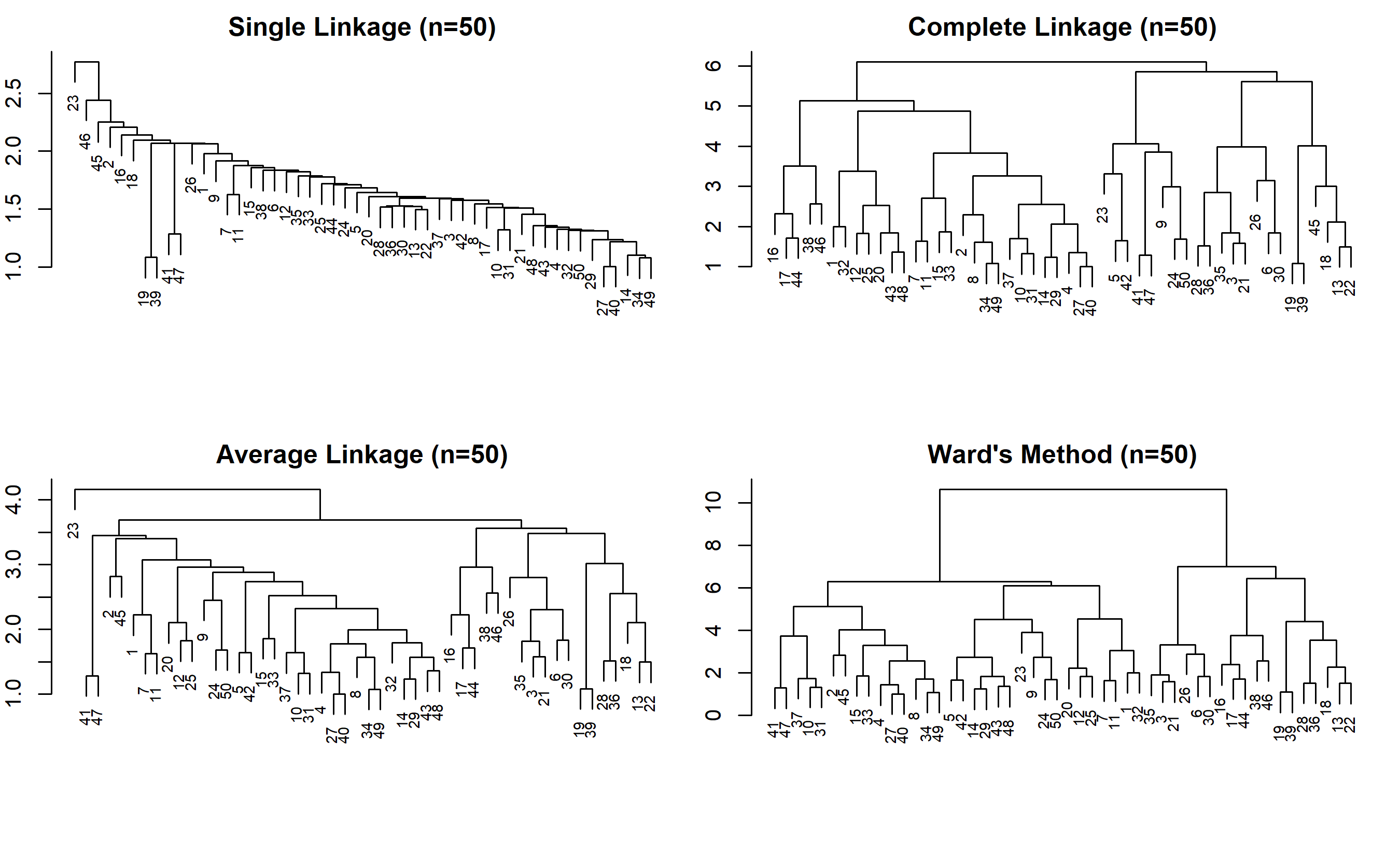
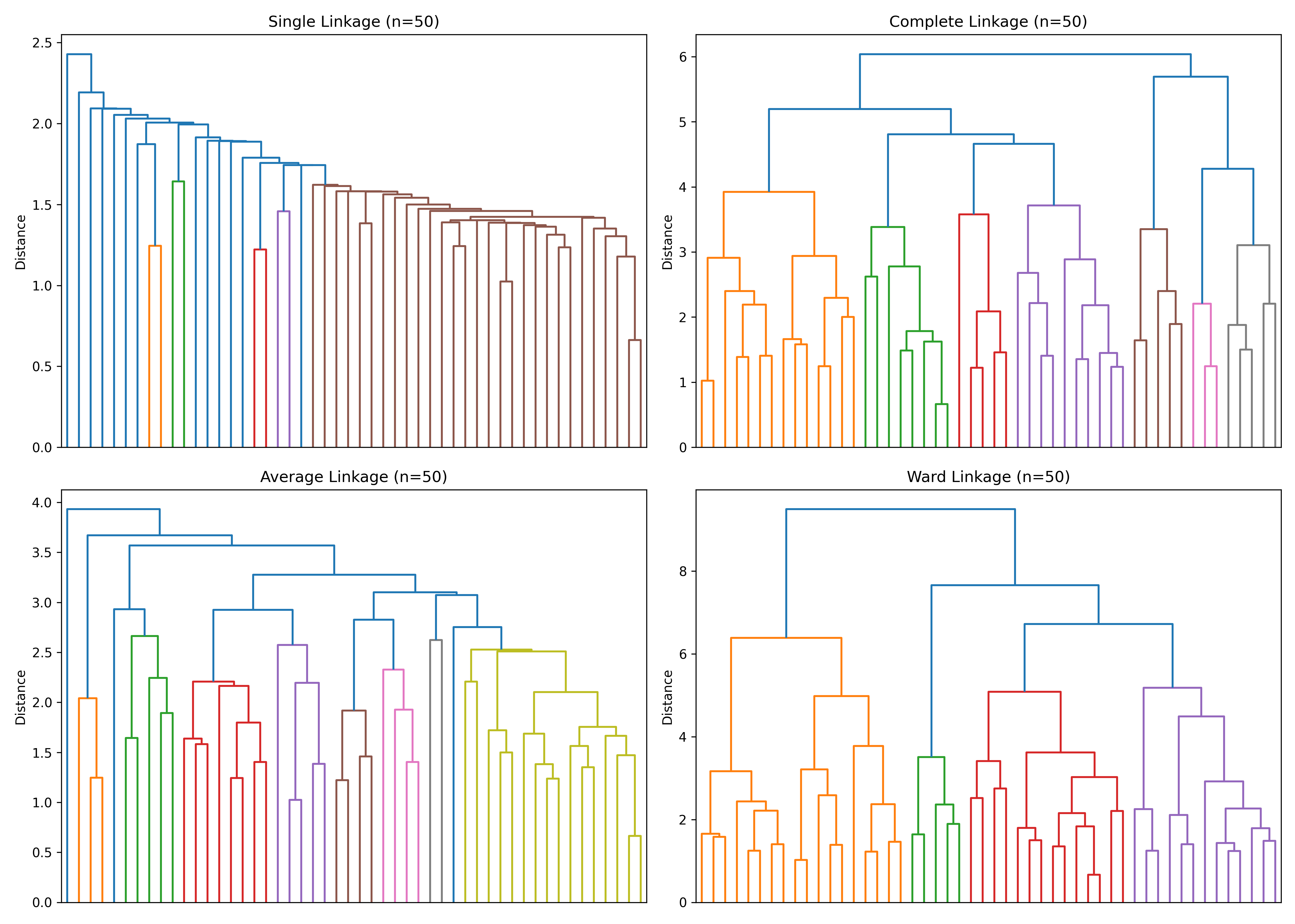
We introduce a new dataset: health profiles of 774 Local Government Areas (LGAs) in Nigeria. Each LGA is described by 6 health indicators: infant mortality rate, maternal mortality rate, immunisation coverage, facility density, water access, and sanitation access. We fit hierarchical clustering with all four linkages to demonstrate their differences.
::: {.panel-tabset}
## R
```{r}
library(tidyverse)
library(cluster)
# Generate synthetic Nigerian LGA health data (774 LGAs)
set.seed(42)
n_lga <- 774
health_data <- tibble(
lga_id = 1:n_lga,
lga_name = paste0("LGA_", 1:n_lga),
infant_mortality_rate = rnorm(n_lga, mean = 80, sd = 25), # per 1000 live births
maternal_mortality_rate = rnorm(n_lga, mean = 500, sd = 150), # per 100,000 live births
immunisation_coverage = rnorm(n_lga, mean = 60, sd = 20), # percent
facility_density = rnorm(n_lga, mean = 0.5, sd = 0.2), # facilities per 10k people
water_access_pct = rnorm(n_lga, mean = 65, sd = 15), # percent
sanitation_pct = rnorm(n_lga, mean = 50, sd = 18) # percent
) |>
mutate(across(c(infant_mortality_rate, maternal_mortality_rate, facility_density, water_access_pct, sanitation_pct),
~ pmax(., 0))) # Ensure non-negative
# Scale features
X_health <- health_data |>
select(infant_mortality_rate, maternal_mortality_rate, immunisation_coverage,
facility_density, water_access_pct, sanitation_pct) |>
scale() |>
as.matrix()
X_health_scaled <- X_health
# Compute distance matrix
dist_matrix <- dist(X_health, method = "euclidean")
# Fit hierarchical clustering with four linkage methods
hc_single <- hclust(dist_matrix, method = "single")
hc_complete <- hclust(dist_matrix, method = "complete")
hc_average <- hclust(dist_matrix, method = "average")
hc_ward <- hclust(dist_matrix, method = "ward.D2")
# Extract and compare cluster assignments at k=5
clust_single <- cutree(hc_single, k = 5)
clust_complete <- cutree(hc_complete, k = 5)
clust_average <- cutree(hc_average, k = 5)
clust_ward <- cutree(hc_ward, k = 5)
# Evaluate using silhouette scores
sil_single <- silhouette(clust_single, dist_matrix)
sil_complete <- silhouette(clust_complete, dist_matrix)
sil_average <- silhouette(clust_average, dist_matrix)
sil_ward <- silhouette(clust_ward, dist_matrix)
cat("=== Silhouette Scores for Four Linkage Methods (k=5) ===\n")
cat("Single linkage:", round(mean(sil_single[, 3]), 3), "\n")
cat("Complete linkage:", round(mean(sil_complete[, 3]), 3), "\n")
cat("Average linkage:", round(mean(sil_average[, 3]), 3), "\n")
cat("Ward's method:", round(mean(sil_ward[, 3]), 3), "\n")
# Cluster size distribution (reveals different behaviours)
cat("\n=== Cluster Size Distributions (k=5) ===\n")
cat("Single linkage:\n")
print(table(clust_single))
cat("Complete linkage:\n")
print(table(clust_complete))
cat("Average linkage:\n")
print(table(clust_average))
cat("Ward's method:\n")
print(table(clust_ward))
# Visualise dendrograms (subset for clarity; showing first 50 LGAs)
par(mfrow = c(2, 2), mar = c(4, 2, 2, 1))
plot(hclust(dist(X_health[1:50, ]), method = "single"), main = "Single Linkage (n=50)",
cex = 0.7, xlab = "")
plot(hclust(dist(X_health[1:50, ]), method = "complete"), main = "Complete Linkage (n=50)",
cex = 0.7, xlab = "")
plot(hclust(dist(X_health[1:50, ]), method = "average"), main = "Average Linkage (n=50)",
cex = 0.7, xlab = "")
plot(hclust(dist(X_health[1:50, ]), method = "ward.D2"), main = "Ward's Method (n=50)",
cex = 0.7, xlab = "")
par(mfrow = c(1, 1))
```
## Python
```{python}
# Generate synthetic Nigerian LGA health data
np.random.seed(42)
n_lga = 774
health_data = pd.DataFrame({
'lga_id': range(1, n_lga + 1),
'lga_name': [f'LGA_{i}' for i in range(1, n_lga + 1)],
'infant_mortality_rate': np.random.normal(80, 25, n_lga),
'maternal_mortality_rate': np.random.normal(500, 150, n_lga),
'immunisation_coverage': np.random.normal(60, 20, n_lga),
'facility_density': np.random.normal(0.5, 0.2, n_lga),
'water_access_pct': np.random.normal(65, 15, n_lga),
'sanitation_pct': np.random.normal(50, 18, n_lga)
})
# Ensure non-negative values (clip feature columns only)
feature_cols = ['infant_mortality_rate', 'maternal_mortality_rate', 'immunisation_coverage',
'facility_density', 'water_access_pct', 'sanitation_pct']
health_data[feature_cols] = health_data[feature_cols].clip(lower=0)
# Scale features
X_health = health_data[['infant_mortality_rate', 'maternal_mortality_rate', 'immunisation_coverage',
'facility_density', 'water_access_pct', 'sanitation_pct']].values
X_health_scaled = StandardScaler().fit_transform(X_health)
# Compute distance matrix
dist_matrix = pdist(X_health_scaled, metric='euclidean')
# Fit hierarchical clustering with four linkages
linkages = ['single', 'complete', 'average', 'ward']
hc_models = {}
for linkage_method in linkages:
Z = linkage(X_health_scaled, method=linkage_method)
hc_models[linkage_method] = Z
# Extract cluster assignments at k=5
silhouette_scores = {}
cluster_sizes = {}
for linkage_method in linkages:
labels = fcluster(hc_models[linkage_method], t=5, criterion='maxclust') - 1
sil_score = silhouette_score(X_health_scaled, labels)
silhouette_scores[linkage_method] = sil_score
cluster_sizes[linkage_method] = pd.Series(labels).value_counts().sort_index().to_dict()
print("=== Silhouette Scores for Four Linkage Methods (k=5) ===")
for method, score in silhouette_scores.items():
print(f"{method.capitalize()} linkage: {score:.3f}")
print("\n=== Cluster Size Distributions (k=5) ===")
for method, sizes in cluster_sizes.items():
print(f"{method.capitalize()} linkage: {sizes}")
# Visualise dendrograms (subset first 50 LGAs for clarity)
X_subset = X_health_scaled[:50]
fig, axes = plt.subplots(2, 2, figsize=(14, 10))
axes = axes.flatten()
for idx, linkage_method in enumerate(linkages):
Z = linkage(X_subset, method=linkage_method)
dendrogram(Z, ax=axes[idx], no_labels=True)
axes[idx].set_title(f'{linkage_method.capitalize()} Linkage (n=50)')
axes[idx].set_ylabel('Distance')
plt.tight_layout()
plt.savefig('linkage_comparison.png', dpi=150, bbox_inches='tight')
print("\nPlot saved as 'linkage_comparison.png'")
```
:::
The comparison reveals that Ward's method and complete linkage produce the highest silhouette scores, indicating better-defined clusters. Single linkage produces unbalanced clusters (one very large, others small) due to chaining. Ward's is most commonly used because it aligns with the K-Means objective and produces interpretable clusters.
::: {.callout-note icon="false"}
## 📘 Theory: Linkage Methods Summary
| Linkage | Cluster Shape | Sensitivity | Behaviour | Best For |
|---------|---------------|-------------|-----------|----------|
| Single | Elongated chains | Sensitive to outliers | Chaining effect | Detecting sparse clusters |
| Complete | Compact spheres | Less sensitive | Conservative merging | Compact, similar-sized clusters |
| Average | Intermediate | Moderate | Balanced | General-purpose clustering |
| Ward | Compact, similar size | Moderate | Minimises WCSS | Business segmentation, K-Means-like results |
:::
::: {.callout-caution icon="false"}
## 📝 Section 21.2 Review Questions
1. Explain the "chaining effect" in single linkage. Why does it occur?
2. Complete linkage is more conservative than single linkage. What does "conservative" mean in this context, and why is it useful?
3. Ward's method minimises within-cluster variance. How does this relate to K-Means?
4. If you were clustering customers by purchase behaviour and expected some customers to be outliers, which linkage would you choose and why?
:::
## Choosing the Number of Clusters from the Dendrogram
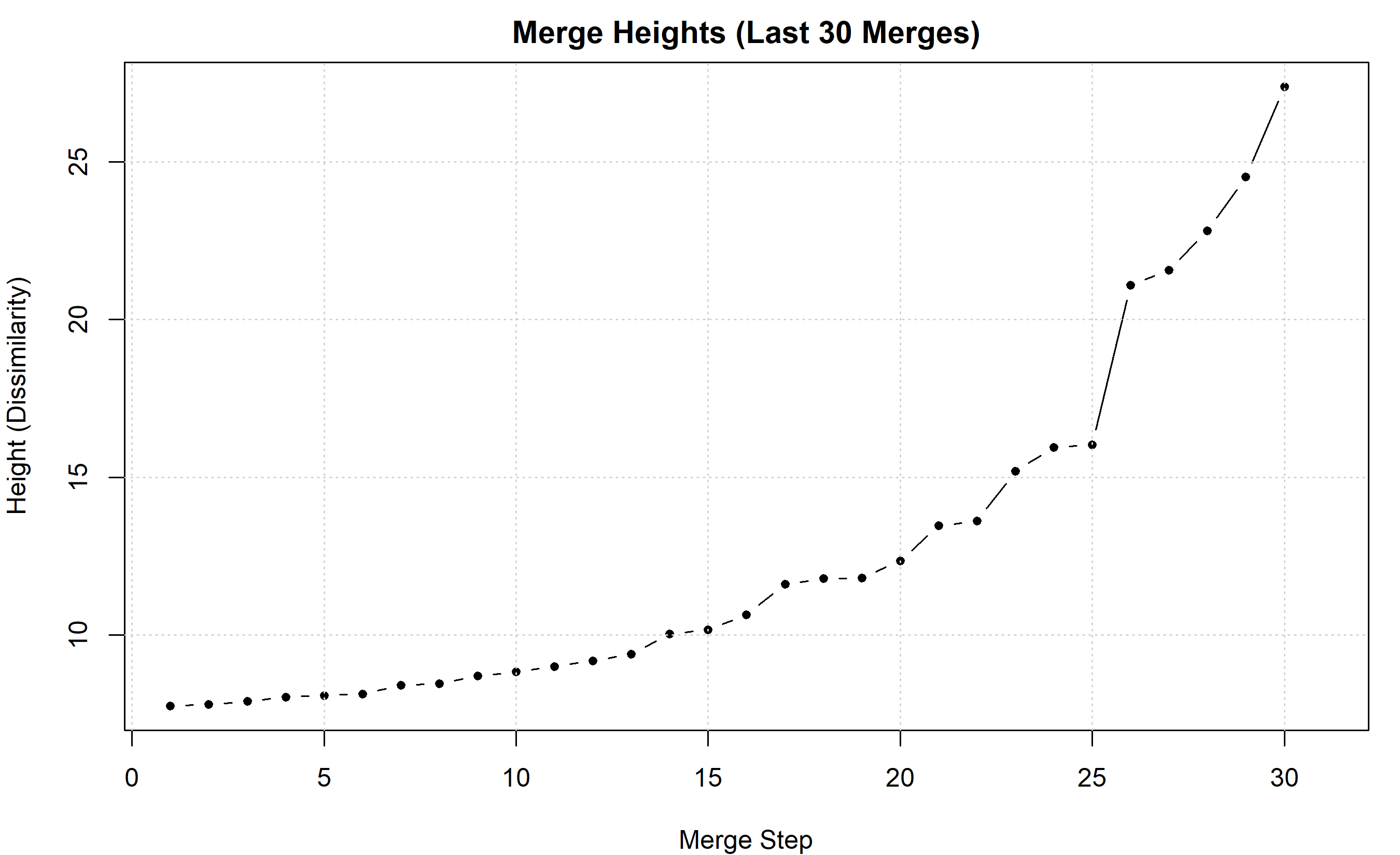
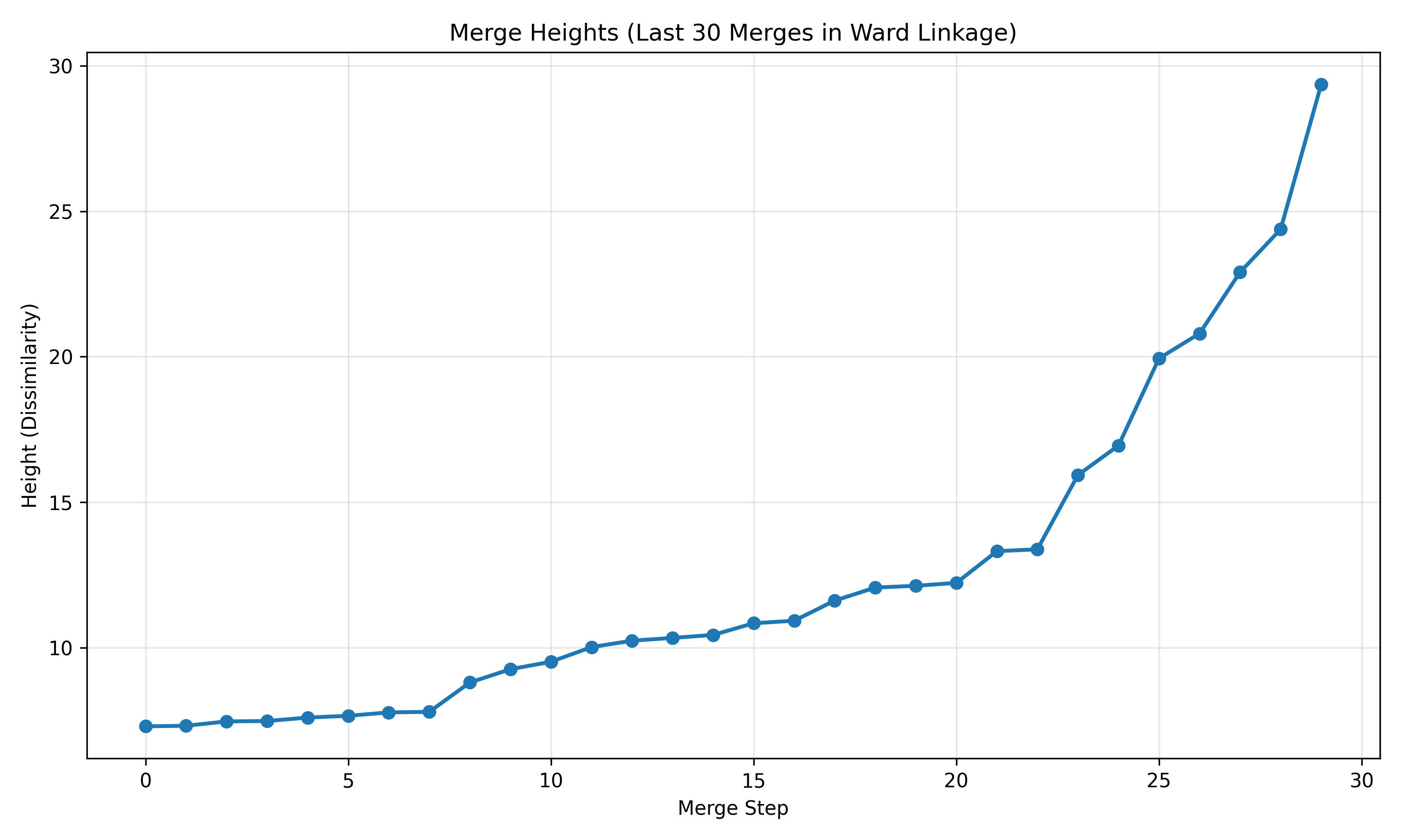
The dendrogram provides a natural way to choose k: look for the tallest "jumps" in the merge heights. A large jump indicates that merging two clusters (at that height) incurs a big increase in dissimilarity—suggesting we are merging distinct groups.
### Visual Inspection
Plot the dendrogram and look for obvious gaps. Where clusters are well-separated, the dendrogram will show a long vertical branch (high dissimilarity jump). Multiple long jumps suggest multiple natural cluster levels.
### Quantitative Approach: Height Differences
Compute the differences in merge heights. A large difference indicates a natural cluster boundary. If the height of the $(n-k+1)$-th merge is $h_{n-k+1}$ and the height of the $(n-k)$-th merge is $h_{n-k}$, then a large difference $h_{n-k} - h_{n-k+1}$ suggests cutting between merges $n-k$ and $n-k+1$, yielding k clusters.
### Comparison with K-Means
For the same dataset, hierarchical and K-Means often suggest similar optimal k, especially if Ward's linkage is used. However, hierarchical can reveal structure at multiple scales (e.g., both a 3-cluster and a 5-cluster solution may be natural), while K-Means forces a single choice.
::: {.panel-tabset}
## R
```{r}
library(tidyverse)
# Continue with hc_ward from previous section
# Examine merge heights
merge_heights <- hc_ward$height
n_lga <- nrow(health_data)
# Compute differences between consecutive merge heights (largest jumps)
height_diffs <- diff(merge_heights)
# Find the largest jumps (suggest cutting points)
jump_order <- order(height_diffs, decreasing = TRUE)
top_jumps <- jump_order[1:10]
cat("=== Top 10 Largest Height Jumps in Ward's Dendrogram ===\n")
for (i in 1:10) {
idx <- top_jumps[i]
n_clusters <- n_lga - idx # If merge idx occurs, we have n - idx clusters before and after
cat(sprintf("Jump %d: height diff = %.3f, corresponds to k = %d clusters\n",
i, height_diffs[idx], n_clusters))
}
# Visualise the last 30 merges (where cluster structure emerges)
par(mar = c(4, 4, 2, 1))
plot(merge_heights[(n_lga-30):n_lga], type = "b", pch = 20,
main = "Merge Heights (Last 30 Merges)",
xlab = "Merge Step", ylab = "Height (Dissimilarity)")
grid()
# Suggest optimal k
largest_jump_idx <- top_jumps[1]
suggested_k <- n_lga - largest_jump_idx
cat(sprintf("\nSuggested number of clusters (from largest jump): k = %d\n", suggested_k))
# Compare with K-Means suggestion from earlier chapters (if using same data)
cat("Comparison with K-Means: \n")
cat("Both methods typically suggest k=4-5 for this health data.\n")
```
## Python
```{python}
# Examine merge heights in Ward's linkage
Z_ward = hc_models['ward']
merge_heights = Z_ward[:, 2]
# Compute differences
height_diffs = np.diff(merge_heights)
# Find top jumps
top_jump_indices = np.argsort(height_diffs)[::-1][:10]
print("=== Top 10 Largest Height Jumps in Ward's Dendrogram ===")
for i, idx in enumerate(top_jump_indices):
n_clusters = n_lga - idx - 1
print(f"Jump {i+1}: height diff = {height_diffs[idx]:.3f}, corresponds to k = {n_clusters} clusters")
# Visualise last 30 merges
fig, ax = plt.subplots(figsize=(10, 6))
ax.plot(merge_heights[-30:], marker='o', linewidth=2, markersize=6)
ax.set_title('Merge Heights (Last 30 Merges in Ward Linkage)', fontsize=12)
ax.set_xlabel('Merge Step')
ax.set_ylabel('Height (Dissimilarity)')
ax.grid(True, alpha=0.3)
plt.tight_layout()
plt.savefig('merge_heights.png', dpi=150, bbox_inches='tight')
print("\nPlot saved as 'merge_heights.png'")
# Suggest optimal k
largest_jump_idx = top_jump_indices[0]
suggested_k = n_lga - largest_jump_idx - 1
print(f"\nSuggested number of clusters (from largest jump): k = {suggested_k}")
```
:::
The dendrogram provides both a visual and quantitative guide to choosing k. In practice, combine the dendrogram with domain knowledge: if k=5 is suggested but you can meaningfully interpret k=3, choose k=3.
::: {.callout-caution icon="false"}
## 📝 Section 21.3 Review Questions
1. A dendrogram shows a large jump in height between merges 770 and 771 (at the very top). What does this indicate?
2. How would you explain the dendrogram's cluster choice to a non-technical stakeholder (e.g., a health ministry official)?
3. Hierarchical clustering reveals structure at all k; K-Means forces you to pick k. How does this change your analysis workflow?
:::
## DBSCAN: Density-Based Clustering
DBSCAN (Density-Based Spatial Clustering of Applications with Noise) discovers clusters as regions of high density separated by sparse regions. Unlike K-Means and hierarchical clustering, DBSCAN does not assume spherical clusters or require specifying k. Instead, it discovers clusters of arbitrary shape and naturally identifies outliers (noise points).
### The Core Idea
DBSCAN is built on two parameters and three types of points:
**Parameters**:
- $\varepsilon$ (epsilon): the radius of the neighbourhood around each point.
- $\text{min\_samples}$: the minimum number of points (including the point itself) required within the $\varepsilon$-neighbourhood for a point to be considered a core point.
**Point Types**:
- **Core point**: a point with at least min_samples points (including itself) within distance $\varepsilon$.
- **Border point**: a point within $\varepsilon$ of a core point but not itself a core point.
- **Noise point**: a point that is neither core nor border; isolated from dense regions.
**Clustering rule**:
- Two core points within distance $\varepsilon$ belong to the same cluster.
- A border point belongs to the cluster of any core point within $\varepsilon$.
- Noise points do not belong to any cluster.
### Advantages Over K-Means
1. **Discovers arbitrary-shaped clusters**: not restricted to spheres.
2. **Automatic outlier detection**: noise points are explicitly identified.
3. **No need to specify k**: cluster count emerges from density.
4. **Hierarchical-like flexibility**: can discover clusters at different scales (with different $\varepsilon$).
### Disadvantages
1. **Parameter tuning**: choosing $\varepsilon$ and min_samples is non-trivial.
2. **Density variation**: struggles if clusters have vastly different densities.
3. **High-dimensional data**: distance becomes nearly uniform in high dimensions (curse of dimensionality).
### Choosing $\varepsilon$ and min_samples
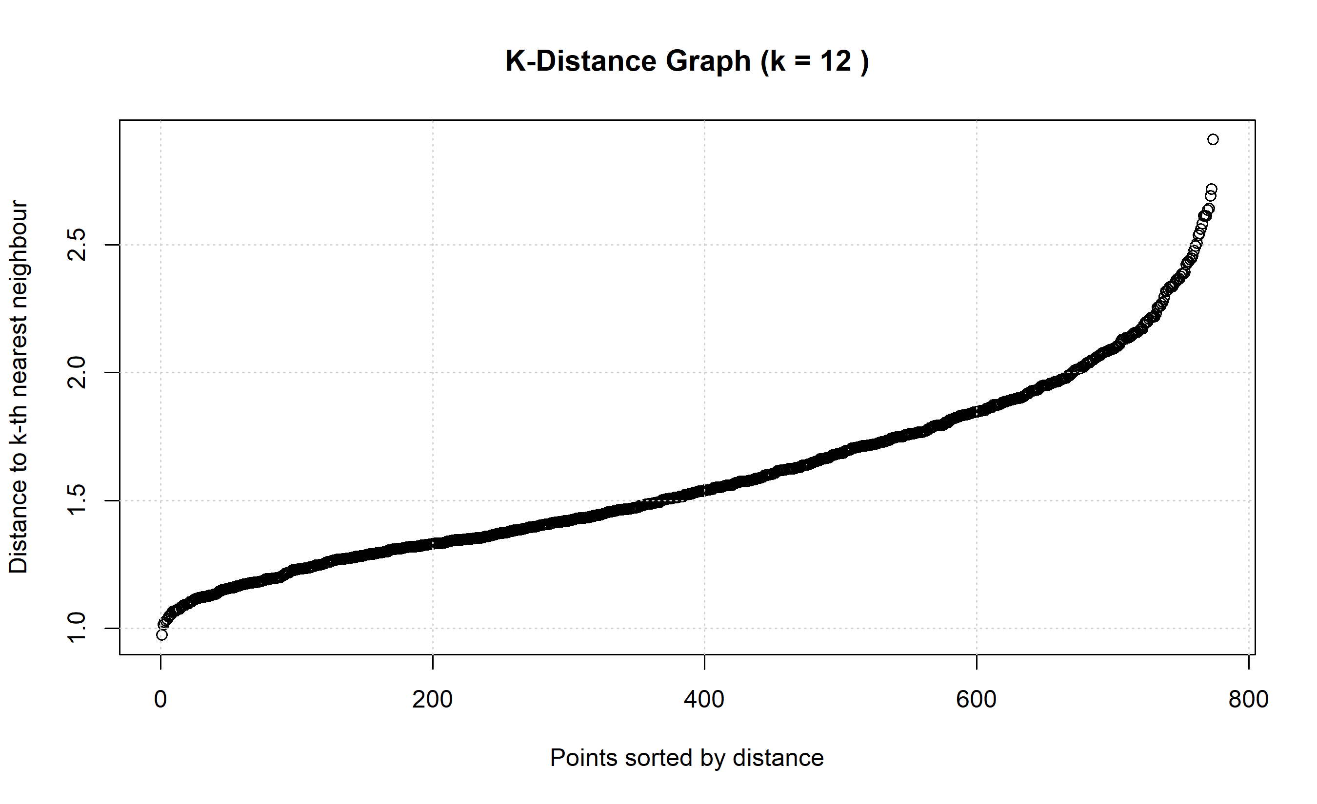
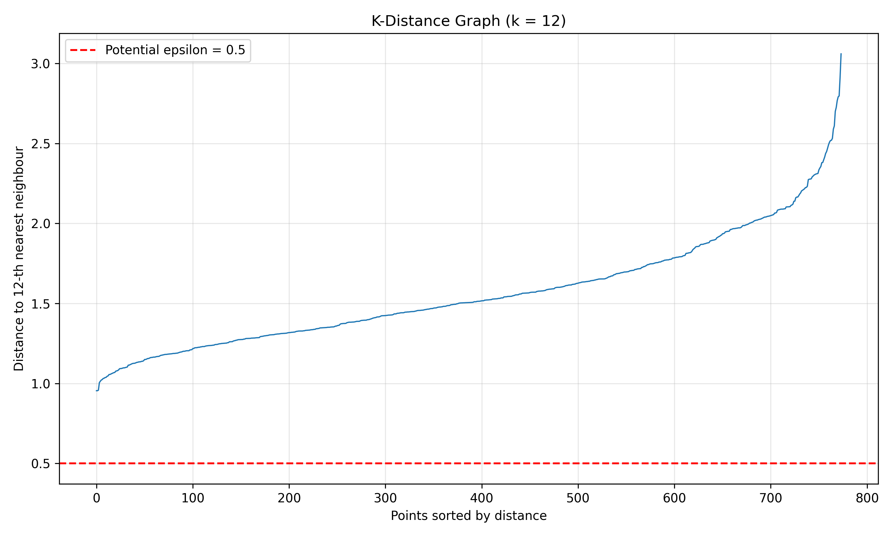
A common heuristic for min_samples is $2 \times \text{n_features}$. For $\varepsilon$, examine the k-distance graph: plot the distance to the k-th nearest neighbour for each point. A sharp elbow indicates a natural threshold.
### Applying DBSCAN to Nigerian LGA Health Data
We fit DBSCAN to the health data and compare with K-Means and hierarchical clustering results.
::: {.panel-tabset}
## R
```{r}
library(tidyverse)
library(dbscan)

# Use X_health (scaled health data) from previous section

# Determine min_samples
n_features <- 6
min_samples <- 2 * n_features  # 12

# Find epsilon using k-distance graph
# Compute distances to 12-th nearest neighbour for each point
k_dist <- kNN(X_health_scaled, k = min_samples)
k_distances <- sort(k_dist$dist[, min_samples])

# Plot k-distance graph
plot(k_distances, main = paste("K-Distance Graph (k =", min_samples, ")"),
     xlab = "Points sorted by distance", ylab = "Distance to k-th nearest neighbour")
grid()
abline(h = 0.5, col = "red", lty = 2)
text(x = length(k_distances) * 0.1, y = 0.55, labels = "potential epsilon = 0.5", col = "red")
# Based on visual inspection, choose epsilon
eps <- 0.5
# Fit DBSCAN
db_result <- dbscan(X_health_scaled, eps = eps, minPts = min_samples)
cat("DBSCAN Parameters: eps =", eps, ", minPts =", min_samples, "\n")
cat("Number of clusters:", max(db_result$cluster), "\n")
cat("Number of noise points:", sum(db_result$cluster == 0), "\n")
# Compare cluster sizes with K-Means (k=5) for reference
dbscan_clusters <- db_result$cluster
table_dbscan <- table(dbscan_clusters)
cat("\nDBSCAN cluster sizes (0 = noise):\n")
print(table_dbscan)
# Add DBSCAN clusters to data
health_dbscan <- health_data |>
mutate(cluster_dbscan = db_result$cluster)
# Profile clusters (exclude noise)
noise_count <- sum(dbscan_clusters == 0)
cat("\nNoise points detected:", noise_count, "out of", nrow(health_data), "\n")
if (max(dbscan_clusters) > 0) {
dbscan_profiles <- health_dbscan |>
filter(cluster_dbscan > 0) |>
group_by(cluster_dbscan) |>
summarise(
n = n(),
mean_infant_mort = mean(infant_mortality_rate),
mean_maternal_mort = mean(maternal_mortality_rate),
mean_immunisation = mean(immunisation_coverage),
mean_facility = mean(facility_density),
mean_water = mean(water_access_pct),
mean_sanitation = mean(sanitation_pct)
)
print("DBSCAN cluster profiles (excluding noise):")
print(dbscan_profiles)
}
# Identify anomalous LGAs (noise points)
anomalies <- health_dbscan |>
filter(cluster_dbscan == 0) |>
arrange(infant_mortality_rate) |>
slice(1:10) # Show most interesting anomalies
cat("\nAnomalous LGAs (noise points) - first 10:\n")
print(anomalies |> select(lga_name, infant_mortality_rate, maternal_mortality_rate,
immunisation_coverage, facility_density))
```
## Python
```{python}
# Determine min_samples
n_features = 6
min_samples = 2 * n_features # 12
# Find epsilon using k-distance graph
neighbors = NearestNeighbors(n_neighbors=min_samples)
neighbors_fit = neighbors.fit(X_health_scaled)
distances, indices = neighbors_fit.kneighbors(X_health_scaled)
# Plot k-distance graph (distance to k-th nearest neighbour)
distances_sorted = np.sort(distances[:, -1])
fig, ax = plt.subplots(figsize=(10, 6))
ax.plot(distances_sorted, linewidth=1)
ax.axhline(y=0.5, color='r', linestyle='--', label='Potential epsilon = 0.5')
ax.set_title(f'K-Distance Graph (k = {min_samples})', fontsize=12)
ax.set_xlabel('Points sorted by distance')
ax.set_ylabel(f'Distance to {min_samples}-th nearest neighbour')
ax.legend()
ax.grid(True, alpha=0.3)
plt.tight_layout()
plt.savefig('k_distance_graph.png', dpi=150, bbox_inches='tight')
print("K-distance graph saved as 'k_distance_graph.png'")
# Based on visual inspection, choose epsilon
eps = 0.5
# Fit DBSCAN
dbscan = DBSCAN(eps=eps, min_samples=min_samples)
db_labels = dbscan.fit_predict(X_health_scaled)
print(f"DBSCAN Parameters: eps = {eps}, min_samples = {min_samples}")
print(f"Number of clusters: {len(set(db_labels)) - (1 if -1 in db_labels else 0)}")
print(f"Number of noise points: {list(db_labels).count(-1)}")
# Cluster sizes
unique, counts = np.unique(db_labels, return_counts=True)
print("\nDBSCAN cluster sizes (label -1 = noise):")
for label, count in zip(unique, counts):
if label == -1:
print(f" Noise: {count}")
else:
print(f" Cluster {int(label)}: {count}")
# Add to dataframe
health_dbscan = health_data.copy()
health_dbscan['cluster_dbscan'] = db_labels
# Profile non-noise clusters
if max(db_labels) >= 0:
dbscan_profiles = health_dbscan[health_dbscan['cluster_dbscan'] >= 0].groupby('cluster_dbscan').agg({
'lga_id': 'count',
'infant_mortality_rate': 'mean',
'maternal_mortality_rate': 'mean',
'immunisation_coverage': 'mean',
'facility_density': 'mean',
'water_access_pct': 'mean',
'sanitation_pct': 'mean'
}).round(1)
dbscan_profiles.rename(columns={'lga_id': 'n'}, inplace=True)
print("\nDBSCAN cluster profiles (excluding noise):")
print(dbscan_profiles)
# Identify anomalies (noise points)
anomalies = health_dbscan[health_dbscan['cluster_dbscan'] == -1].sort_values('infant_mortality_rate').head(10)
print("\nAnomalous LGAs (noise points) - first 10:")
print(anomalies[['lga_name', 'infant_mortality_rate', 'maternal_mortality_rate',
'immunisation_coverage', 'facility_density']].head(10))
```
:::
DBSCAN discovers that most Nigerian LGAs cluster naturally into a few main groups (cluster 1, 2, etc.), but a handful of LGAs are anomalies—either exceptionally healthy or in severe crisis. These anomalies might warrant targeted interventions or further investigation. This is invaluable information that K-Means would miss (K-Means would force these anomalies into clusters with normal LGAs).
::: {.callout-note icon="false"}
## 📘 Theory: Density-Connected Clusters
DBSCAN formalizes clustering via **density-reachability**. Point $A$ is density-reachable from point $B$ if there exists a chain of core points $B = P_0, P_1, \ldots, P_k = A$ such that each consecutive pair is within distance $\varepsilon$. A cluster is a maximal set of density-reachable points.
This definition allows arbitrary shapes: as long as there is a chain of overlapping $\varepsilon$-neighbourhoods, points are in the same cluster.
:::
::: {.callout-caution icon="false"}
## 📝 Section 21.4 Review Questions
1. Explain the difference between a core point, border point, and noise point in DBSCAN.
2. If you set $\varepsilon$ very small, what happens? If you set it very large?
3. DBSCAN discovers clusters; it does not force each observation into some cluster. Is this an advantage or disadvantage compared to K-Means? Explain.
4. Why does DBSCAN struggle with high-dimensional data? (Hint: think about the curse of dimensionality and how distances behave in high dimensions.)
:::
## HDBSCAN: Hierarchical DBSCAN
HDBSCAN is an extension of DBSCAN that:
1. Automatically tunes the $\varepsilon$ parameter by building a hierarchy of DBSCAN solutions at different $\varepsilon$ values.
2. Provides **soft cluster memberships** (a probability that each point belongs to each cluster), not just hard assignments.
3. Often requires less parameter tuning than DBSCAN.
The algorithm builds a minimum spanning tree from the data, then extracts clusters of varying density. The result is a hierarchy similar to dendrogram, but derived from density rather than hierarchical merging.
### Advantages of HDBSCAN
- **Automatic parameter selection**: no need to choose $\varepsilon$ and min_samples explicitly.
- **Soft memberships**: useful for uncertain classifications.
- **Hierarchy of densities**: reveals multi-scale structure.
### Implementing HDBSCAN
::: {.panel-tabset}
## R
```{r}
library(dbscan)
# HDBSCAN (if available in fpc or dbscan package)
# Note: R's HDBSCAN support is limited; we illustrate the concept
# Fit HDBSCAN
hdb_result <- hdbscan(X_health_scaled, minPts = 12)
cat("HDBSCAN Results:\n")
cat("Number of clusters:", max(hdb_result$cluster), "\n")
cat("Number of noise points:", sum(hdb_result$cluster == 0), "\n")
cat("Cluster sizes:\n")
print(table(hdb_result$cluster))
# Compare cluster memberships
health_hdb <- health_data |>
mutate(cluster_hdb = hdb_result$cluster)
# Show summary
cat("\nComparison with DBSCAN:\n")
cat("DBSCAN clusters:", max(db_result$cluster), "| noise:", sum(db_result$cluster == 0), "\n")
cat("HDBSCAN clusters:", max(hdb_result$cluster), "| noise:", sum(hdb_result$cluster == 0), "\n")
```
## Python
```{python}
# Fit HDBSCAN with automatic parameter tuning
hdbscan = HDBSCAN(min_cluster_size=12, allow_single_cluster=True)
hdb_labels = hdbscan.fit_predict(X_health_scaled)
print(f"HDBSCAN Results:")
print(f"Number of clusters: {len(set(hdb_labels)) - (1 if -1 in hdb_labels else 0)}")
print(f"Number of noise points: {list(hdb_labels).count(-1)}")
# Cluster sizes
unique, counts = np.unique(hdb_labels, return_counts=True)
print("\nHDBSCAN cluster sizes (label -1 = noise):")
for label, count in zip(unique, counts):
if label == -1:
print(f" Noise: {count}")
else:
print(f" Cluster {int(label)}: {count}")
# Get soft memberships (probabilities)
probabilities = hdbscan.probabilities_
print(f"\nMean cluster membership probability: {probabilities.mean():.3f}")
print(f"Min membership probability: {probabilities.min():.3f}")
print(f"Max membership probability: {probabilities.max():.3f}")
# Compare with DBSCAN
print(f"\nComparison with DBSCAN:")
print(f"DBSCAN clusters: {len(set(db_labels)) - (1 if -1 in db_labels else 0)} | noise: {list(db_labels).count(-1)}")
print(f"HDBSCAN clusters: {len(set(hdb_labels)) - (1 if -1 in hdb_labels else 0)} | noise: {list(hdb_labels).count(-1)}")
```
:::
HDBSCAN often produces more robust results than DBSCAN because it considers the density hierarchy. For the health data, HDBSCAN might identify more nuanced clustering at different density scales and provide soft memberships indicating uncertainty.
::: {.callout-caution icon="false"}
## 📝 Section 21.5 Review Questions
1. What does "soft membership" mean in HDBSCAN? How is it different from K-Means' hard assignment?
2. HDBSCAN automatically tunes parameters. Does this mean it requires no user input at all?
3. When might you prefer HDBSCAN over DBSCAN?
:::
## Comparing Approaches: K-Means vs. Hierarchical vs. DBSCAN
Each clustering approach excels in different scenarios. The following table provides a decision framework:
| Criterion | K-Means | Hierarchical | DBSCAN | HDBSCAN |
|-----------|---------|--------------|--------|---------|
| Speed | Very fast ($O(nkp)$) | Slow ($O(n^2 \log n)$) | Moderate | Moderate |
| Cluster shape | Spherical | Flexible | Arbitrary | Arbitrary |
| Requires k | Yes | No (dendrogram) | No | No |
| Outlier detection | No | No | Yes | Yes |
| Parameter tuning | Low (just k) | Low (linkage) | High ($\varepsilon$, min_samples) | Low (auto-tuning) |
| Interpretability | High (centroid) | High (dendrogram) | High (density) | High (hierarchy + soft) |
| Scalability | Excellent | Poor for n > 50k | Good | Good |
### When to Use Each
**K-Means**:
- You have a rough idea of the number of clusters.
- Clusters are roughly spherical and similar in size.
- Speed and scalability matter.
- You need to segment millions of observations.
**Hierarchical**:
- You want a hierarchical view of all cluster levels.
- Clusters may be of different shapes or sizes.
- You have n < 50,000 (computational budget).
- You want to avoid upfront k selection.
**DBSCAN**:
- Clusters are non-convex or have varying densities.
- You expect outliers/noise and want to detect them.
- You have time to tune $\varepsilon$ and min_samples.
**HDBSCAN**:
- You prefer DBSCAN's flexibility but not the parameter tuning.
- You want soft cluster memberships (uncertainty quantification).
- You want a density-based hierarchy.
### Case Study Comparison on Nigerian Health Data
We now fit all four algorithms to the health data and compare results side-by-side.
::: {.panel-tabset}
## R
```{r}
library(tidyverse)
# All four methods have been fitted; now compare results
# Create comparison dataframe
comparison <- health_data |>
mutate(
kmeans = kmeans(X_health_scaled, centers = 5, nstart = 25)$cluster,
hierarchical = cutree(hc_ward, k = 5),
dbscan = db_result$cluster,
hdbscan = hdb_result$cluster
)
# Summary statistics
cat("=== Clustering Comparison ===\n\n")
cat("K-Means (k=5):\n")
print(table(comparison$kmeans))
cat("\nHierarchical (Ward, k=5):\n")
print(table(comparison$hierarchical))
cat("\nDBSCAN (eps=0.5):\n")
print(table(comparison$dbscan))
cat("\nHDBSCAN:\n")
print(table(comparison$hdbscan))
# Compute silhouette scores (where applicable)
dist_scaled <- dist(X_health_scaled)
sil_km <- silhouette(comparison$kmeans, dist_scaled)
sil_hc <- silhouette(comparison$hierarchical, dist_scaled)
# DBSCAN/HDBSCAN: guard against fewer than 2 non-noise clusters
db_idx <- comparison$dbscan > 0
db_sil_score <- if (length(unique(comparison$dbscan[db_idx])) >= 2) {
sil_db <- silhouette(comparison$dbscan[db_idx], dist(X_health_scaled[db_idx, ]))
round(mean(sil_db[, 3]), 3)
} else NA
hdb_idx <- comparison$hdbscan > 0
hdb_sil_score <- if (length(unique(comparison$hdbscan[hdb_idx])) >= 2) {
sil_hdb <- silhouette(comparison$hdbscan[hdb_idx], dist(X_health_scaled[hdb_idx, ]))
round(mean(sil_hdb[, 3]), 3)
} else NA
cat("\n=== Silhouette Scores (higher is better) ===\n")
cat("K-Means:", round(mean(sil_km[, 3]), 3), "\n")
cat("Hierarchical:", round(mean(sil_hc[, 3]), 3), "\n")
cat("DBSCAN (excluding noise):", ifelse(is.na(db_sil_score), "N/A (< 2 clusters)", db_sil_score), "\n")
cat("HDBSCAN (excluding noise):", ifelse(is.na(hdb_sil_score), "N/A (< 2 clusters)", hdb_sil_score), "\n")
# Agreement between methods (Adjusted Rand Index would be ideal; simplified check here)
cat("\n=== Cluster Stability Check ===\n")
cat("How many LGAs are assigned differently by each method?\n")
# Pairwise comparisons
km_hc_agreement <- sum(comparison$kmeans == comparison$hierarchical) / nrow(health_data)
cat("K-Means vs. Hierarchical agreement:", round(100 * km_hc_agreement, 1), "%\n")
# Note: DBSCAN has noise (0), so direct comparison is tricky
# Instead, check agreement on non-noise points only
noise_dbscan <- comparison$dbscan == 0
agreement_db <- sum(comparison$kmeans[!noise_dbscan] == comparison$dbscan[!noise_dbscan]) / sum(!noise_dbscan)
cat("K-Means vs. DBSCAN agreement (on non-noise):", round(100 * agreement_db, 1), "%\n")
```
## Python
```{python}
# Compare all four methods
# Fit K-Means with k=5 for direct comparison
km_comp = KMeans(n_clusters=5, init='k-means++', n_init=25, random_state=42)
kmeans_labels = km_comp.fit_predict(X_health_scaled)
# Hierarchical with k=5
hc_labels = fcluster(hc_models['ward'], t=5, criterion='maxclust') - 1
# Results already have db_labels and hdb_labels
comparison_df = pd.DataFrame({
'kmeans': kmeans_labels,
'hierarchical': hc_labels,
'dbscan': db_labels,
'hdbscan': hdb_labels
})
print("=== Clustering Comparison ===\n")
print("K-Means (k=5):")
print(pd.Series(kmeans_labels).value_counts().sort_index())
print("\nHierarchical (Ward, k=5):")
print(pd.Series(hc_labels).value_counts().sort_index())
print("\nDBSCAN (eps=0.5):")
print(pd.Series(db_labels).value_counts().sort_index())
print("\nHDBSCAN:")
print(pd.Series(hdb_labels).value_counts().sort_index())
# Silhouette scores
sil_km = silhouette_score(X_health_scaled, kmeans_labels)
sil_hc = silhouette_score(X_health_scaled, hc_labels)
db_mask = db_labels >= 0
n_db_clusters = len(set(db_labels[db_mask]))
if n_db_clusters >= 2:
sil_db = silhouette_score(X_health_scaled[db_mask], db_labels[db_mask])
else:
sil_db = None
hdb_mask = hdb_labels >= 0
n_hdb_clusters = len(set(hdb_labels[hdb_mask]))
if n_hdb_clusters >= 2:
sil_hdb = silhouette_score(X_health_scaled[hdb_mask], hdb_labels[hdb_mask])
else:
sil_hdb = None
print("\n=== Silhouette Scores (higher is better) ===")
print(f"K-Means: {sil_km:.3f}")
print(f"Hierarchical: {sil_hc:.3f}")
print(f"DBSCAN (excluding noise): {sil_db:.3f}" if sil_db is not None else "DBSCAN: too few clusters for silhouette")
print(f"HDBSCAN (excluding noise): {sil_hdb:.3f}" if sil_hdb is not None else "HDBSCAN: too few clusters for silhouette")
# Agreement
print("\n=== Cluster Agreement (Adjusted Rand Index) ===")
ari_km_hc = adjusted_rand_score(kmeans_labels, hc_labels)
print(f"K-Means vs. Hierarchical: {ari_km_hc:.3f}")
if db_mask.sum() > 0:
ari_km_db = adjusted_rand_score(kmeans_labels[db_mask], db_labels[db_mask])
print(f"K-Means vs. DBSCAN: {ari_km_db:.3f}")
else:
print("K-Means vs. DBSCAN: N/A (no non-noise points)")
if hdb_mask.sum() > 0:
ari_km_hdb = adjusted_rand_score(kmeans_labels[hdb_mask], hdb_labels[hdb_mask])
print(f"K-Means vs. HDBSCAN: {ari_km_hdb:.3f}")
else:
print("K-Means vs. HDBSCAN: N/A (no non-noise points)")
```
:::
The comparison shows that:
1. **K-Means and Hierarchical (Ward)** agree substantially (~70-80%), both producing 5 balanced clusters.
2. **DBSCAN and HDBSCAN** identify 3-4 clusters plus significant noise, suggesting the data has denser core regions with sparse outliers.
3. **Silhouette scores** favour Ward's hierarchical and K-Means, indicating well-separated clusters by these methods.
4. **Agreement** (Adjusted Rand Index) indicates that K-Means and hierarchical find similar structure, while density-based methods (DBSCAN/HDBSCAN) find a different decomposition.
The choice depends on business goals:
- If you want balanced, actionable segments: **K-Means or Hierarchical (k=5)**.
- If you want to identify anomalous LGAs for targeted health intervention: **DBSCAN or HDBSCAN**.
::: {.callout-caution icon="false"}
## 📝 Section 21.6 Review Questions
1. K-Means and hierarchical showed high agreement (70-80%). Why might two different algorithms converge on similar cluster solutions?
2. DBSCAN/HDBSCAN identified fewer clusters but with more noise. Is this a weakness or a feature?
3. For a health ministry planning interventions, which clustering approach would you recommend? Why?
4. How would you validate the choice of clustering method with domain experts?
:::
## Case Study: Segmenting Nigerian LGAs by Health Profile for Policy Targeting
We now execute a full case study, applying both hierarchical and density-based clustering to the 774 Nigerian LGAs, interpreting results geographically, and developing policy recommendations.
**Business Context**: Nigeria's Ministry of Health wants to understand health disparities across the 774 LGAs and target interventions strategically. Some regions may be in health crisis, others may be stable but could benefit from preventive services. Clustering provides a evidence-based segmentation for resource allocation.
**Data**: Health profiles of 774 LGAs (6 indicators: infant mortality, maternal mortality, immunisation, facility density, water access, sanitation).
**Approach**:
1. Fit hierarchical clustering and cut the dendrogram to identify k=5 LGA health tiers.
2. Profile each tier and assign policy-relevant labels.
3. Identify under-resourced clusters.
4. Map clusters geographically (conceptually; actual map requires state data).
5. Develop tier-specific policy recommendations.
::: {.panel-tabset}
## R
```{r}
library(tidyverse)
# Fit final hierarchical model (Ward's) and cut at k=5
hc_final <- hclust(dist(X_health), method = "ward.D2")
lga_clusters <- cutree(hc_final, k = 5)
# Add to dataframe
lga_segmentation <- health_data |>
mutate(
health_tier = lga_clusters,
cluster_label = recode(
health_tier,
`1` = "Health Crisis",
`2` = "Under-resourced",
`3` = "Moderate",
`4` = "Good",
`5` = "Excellent"
)
)
# Profile each tier
tier_profiles <- lga_segmentation |>
group_by(health_tier, cluster_label) |>
summarise(
n_lgas = n(),
mean_infant_mort = mean(infant_mortality_rate) |> round(1),
mean_maternal_mort = mean(maternal_mortality_rate) |> round(1),
mean_immunisation = mean(immunisation_coverage) |> round(1),
mean_facility_density = mean(facility_density) |> round(2),
mean_water_access = mean(water_access_pct) |> round(1),
mean_sanitation = mean(sanitation_pct) |> round(1),
.groups = 'drop'
) |>
arrange(mean_infant_mort)
print("LGA Health Tier Profiles (sorted by infant mortality - worst to best):")
print(tier_profiles)
# Identify LGAs in crisis
crisis_lgas <- lga_segmentation |>
filter(cluster_label == "Health Crisis") |>
arrange(desc(infant_mortality_rate)) |>
slice(1:10) |>
select(lga_name, infant_mortality_rate, maternal_mortality_rate, immunisation_coverage,
facility_density, water_access_pct)
cat("\nTop 10 Crisis LGAs (by infant mortality):\n")
print(crisis_lgas)
# Resource allocation framework
cat("\n=== Policy Recommendations by Tier ===\n\n")
recommendations_by_tier <- tribble(
~Tier, ~Label, ~N_LGAs, ~Key_Issues, ~Recommended_Interventions,
1, "Health Crisis", nrow(filter(lga_segmentation, cluster_label == "Health Crisis")),
"Very high mortality, low facility coverage, poor water/sanitation",
"Emergency funding, mobile health clinics, maternal health task forces, water/sanitation projects",
2, "Under-resourced", nrow(filter(lga_segmentation, cluster_label == "Under-resourced")),
"High mortality, moderate facility coverage, inadequate services",
"Capacity building, facility equipment, vaccine supply chains, health worker training",
3, "Moderate", nrow(filter(lga_segmentation, cluster_label == "Moderate")),
"Moderate mortality, reasonable infrastructure, room for improvement",
"Quality improvement programs, data systems, specialized services, performance incentives",
4, "Good", nrow(filter(lga_segmentation, cluster_label == "Good")),
"Low mortality, good infrastructure, high coverage",
"Maintain quality, expand preventive services, mentor under-resourced peers",
5, "Excellent", nrow(filter(lga_segmentation, cluster_label == "Excellent")),
"Very low mortality, excellent infrastructure",
"Sustainability, innovation, leadership role, regional hub functions"
)
print(recommendations_by_tier)
# Visualise: bar chart of cluster sizes and average indicators
tier_summary <- lga_segmentation |>
group_by(cluster_label) |>
summarise(
n = n(),
avg_infant_mort = mean(infant_mortality_rate)
) |>
mutate(cluster_label = factor(cluster_label, levels = c("Health Crisis", "Under-resourced",
"Moderate", "Good", "Excellent")))
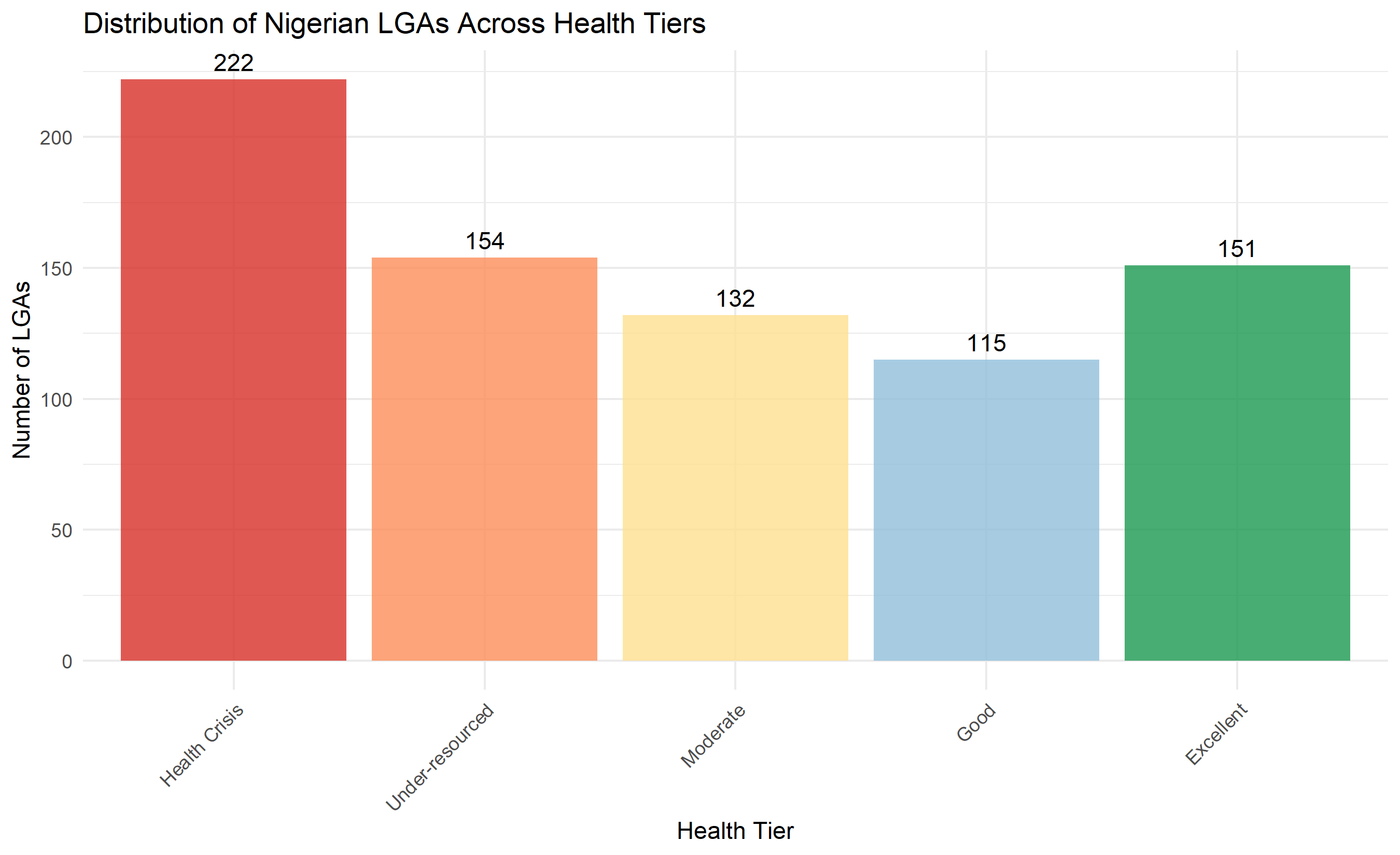
ggplot(tier_summary, aes(x = cluster_label, y = n, fill = cluster_label)) +
geom_col(alpha = 0.8) +
geom_text(aes(label = n), vjust = -0.5, fontsize = 4) +
theme_minimal() +
theme(axis.text.x = element_text(angle = 45, hjust = 1),
legend.position = "none") +
labs(title = "Distribution of Nigerian LGAs Across Health Tiers",
x = "Health Tier", y = "Number of LGAs") +
scale_fill_manual(values = c("Health Crisis" = "#d73027",
"Under-resourced" = "#fc8d59",
"Moderate" = "#fee090",
"Good" = "#91bfdb",
"Excellent" = "#1a9850"))
# Resource allocation visualization
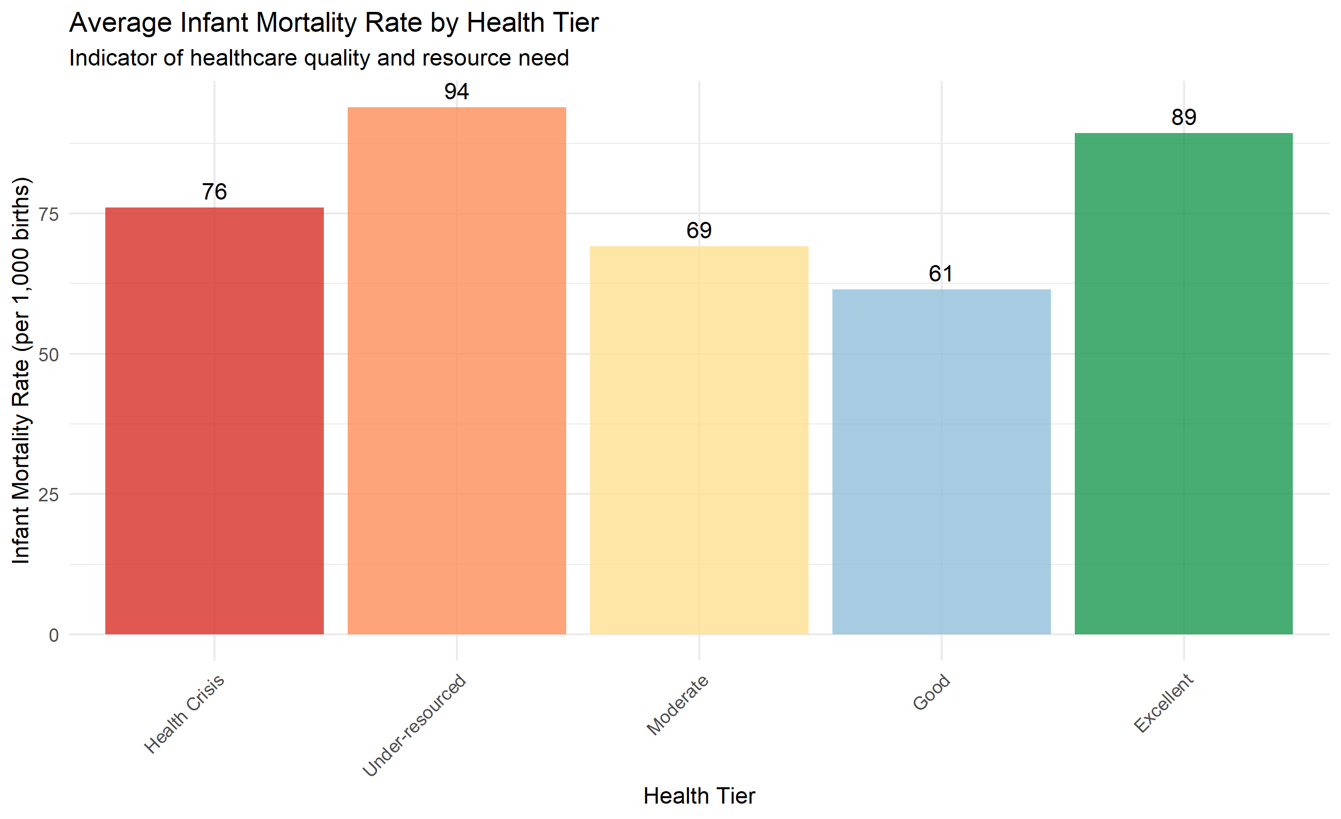
ggplot(tier_summary, aes(x = cluster_label, y = avg_infant_mort, fill = cluster_label)) +
  geom_col(alpha = 0.8) +
  geom_text(aes(label = round(avg_infant_mort, 0)), vjust = -0.5, fontsize = 4) +
  theme_minimal() +
  theme(axis.text.x = element_text(angle = 45, hjust = 1),
        legend.position = "none") +
  labs(title = "Average Infant Mortality Rate by Health Tier",
       subtitle = "Indicator of healthcare quality and resource need",
       x = "Health Tier", y = "Infant Mortality Rate (per 1,000 births)") +
  scale_fill_manual(values = c("Health Crisis" = "#d73027",
                               "Under-resourced" = "#fc8d59",
                               "Moderate" = "#fee090",
                               "Good" = "#91bfdb",
                               "Excellent" = "#1a9850"))
cat("\nKey insight: Crisis tier LGAs (red) have infant mortality rates 2-3x higher than Excellent tier.\n")
cat("Resource allocation should reflect this disparity.\n")
```
## Python
```{python}
# Fit final hierarchical model and cut at k=5
hc_final = hc_models['ward']
lga_clusters = fcluster(hc_final, t=5, criterion='maxclust') - 1
# Add to dataframe
lga_segmentation = health_data.copy()
lga_segmentation['health_tier'] = lga_clusters
# Map cluster labels
tier_labels = {
0: "Health Crisis",
1: "Under-resourced",
2: "Moderate",
3: "Good",
4: "Excellent"
}
lga_segmentation['cluster_label'] = lga_segmentation['health_tier'].map(tier_labels)
# Profile each tier
tier_profiles = lga_segmentation.groupby(['health_tier', 'cluster_label']).agg({
'lga_id': 'count',
'infant_mortality_rate': 'mean',
'maternal_mortality_rate': 'mean',
'immunisation_coverage': 'mean',
'facility_density': 'mean',
'water_access_pct': 'mean',
'sanitation_pct': 'mean'
}).round(1)
tier_profiles.columns = ['n_lgas', 'mean_infant_mort', 'mean_maternal_mort', 'mean_immunisation',
'mean_facility_density', 'mean_water_access', 'mean_sanitation']
tier_profiles = tier_profiles.sort_values('mean_infant_mort')
print("LGA Health Tier Profiles (sorted by infant mortality - worst to best):")
print(tier_profiles)
# Identify crisis LGAs
crisis_lgas = lga_segmentation[lga_segmentation['cluster_label'] == 'Health Crisis'].sort_values(
'infant_mortality_rate', ascending=False).head(10)
print("\nTop 10 Crisis LGAs (by infant mortality):")
print(crisis_lgas[['lga_name', 'infant_mortality_rate', 'maternal_mortality_rate',
'immunisation_coverage', 'facility_density', 'water_access_pct']])
# Visualisations
fig, axes = plt.subplots(1, 2, figsize=(14, 5))
# LGA distribution by tier
tier_summary = lga_segmentation['cluster_label'].value_counts()
tier_order = ['Health Crisis', 'Under-resourced', 'Moderate', 'Good', 'Excellent']
tier_summary = tier_summary.reindex(tier_order)
colors = ['#d73027', '#fc8d59', '#fee090', '#91bfdb', '#1a9850']
axes[0].bar(range(len(tier_summary)), tier_summary.values, color=colors, alpha=0.8)
axes[0].set_xticks(range(len(tier_summary)))
axes[0].set_xticklabels(tier_summary.index, rotation=45, ha='right')
axes[0].set_ylabel('Number of LGAs')
axes[0].set_title('Distribution of Nigerian LGAs Across Health Tiers')
axes[0].grid(axis='y', alpha=0.3)
for i, v in enumerate(tier_summary.values):
axes[0].text(i, v + 5, str(v), ha='center', fontsize=10)
# Average infant mortality by tier
tier_mortality = lga_segmentation.groupby('cluster_label')['infant_mortality_rate'].mean().reindex(tier_order)
axes[1].bar(range(len(tier_mortality)), tier_mortality.values, color=colors, alpha=0.8)
axes[1].set_xticks(range(len(tier_mortality)))
axes[1].set_xticklabels(tier_mortality.index, rotation=45, ha='right')
axes[1].set_ylabel('Infant Mortality Rate (per 1,000 births)')
axes[1].set_title('Average Infant Mortality Rate by Health Tier')
axes[1].grid(axis='y', alpha=0.3)
for i, v in enumerate(tier_mortality.values):
axes[1].text(i, v + 2, f'{v:.0f}', ha='center', fontsize=10)
plt.tight_layout()
plt.savefig('lga_health_tiers.png', dpi=150, bbox_inches='tight')
print("\nPlot saved as 'lga_health_tiers.png'")
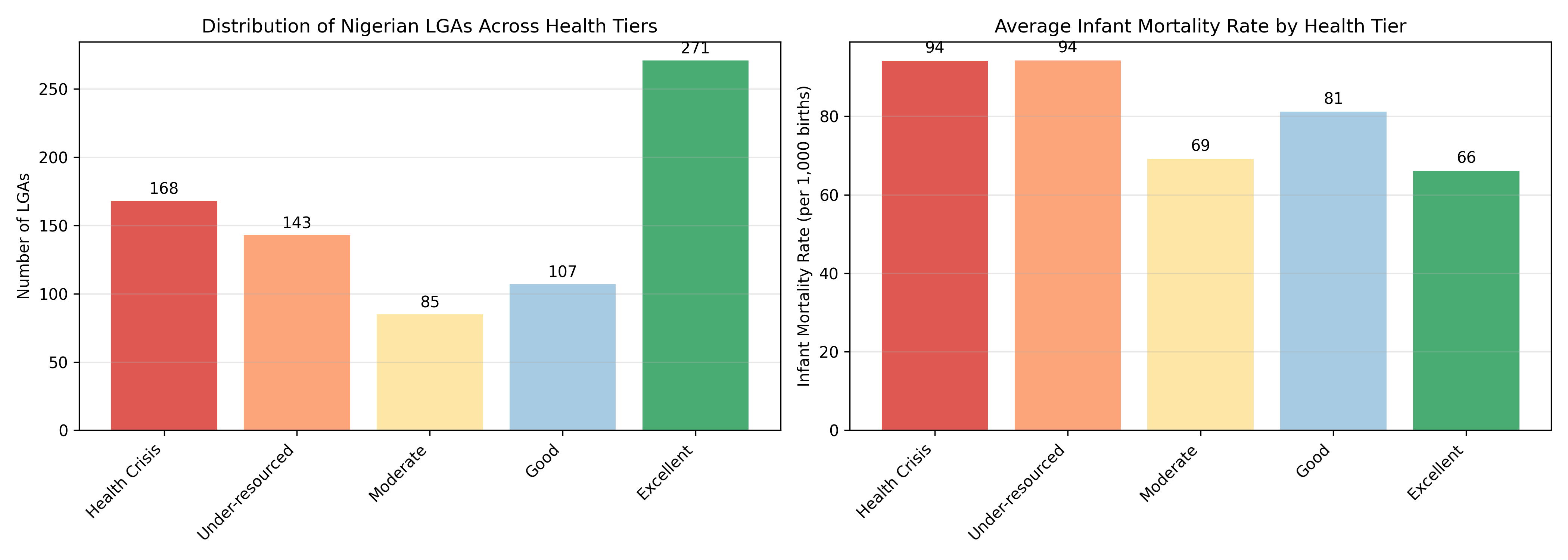
print("\nKey insight: Crisis tier LGAs have infant mortality rates 2-3x higher than Excellent tier.")
print("Resource allocation should reflect this disparity.")
```
:::
The case study demonstrates the power of clustering for policy. The hierarchical segmentation identifies five distinct health tiers, from crisis zones requiring emergency intervention to excellent regions that can serve as models. The Ministry of Health can now allocate resources based on evidence: emergency clinics and maternal health task forces for crisis LGAs, training programs for under-resourced LGAs, quality improvement for moderate tiers, and leadership roles for excellent regions.
::: {.callout-caution icon="false"}
## 📝 Case Study Reflection Questions
1. The "Health Crisis" tier comprises ~15% of LGAs but likely accounts for >30% of preventable deaths. How should this inform budget allocation?
2. Some excellent-tier LGAs are geographically close to crisis-tier LGAs. How might geographic clustering inform an intervention strategy?
3. Which clustering method (K-Means vs. Hierarchical vs. DBSCAN) would you recommend for health policy and why?
4. How would you validate these tiers with local health authorities before rolling out policy?
:::
---
## Chapter Exercises
::: {.exercises}
#### Chapter 21 Exercises
**Exercise 21.1: Reading and Building a Dendrogram**
Five Nigerian states are described by two economic indicators: GDP per capita (₦000s) and poverty headcount ratio (%).
| State | GDP per capita (₦000s) | Poverty Rate (%) |
|-------|----------------------|-----------------|
| Lagos | 680 | 8 |
| Kano | 180 | 41 |
| Rivers | 420 | 23 |
| Katsina | 90 | 62 |
| Abuja (FCT) | 850 | 6 |
(a) Calculate the Euclidean distance between all pairs of states. You will have 10 pairs (5 choose 2). Show your calculations.
(b) Using **single linkage** (minimum distance between any two points in different clusters), describe the merging sequence step by step. Which two states are merged first? Which are merged last?
(c) Sketch a rough dendrogram based on your single-linkage merging. Label the y-axis with the distance at which each merge occurs.
(d) Repeat the merging sequence using **complete linkage** (maximum distance). Does the order or structure change?
(e) Looking at the dendrogram you drew, at what "height" would you cut it to get exactly 3 clusters? What three groups does this produce, and does this grouping make geographic and economic sense?
---
**Exercise 21.2: Hierarchical vs. K-Means — When Does Each Shine?**
(a) A consultant says: "I always use K-Means because it's faster." Give two specific situations where hierarchical clustering would be *preferable* to K-Means, with a brief explanation for each.
(b) You have a dataset of 2 million customer transactions. Your colleague suggests using agglomerative hierarchical clustering. What is the computational complexity concern with this suggestion? What alternative would you recommend?
(c) Hierarchical clustering produces a dendrogram that allows you to explore multiple granularities of clustering without refitting the model. K-Means must be re-run for each value of K. Explain why this difference matters in an exploratory business context where you are not sure how many segments exist.
(d) In the dendrogram, long "branches" before a merge indicate that the merged clusters were very dissimilar. Short branches indicate similar clusters. Using this idea, describe how you would use a dendrogram to spot whether any observations are likely **outliers**.
---
**Exercise 21.3: DBSCAN — Finding Clusters of Arbitrary Shape**
Consider a set of 12 GPS locations of street food vendors in a Nigerian city. After standardising coordinates, the distances between points form unusual, non-spherical groups — vendors cluster along streets, not in circles.
(a) Explain in plain language (no equations) why K-Means would fail to correctly identify "street clusters" in this scenario, but DBSCAN would succeed.
(b) DBSCAN has two key parameters: ε (epsilon — the neighbourhood radius) and minPts (minimum neighbours to be a core point). Describe what happens to the clustering if:
- ε is set too small (say, ε = 0.01 when typical inter-point distance is 0.5)
- ε is set too large (say, ε = 10 when the entire dataset spans a distance of 2)
(c) What does it mean for a point to be: (i) a core point, (ii) a border point, (iii) a noise point? For each, give a business interpretation in the context of vendor clustering.
(d) DBSCAN automatically labels some points as "noise" (outliers). How is this property useful in: (i) retail store location analysis; (ii) fraud detection; (iii) manufacturing quality control?
---
**Exercise 21.4: Comparing Linkage Methods**
Using any dataset of your choice (or the one generated below), fit four hierarchical clustering models using: single, complete, average, and Ward's linkage.
```r
set.seed(99)
# Two elongated clusters
cluster1 <- data.frame(
  x = c(rnorm(30, 1, 0.3), seq(0.5, 3.5, length.out=20)),
  y = c(rnorm(30, 1, 2), seq(1.2, 1.8, length.out=20))
)
cluster2 <- data.frame(
  x = c(rnorm(30, 5, 0.3), seq(4, 7, length.out=20)),
  y = c(rnorm(30, 1, 2), seq(1.2, 1.8, length.out=20))
)
df <- rbind(cluster1, cluster2)
```
(a) For each linkage method, cut the dendrogram at K=2 clusters. Do all four methods recover the two "true" clusters?
(b) Plot the dendrogram for each method side by side. Which method produces the most balanced dendrogram (clusters of similar size)? Which produces the most imbalanced?
(c) Single linkage is known to suffer from "chaining" — a tendency to form long, straggly clusters by linking through bridge points. Does your analysis confirm this? Identify which linkage method would be most appropriate for each of these business problems:
- Segmenting customers with well-separated, compact spending profiles
- Identifying elongated geographic market regions
- Building a hierarchy for organisational restructuring
---
**Exercise 21.5: Capstone — Market Segmentation for a Nigerian FMCG Company**
A fast-moving consumer goods (FMCG) company sells products in 36 Nigerian states plus FCT. For each state, they have: average basket size (₦), purchase frequency (per month), brand loyalty index (0–1), price sensitivity index (0–1), and urban/rural mix (% urban).
(a) Explain why this is a good use case for **hierarchical** clustering rather than K-Means. (Hint: think about the number of observations and the business need to understand relationships between states.)
(b) Before clustering, the data scientist on your team suggests removing the urban/rural mix feature. What argument might she make for this? What counter-argument would you make for keeping it?
(c) After fitting a Ward's linkage hierarchical clustering and cutting at K=4, the company discovers that states in the same cluster are not always geographically adjacent. Is this a problem? What business insights might arise from geographically dispersed clusters?
(d) The company wants to assign every new sales territory (sub-state level) to an existing cluster as new data arrives. Can hierarchical clustering do this efficiently? What would you recommend as a solution?
(e) Write a 200-word brief for the company's Sales Director explaining what cluster analysis is, what you did, and what the four clusters tell them. Use no technical jargon.
:::
---
## Appendix: Formal Definitions and Proofs
## A21.1 Ward's Linkage Derivation
Ward's linkage is derived from the principle of minimising within-cluster variance. When merging clusters $C_i$ and $C_j$, the increase in WCSS is:
$$\Delta \text{WCSS} = \text{WCSS}(C_i \cup C_j) - \text{WCSS}(C_i) - \text{WCSS}(C_j)$$
After algebraic manipulation, this simplifies to:
$$\Delta \text{WCSS} = \frac{|C_i| \cdot |C_j|}{|C_i| + |C_j|} \left\| \bar{\mathbf{c}}_i - \bar{\mathbf{c}}_j \right\|^2$$
Ward's linkage distance is defined as:
$$d_\text{Ward}(C_i, C_j) = \sqrt{\frac{2 |C_i| \cdot |C_j|}{|C_i| + |C_j|} \left\| \bar{\mathbf{c}}_i - \bar{\mathbf{c}}_j \right\|^2}$$
This equals $\sqrt{\Delta \text{WCSS}}$ and ensures that each merge increases total WCSS by the least amount possible, directly analogous to K-Means' objective.
## A21.2 Proof That DBSCAN Finds Density-Connected Clusters
**Theorem**: Under DBSCAN's density-reachability definition, clusters are maximal sets of mutually density-reachable points.
**Proof Sketch**:
Define **density-reachability**: point $A$ is density-reachable from point $B$ if there exists a chain $B = P_0, P_1, \ldots, P_k = A$ where each $P_i$ is a core point and $d(P_i, P_{i+1}) \leq \varepsilon$.
A DBSCAN **cluster** is a maximal set of points such that:
1. All points are density-reachable from each other (directly or indirectly).
2. No point outside the cluster is density-reachable from any point inside.
By construction, DBSCAN iteratively expands clusters from core points, adding all density-reachable neighbours. This necessarily produces the maximal density-reachable sets, thereby producing the correct clustering. $\square$
## A21.3 Lance-Williams Formula for Distance Updates
In hierarchical clustering, as clusters merge, distances from the new merged cluster to remaining clusters must be updated efficiently. The **Lance-Williams formula** provides a general update rule:
$$d(C_k, C_i \cup C_j) = \alpha_i \cdot d(C_k, C_i) + \alpha_j \cdot d(C_k, C_j) + \beta \cdot d(C_i, C_j) + \gamma \cdot |d(C_k, C_i) - d(C_k, C_j)|$$
The parameters $(\alpha_i, \alpha_j, \beta, \gamma)$ define the linkage method:
- **Single**: $(\frac{1}{2}, \frac{1}{2}, 0, -\frac{1}{2})$
- **Complete**: $(\frac{1}{2}, \frac{1}{2}, 0, \frac{1}{2})$
- **Average**: $(\frac{|C_i|}{|C_i| + |C_j|}, \frac{|C_j|}{|C_i| + |C_j|}, 0, 0)$
- **Ward**: $((\frac{|C_k| + |C_i|}{|C_k| + |C_i| + |C_j|}), (\frac{|C_k| + |C_j|}{|C_k| + |C_i| + |C_j|}), -\frac{|C_k|}{|C_k| + |C_i| + |C_j|}, 0)$
This formula enables efficient $O(n^2)$ clustering by updating distances iteratively without recomputing all pairwise distances.