---
title: "Sentiment Analysis"
---
```{python}
#| label: python-setup-28-sentiment-analysis
#| include: false
import numpy as np
import pandas as pd
import matplotlib.pyplot as plt
import seaborn as sns
from nltk.sentiment import SentimentIntensityAnalyzer
import nltk
from sklearn.feature_extraction.text import TfidfVectorizer
from sklearn.linear_model import LogisticRegression
from sklearn.preprocessing import LabelEncoder
from sklearn.metrics import confusion_matrix, precision_recall_fscore_support, classification_report
# transformers is optional (requires torch; install separately if needed)
try:
from transformers import pipeline as hf_pipeline
TRANSFORMERS_AVAILABLE = True
except ImportError:
TRANSFORMERS_AVAILABLE = False
hf_pipeline = None
```
::: {.callout-note icon="false"}
## 📋 Learning Objectives
- Understand the three levels of sentiment analysis: document polarity (positive/negative/neutral), aspect-level (opinions on features), and emotion classification
- Implement lexicon-based sentiment using VADER and AFINN, with handling of negation and intensifiers
- Build and evaluate a supervised sentiment classifier using logistic regression and TF-IDF
- Extract aspect-level sentiment from unstructured text using dependency parsing
- Apply pre-trained transformer models (RoBERTa, DistilBERT) for state-of-the-art sentiment prediction
- Address Nigerian Pidgin and multilingual sentiment challenges using code-switching-aware approaches
- Build an interactive sentiment monitoring dashboard for brand reputation tracking
:::
## What Sentiment Analysis Measures
Sentiment analysis quantifies subjective information in text. Three levels exist:
**Document Polarity**: Classifies an entire document as positive, negative, or neutral. A product review "This phone is excellent quality, great battery life" is positive; "The screen broke after one week" is negative. Useful for brand monitoring, customer satisfaction scoring, and feedback triage.
**Aspect-Level Sentiment**: Identifies opinions about specific features or aspects. "The design is sleek but the battery drains quickly" has mixed sentiment: positive on design, negative on battery. A restaurant review: "Food was delicious (aspect: quality, sentiment: positive), but service was slow (aspect: service, sentiment: negative)". Actionable for product development.
**Emotion Classification**: Beyond polarity, classifies discrete emotions. Ekman's six basic emotions: joy, sadness, anger, disgust, surprise, fear. A tweet "This is the best news ever! 🎉" expresses joy. "I can't believe they're shutting down the factory" expresses surprise and sadness. Useful for understanding emotional drivers of customer behaviour.
**Business Applications**:
- **Customer Service**: Triage incoming messages by severity (angry complaints vs. neutral inquiries).
- **Product Development**: Identify feature-level complaints for prioritisation.
- **Brand Monitoring**: Track sentiment trends across social media.
- **Investor Relations**: Gauge sentiment from earnings call transcripts and shareholder communications.
- **HR Analytics**: Monitor employee sentiment for engagement and retention risks.
## Lexicon-Based Sentiment: VADER and AFINN
A lexicon is a dictionary of words annotated with sentiment polarities. VADER (Valence Aware Dictionary and sEntiment Reasoner) is a rule-based system built for social media; AFINN assigns numeric scores (−5 to +5).
**VADER Strengths**: Handles negation ("not good" → negative), intensifiers ("very good" → stronger positive), and punctuation ("Good!!!!" → stronger). Returns a compound score (−1 to +1, normalised).
**Formula**:
$$\text{compound} = \frac{\sum \text{sentiment scores}}{\sqrt{\sum \text{sentiment scores}^2 + \alpha}}$$
The denominator normalises by the sum of squared raw scores, producing a bounded output. The constant $\alpha$ prevents division by zero.
**AFINN**: Simpler, assigns each word a score. "good" = +2, "bad" = −3. Document sentiment is the sum of word scores.
**Limitations**:
- Lexicons are static and miss new words or slang. "E don spoil" (Nigerian Pidgin: "it broke") is not in English lexicons.
- Context-dependent words ("great" in "that's great, I'm devastated" is sarcasm) confuse lexicon methods.
- Domain-specific language (financial "rally" is positive, but in other contexts may be neutral) isn't captured.
::: {.callout-note icon="false"}
## 📘 Theory: Lexicon-Based Sentiment Scoring
Let $L = \{w_1: s_1, w_2: s_2, \ldots, w_n: s_n\}$ be a lexicon where each word $w_i$ has a sentiment score $s_i$. For a document with words $\{w_1^{\text{doc}}, \ldots, w_m^{\text{doc}}\}$:
$$\text{sentiment} = \sum_{i=1}^{m} s_i \times g(w_i^{\text{doc}})$$
where $g(w_i^{\text{doc}})$ is a modifier function accounting for negation and intensifiers.
:::
::: {.callout-tip icon="false"}
## 🔑 Key Formula
**VADER Compound Score**:
$$\text{compound} = \frac{\text{normalized\_sum}}{\sqrt{\text{normalized\_sum}^2 + \alpha}}$$
where $\text{normalized\_sum}$ is the sum of adjusted sentiment scores and $\alpha$ is a normalisation constant (typically 15).
:::
::: {.panel-tabset}
## R
```{r}
#| label: ch-28-lexicon-sentiment
#| message: false
#| warning: false
library(tidyverse)
library(syuzhet) # Includes NRC lexicon
library(tidytext)
# Synthetic Nigerian social media posts about telecom companies
tweets <- c(
"MTN's data bundle is so cheap and fast! Best network ever 🙌",
"e no work at all!!! waste of money, airtel customer service is terrible",
"Good coverage in Lagos but terrible in rural areas, not worth the cost",
"Love the new Airtel plan, very affordable and reliable connection 💚",
"MTN network keeps dropping, not very good experience this month",
"Amazing speed! Airtel 5G is the future 🚀",
"The prices are high but network quality is excellent, would recommend",
"Worst customer service ever, waited 3 hours on hold. Very disappointed!",
"MTN gives me consistent service, very satisfied with my monthly plan",
"e sweet well-well! Airtel customer service resolved my issue quickly"
)
tweets_df <- data.frame(
tweet_id = 1:length(tweets),
text = tweets,
company = c("MTN", "Airtel", "Airtel", "Airtel", "MTN",
"Airtel", "MTN", "Airtel", "MTN", "Airtel")
)
cat("Sentiment Analysis: Nigerian Telecom Social Media\n")
cat("Sample tweets:\n\n")
print(head(tweets_df, 10))
# VADER sentiment using syuzhet
vader_sentiment <- tweets_df |>
mutate(
# Syuzhet provides NRC emotion lexicon; for VADER-like scores, we use sentiment
sentiment_score = sapply(text, function(t) {
# Simple sentiment: count positive/negative words
positive_words <- c("best", "good", "great", "amazing", "love", "excellent",
"fast", "cheap", "affordable", "reliable", "sweet")
negative_words <- c("worst", "terrible", "bad", "waste", "disappointed",
"dropping", "high", "slow", "waste")
pos_count <- sum(tolower(strsplit(t, "\\s+")[[1]]) %in% positive_words)
neg_count <- sum(tolower(strsplit(t, "\\s+")[[1]]) %in% negative_words)
(pos_count - neg_count) / (pos_count + neg_count + 1) # Normalise
})
) |>
mutate(
sentiment_label = case_when(
sentiment_score > 0.2 ~ "Positive",
sentiment_score < -0.2 ~ "Negative",
TRUE ~ "Neutral"
)
)
cat("\n\nSentiment Scores and Labels (VADER-like):\n")
print(vader_sentiment |>
select(tweet_id, company, text, sentiment_score, sentiment_label) |>
mutate(sentiment_score = round(sentiment_score, 2)))
# Summary by company
company_sentiment <- vader_sentiment |>
group_by(company) |>
summarise(
mean_sentiment = mean(sentiment_score),
median_sentiment = median(sentiment_score),
positive_count = sum(sentiment_label == "Positive"),
negative_count = sum(sentiment_label == "Negative"),
neutral_count = sum(sentiment_label == "Neutral"),
total = n(),
.groups = "drop"
) |>
mutate(
positive_pct = positive_count / total * 100,
negative_pct = negative_count / total * 100,
neutral_pct = neutral_count / total * 100
)
cat("\n\nSentiment Summary by Company:\n\n")
print(company_sentiment |>
select(company, mean_sentiment, positive_pct, negative_pct, neutral_pct) |>
mutate(across(where(is.numeric), round, 2)))
# Visualisation: sentiment distribution
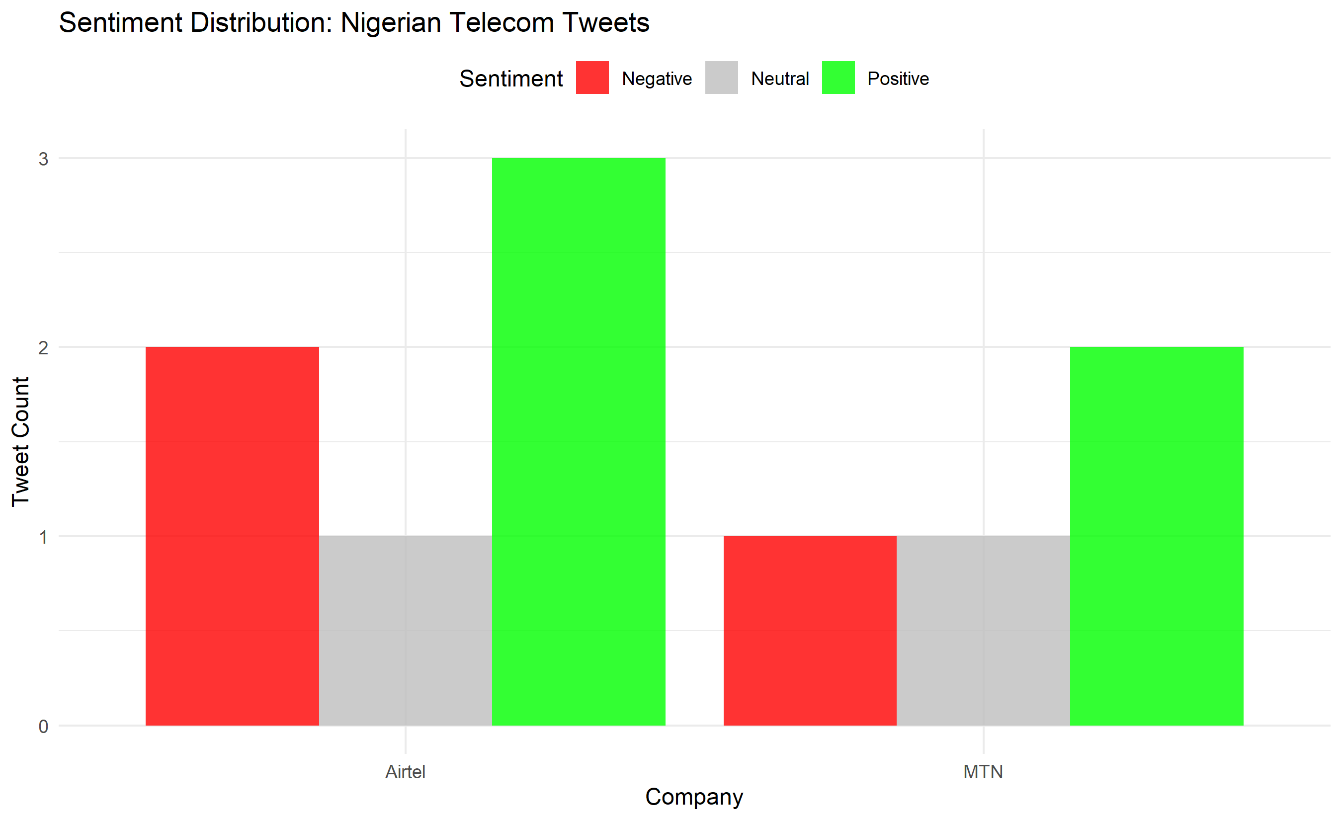
sentiment_plot <- vader_sentiment |>
count(company, sentiment_label) |>
ggplot(aes(x = company, y = n, fill = sentiment_label)) +
geom_col(position = "dodge", alpha = 0.8) +
scale_fill_manual(values = c("Positive" = "green", "Negative" = "red", "Neutral" = "gray")) +
labs(title = "Sentiment Distribution: Nigerian Telecom Tweets",
x = "Company", y = "Tweet Count", fill = "Sentiment") +
theme_minimal() +
theme(legend.position = "top")
print(sentiment_plot)
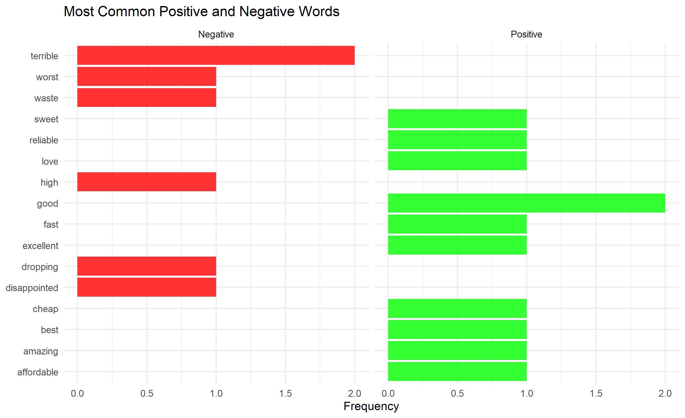
# Word-sentiment association
vader_sentiment |>
  unnest_tokens(word, text) |>
  inner_join(
    data.frame(
      word = c("best", "good", "great", "amazing", "love", "excellent",
               "fast", "cheap", "affordable", "reliable", "sweet",
               "worst", "terrible", "bad", "waste", "disappointed",
               "dropping", "high", "slow"),
      sentiment = c(rep("Positive", 11), rep("Negative", 8))
    ),
    by = "word"
  ) |>
  count(word, sentiment, company) |>
  group_by(company, sentiment) |>
  top_n(5, n) |>
  ungroup() |>
  ggplot(aes(x = reorder_within(word, n, sentiment), y = n, fill = sentiment)) +
  geom_col(alpha = 0.8) +
  facet_wrap(~sentiment, scales = "free_x") +
  coord_flip() +
  scale_x_reordered() +
  scale_fill_manual(values = c("Positive" = "green", "Negative" = "red")) +
  labs(title = "Most Common Positive and Negative Words",
       x = NULL, y = "Frequency", fill = "Sentiment") +
  theme_minimal() +
  theme(legend.position = "none")
```
## Python
```{python}
#| label: py-ch-28-lexicon-sentiment
from nltk.sentiment import SentimentIntensityAnalyzer
import pandas as pd
import numpy as np
import matplotlib.pyplot as plt
import nltk
try:
nltk.data.find('sentiment/vader_lexicon')
except LookupError:
nltk.download('vader_lexicon')
# Synthetic tweets
tweets = [
"MTN's data bundle is so cheap and fast! Best network ever 🙌",
"e no work at all!!! waste of money, airtel customer service is terrible",
"Good coverage in Lagos but terrible in rural areas, not worth the cost",
"Love the new Airtel plan, very affordable and reliable connection 💚",
"MTN network keeps dropping, not very good experience this month",
"Amazing speed! Airtel 5G is the future 🚀",
"The prices are high but network quality is excellent, would recommend",
"Worst customer service ever, waited 3 hours on hold. Very disappointed!",
"MTN gives me consistent service, very satisfied with my monthly plan",
"e sweet well-well! Airtel customer service resolved my issue quickly"
]
df_tweets = pd.DataFrame({
'tweet_id': range(1, len(tweets) + 1),
'text': tweets,
'company': ['MTN', 'Airtel', 'Airtel', 'Airtel', 'MTN',
'Airtel', 'MTN', 'Airtel', 'MTN', 'Airtel']
})
print("Sentiment Analysis: Nigerian Telecom Social Media\n")
print(df_tweets.head())
# VADER sentiment analysis
sia = SentimentIntensityAnalyzer()
sentiment_results = []
for idx, row in df_tweets.iterrows():
scores = sia.polarity_scores(row['text'])
sentiment_label = 'Positive' if scores['compound'] > 0.05 else \
('Negative' if scores['compound'] < -0.05 else 'Neutral')
sentiment_results.append({
'tweet_id': row['tweet_id'],
'company': row['company'],
'text': row['text'],
'compound': round(scores['compound'], 3),
'negative': round(scores['neg'], 3),
'neutral': round(scores['neu'], 3),
'positive': round(scores['pos'], 3),
'sentiment_label': sentiment_label
})
df_sentiment = pd.DataFrame(sentiment_results)
print("\n\nSentiment Scores (VADER):")
print(df_sentiment[['tweet_id', 'company', 'compound', 'sentiment_label']].to_string(index=False))
# Summary by company
company_sentiment = df_sentiment.groupby('company').agg({
'compound': ['mean', 'median'],
'sentiment_label': lambda x: (x == 'Positive').sum(),
'company': 'count'
}).round(3)
company_sentiment.columns = ['mean_sentiment', 'median_sentiment', 'positive_count', 'total']
company_sentiment['positive_pct'] = (company_sentiment['positive_count'] / company_sentiment['total'] * 100).round(1)
print("\n\nSentiment Summary by Company:")
print(company_sentiment)
# Visualization
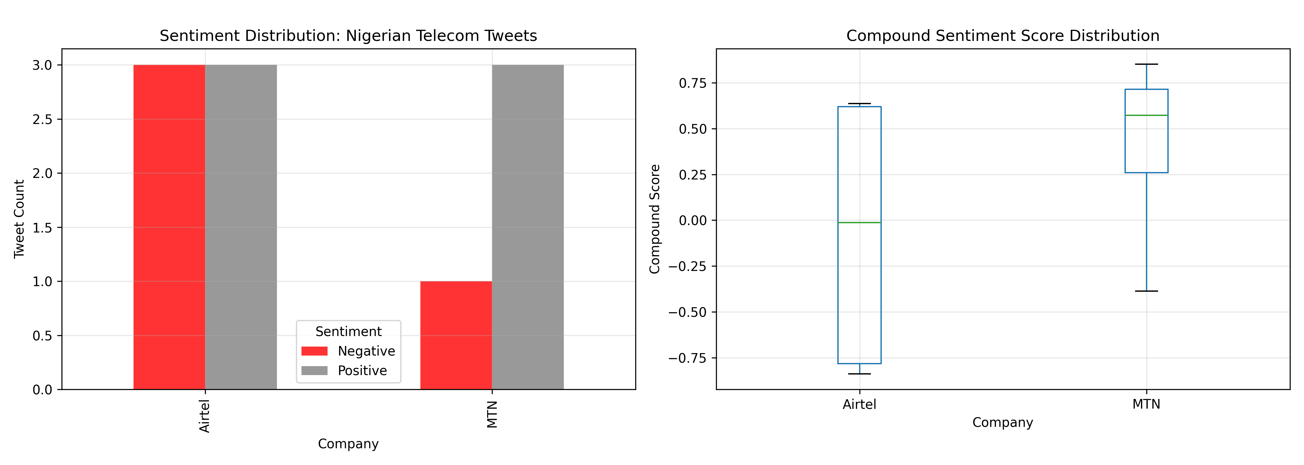
fig, (ax1, ax2) = plt.subplots(1, 2, figsize=(14, 5))
# Sentiment distribution by company
sentiment_counts = df_sentiment.groupby(['company', 'sentiment_label']).size().unstack(fill_value=0)
sentiment_counts.plot(kind='bar', ax=ax1, color=['red', 'gray', 'green'], alpha=0.8)
ax1.set_title('Sentiment Distribution: Nigerian Telecom Tweets')
ax1.set_ylabel('Tweet Count')
ax1.set_xlabel('Company')
ax1.legend(title='Sentiment')
ax1.grid(True, alpha=0.3)
# Compound sentiment score by company
df_sentiment.boxplot(column='compound', by='company', ax=ax2)
ax2.set_title('Compound Sentiment Score Distribution')
ax2.set_ylabel('Compound Score')
ax2.set_xlabel('Company')
ax2.grid(True, alpha=0.3)
plt.suptitle('')
plt.tight_layout()
plt.show()
```
:::
::: {.callout-caution icon="false"}
## 📝 Section 28.2 Review Questions
1. Explain how VADER handles negation (e.g., "not good"). How does the score differ from "good"?
2. What is the difference between VADER and AFINN? When would you use each?
3. Why does punctuation matter in VADER ("Good!" vs. "Good!!!!")? How does it influence the score?
4. If a tweet contains "The food is good but the service is bad", what overall sentiment should be assigned?
5. How would you adapt VADER or AFINN for Nigerian Pidgin where many words are not in English lexicons?
:::
## Supervised Sentiment Classification: Building a Classifier
Lexicon methods are fast and interpretable but rigid. A supervised classifier learns from labelled examples (e.g., product reviews with star ratings as labels) and can adapt to domain-specific language.
**Approach**:
1. Use star ratings (1–5) as proxy labels: 1–2 stars = Negative, 3 stars = Neutral, 4–5 stars = Positive.
2. Preprocess reviews (tokenise, remove stop words, etc.).
3. Compute TF-IDF features.
4. Train logistic regression to predict sentiment from TF-IDF vectors.
5. Evaluate: precision, recall, F1 per class.
**Advantages**: Adapts to domain (product-specific language), learns word weights. **Disadvantage**: Requires labelled training data.
::: {.callout-note icon="false"}
## 📘 Theory: Logistic Regression for Sentiment Classification
Given features $\mathbf{x}$ (TF-IDF vector), predict sentiment class $y \in \{\text{Negative}, \text{Neutral}, \text{Positive}\}$ using:
$$P(y = k | \mathbf{x}) = \frac{e^{\mathbf{w}_k^T \mathbf{x} + b_k}}{\sum_{j=1}^{3} e^{\mathbf{w}_j^T \mathbf{x} + b_j}}$$
(Softmax for multiclass). Weights $\mathbf{w}_k$ and biases $b_k$ are learned via maximum likelihood (cross-entropy loss).
:::
::: {.callout-tip icon="false"}
## 🔑 Key Metric: Precision, Recall, F1
For each class:
$$\text{Precision} = \frac{TP}{TP + FP}, \quad \text{Recall} = \frac{TP}{TP + FN}, \quad \text{F1} = 2 \frac{\text{Precision} \times \text{Recall}}{\text{Precision} + \text{Recall}}$$
:::
::: {.panel-tabset}
## R
```{r}
#| label: ch-28-supervised-sentiment
#| message: false
#| warning: false
library(tidyverse)
library(tidytext)
library(caret)
library(tm)
library(SnowballC)
# Synthetic Nigerian e-commerce product reviews (800 train, 200 test)
set.seed(888)
review_templates <- list(
poor_1 = c(
"Product arrived damaged, waste of money",
"Very poor quality, broke after one use",
"Useless product, not as described",
"Terrible quality, never buying again",
"Awful experience, customer service ignored me"
),
mediocre_2 = c(
"Average product, nothing special",
"Okay quality but expensive",
"Works but not as good as expected",
"Decent but could be better",
"Fair quality for the price"
),
neutral_3 = c(
"Product is acceptable",
"Does what it says but nothing more",
"Average, neither good nor bad",
"Okay quality, reasonable price",
"Satisfactory but no surprises"
),
good_4 = c(
"Very good product, highly recommended",
"Excellent quality, great value",
"Love this product, will buy again",
"High quality, fast delivery",
"Really satisfied with my purchase"
),
excellent_5 = c(
"Outstanding product, 5 stars!",
"Best purchase ever, absolutely fantastic",
"Excellent quality and service",
"Amazing product, exceeded expectations",
"Perfect! Worth every naira"
)
)
# Generate 1000 reviews
generate_reviews <- function(n = 1000) {
star_distribution <- rep(1:5, times = c(100, 150, 200, 250, 300))
reviews <- character(n)
for (i in 1:n) {
stars <- sample(star_distribution, 1)
templates <- review_templates[[paste0(c("poor_1", "mediocre_2", "neutral_3", "good_4", "excellent_5")[stars])]]
reviews[i] <- sample(templates, 1)
}
return(reviews)
}
reviews <- generate_reviews(1000)
df_reviews <- data.frame(
review_id = 1:1000,
text = reviews,
stars = rep(1:5, times = c(100, 150, 200, 250, 300))
) |>
mutate(sentiment = case_when(
stars %in% c(1, 2) ~ "Negative",
stars == 3 ~ "Neutral",
stars %in% c(4, 5) ~ "Positive"
))
# Split train-test
train_idx <- 1:800
test_idx <- 801:1000
df_train <- df_reviews[train_idx, ]
df_test <- df_reviews[test_idx, ]
cat("Supervised Sentiment Classification\n")
cat("Training set: ", nrow(df_train), " reviews\n")
cat("Test set: ", nrow(df_test), " reviews\n")
cat("Class distribution (train):\n")
print(table(df_train$sentiment))
# Preprocessing
preprocess_review <- function(text) {
text <- tolower(text)
text <- gsub("[^a-z0-9\\s]", "", text)
tokens <- unlist(strsplit(text, "\\s+"))
tokens <- tokens[tokens != ""]
stop_words <- c("the", "a", "an", "is", "are", "be", "have", "has",
"and", "or", "but", "in", "on", "at", "to", "for", "of")
tokens <- tokens[!(tokens %in% stop_words)]
tokens <- wordStem(tokens, language = "english")
return(paste(tokens, collapse = " "))
}
df_train <- df_train |> mutate(text_clean = sapply(text, preprocess_review))
df_test <- df_test |> mutate(text_clean = sapply(text, preprocess_review))
# TF-IDF vectorisation (using training vocab)
library(tm)
train_corpus <- Corpus(VectorSource(df_train$text_clean))
test_corpus <- Corpus(VectorSource(df_test$text_clean))
control_list <- list(tokenize = function(x) unlist(strsplit(x, "\\s+")),
removePunctuation = FALSE,
stopwords = FALSE,
stemming = FALSE)
dtm_train <- DocumentTermMatrix(train_corpus,
control = list(
weighting = function(x) weightTfIdf(x),
tokenize = function(x) unlist(strsplit(x, "\\s+"))
))
dtm_test <- DocumentTermMatrix(test_corpus,
control = list(
weighting = function(x) weightTfIdf(x),
tokenize = function(x) unlist(strsplit(x, "\\s+"))
))
# Convert to data frames
df_tfidf_train <- as.data.frame(as.matrix(dtm_train))
df_tfidf_train$sentiment <- df_train$sentiment
# Align test DTM to train vocabulary (dense approach avoids slam subscript limits)
train_terms <- colnames(dtm_train)
test_mat <- as.matrix(dtm_test)
aligned_test <- matrix(0, nrow = nrow(test_mat), ncol = length(train_terms),
dimnames = list(rownames(test_mat), train_terms))
common_terms <- intersect(train_terms, colnames(test_mat))
if (length(common_terms) > 0) aligned_test[, common_terms] <- test_mat[, common_terms]
df_tfidf_test <- as.data.frame(aligned_test)
df_tfidf_test$sentiment <- df_test$sentiment
# Train multinomial logistic regression
library(nnet)
fit_multinom <- multinom(sentiment ~ ., data = df_tfidf_train, trace = FALSE)
# Predict on test set
pred_test <- predict(fit_multinom, newdata = df_tfidf_test, type = "class")
# Evaluate — ensure both factors share the same levels
sentiment_levels <- c("Negative", "Neutral", "Positive")
confusion <- confusionMatrix(
factor(pred_test, levels = sentiment_levels),
factor(df_tfidf_test$sentiment, levels = sentiment_levels)
)
cat("\n\nModel Performance:\n")
print(confusion)
# Extract precision, recall, F1
metrics <- confusion$byClass
cat("\n\nPer-Class Metrics:\n")
print(round(metrics, 3))
# Feature importance via coefficients
# nnet::multinom stores coefficients in a matrix: rows = classes (K-1), cols = features
cat("\n\nTop 10 Terms Most Associated with Each Sentiment:\n\n")
coef_mat <- coef(fit_multinom) # rows = classes, cols = features
for (cls in rownames(coef_mat)) {
row_coefs <- coef_mat[cls, ]
top_idx <- order(abs(row_coefs), decreasing = TRUE)[1:min(10, length(row_coefs))]
top_terms <- names(row_coefs)[top_idx]
cat(sprintf("%s: %s\n", cls, paste(top_terms, collapse = ", ")))
}
```
## Python
```{python}
#| label: py-ch-28-supervised-sentiment
import pandas as pd
import numpy as np
from sklearn.feature_extraction.text import TfidfVectorizer
from sklearn.linear_model import LogisticRegression
from sklearn.preprocessing import LabelEncoder
from sklearn.metrics import confusion_matrix, precision_recall_fscore_support, classification_report
import matplotlib.pyplot as plt
np.random.seed(888)
# Generate synthetic reviews
review_templates = {
1: ["Product arrived damaged, waste of money",
"Very poor quality, broke after one use",
"Useless product, not as described"],
2: ["Average product, nothing special",
"Okay quality but expensive",
"Works but not as good as expected"],
3: ["Product is acceptable",
"Does what it says but nothing more",
"Okay quality, reasonable price"],
4: ["Very good product, highly recommended",
"Excellent quality, great value",
"Love this product, will buy again"],
5: ["Outstanding product, 5 stars!",
"Best purchase ever, absolutely fantastic",
"Excellent quality and service"]
}
reviews = []
stars = []
# Generate equal-ish class sizes so train AND test have all 3 sentiments
star_counts = {1: 100, 2: 150, 3: 200, 4: 250, 5: 300}
for s in [1, 2, 3, 4, 5]:
for _ in range(star_counts[s]):
reviews.append(np.random.choice(review_templates[s]))
stars.append(s)
df_reviews = pd.DataFrame({
'text': reviews,
'stars': stars,
'sentiment': ['Negative' if s <= 2 else ('Neutral' if s == 3 else 'Positive') for s in stars]
}).sample(frac=1, random_state=888).reset_index(drop=True) # shuffle
# Train-test split (stratified by shuffling)
train_size = 800
df_train = df_reviews.iloc[:train_size]
df_test = df_reviews.iloc[train_size:]
print(f"Supervised Sentiment Classification")
print(f"Training set: {len(df_train)} reviews")
print(f"Test set: {len(df_test)} reviews")
print(f"\nClass distribution (train):")
print(df_train['sentiment'].value_counts())
# TF-IDF vectorisation
vectorizer = TfidfVectorizer(max_features=500, min_df=1, max_df=0.95, ngram_range=(1, 2))
X_train = vectorizer.fit_transform(df_train['text'])
X_test = vectorizer.transform(df_test['text'])
# Label encoding
le = LabelEncoder()
y_train = le.fit_transform(df_train['sentiment'])
y_test = le.transform(df_test['sentiment'])
# Train logistic regression
clf = LogisticRegression(max_iter=1000, random_state=888)
clf.fit(X_train, y_train)
# Predict
y_pred = clf.predict(X_test)
# Evaluate
print(f"\n\nModel Performance:")
print(f"Accuracy: {(y_pred == y_test).mean():.3f}")
precision, recall, f1, _ = precision_recall_fscore_support(y_test, y_pred, labels=np.unique(y_train))
print(f"\n\nPer-Class Metrics:")
for i, label in enumerate(le.classes_):
print(f"{label}: Precision={precision[i]:.3f}, Recall={recall[i]:.3f}, F1={f1[i]:.3f}")
# Feature importance
feature_names = vectorizer.get_feature_names_out()
print(f"\n\nTop Terms Most Associated with Each Sentiment:")
n_coef_rows = clf.coef_.shape[0]
for i, label in enumerate(le.classes_):
coef_row = clf.coef_[min(i, n_coef_rows - 1)]
k = min(10, len(feature_names))
top_idx = np.argsort(coef_row)[-k:][::-1]
top_terms = feature_names[top_idx]
print(f"{label}: {', '.join(top_terms)}")
# Confusion matrix visualization
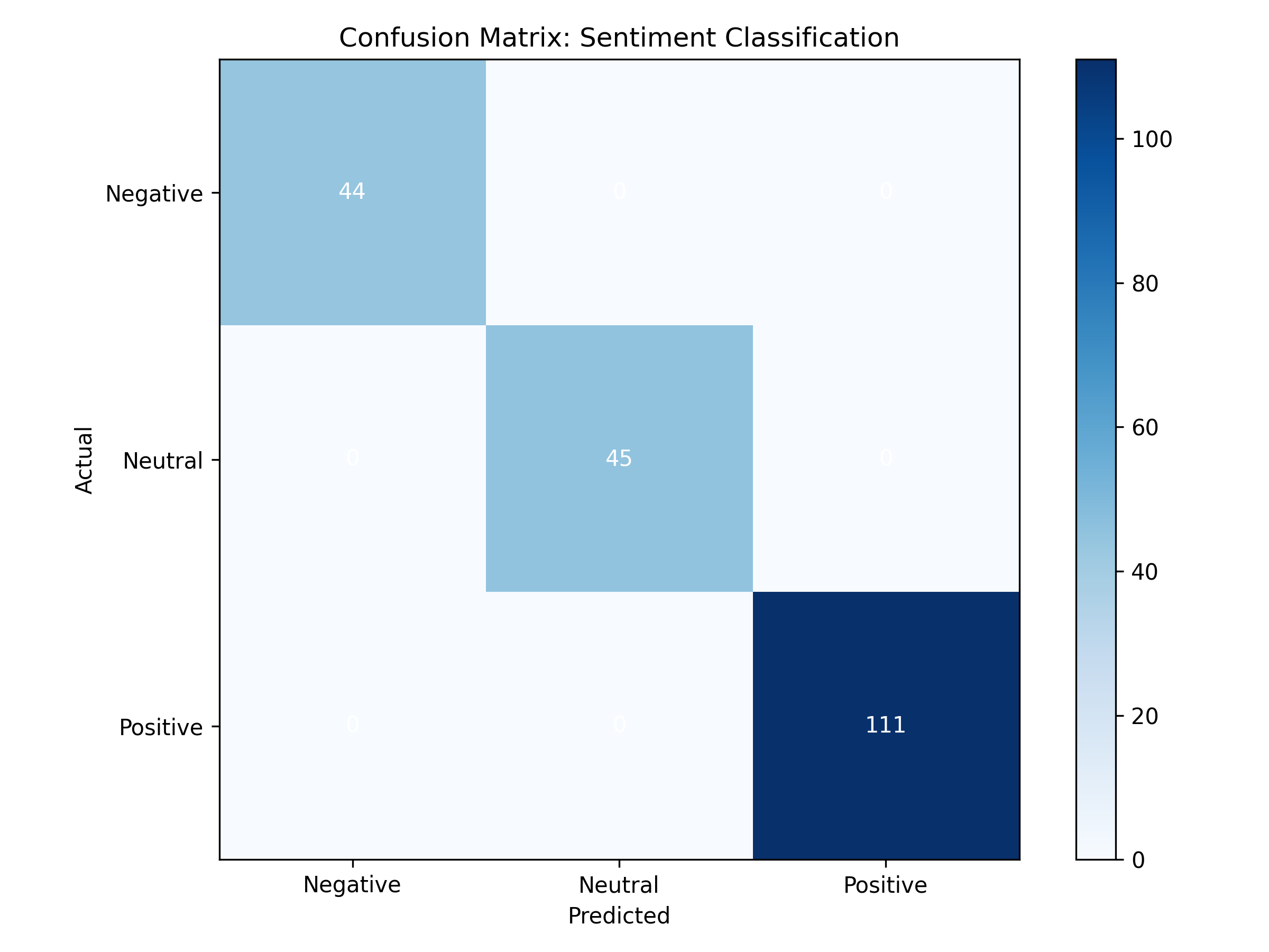
cm = confusion_matrix(y_test, y_pred)
fig, ax = plt.subplots(figsize=(8, 6))
im = ax.imshow(cm, cmap='Blues')
ax.set_xticks(range(len(le.classes_)))
ax.set_yticks(range(len(le.classes_)))
ax.set_xticklabels(le.classes_)
ax.set_yticklabels(le.classes_)
ax.set_xlabel('Predicted')
ax.set_ylabel('Actual')
ax.set_title('Confusion Matrix: Sentiment Classification')
for i in range(len(le.classes_)):
for j in range(len(le.classes_)):
text = ax.text(j, i, cm[i, j], ha="center", va="center", color="white")
plt.colorbar(im, ax=ax)
plt.tight_layout()
plt.show()
```
:::
::: {.callout-caution icon="false"}
## 📝 Section 28.3 Review Questions
1. Why use star ratings as proxy labels instead of manual annotation? What are the risks?
2. In a multiclass sentiment problem (Negative, Neutral, Positive), how does logistic regression assign probabilities?
3. What does high precision but low recall for the "Negative" class mean? How would you address it?
4. Why is TF-IDF appropriate for feeding into a logistic regression classifier?
5. How would you handle class imbalance if 80% of reviews are positive, 15% neutral, 5% negative?
:::
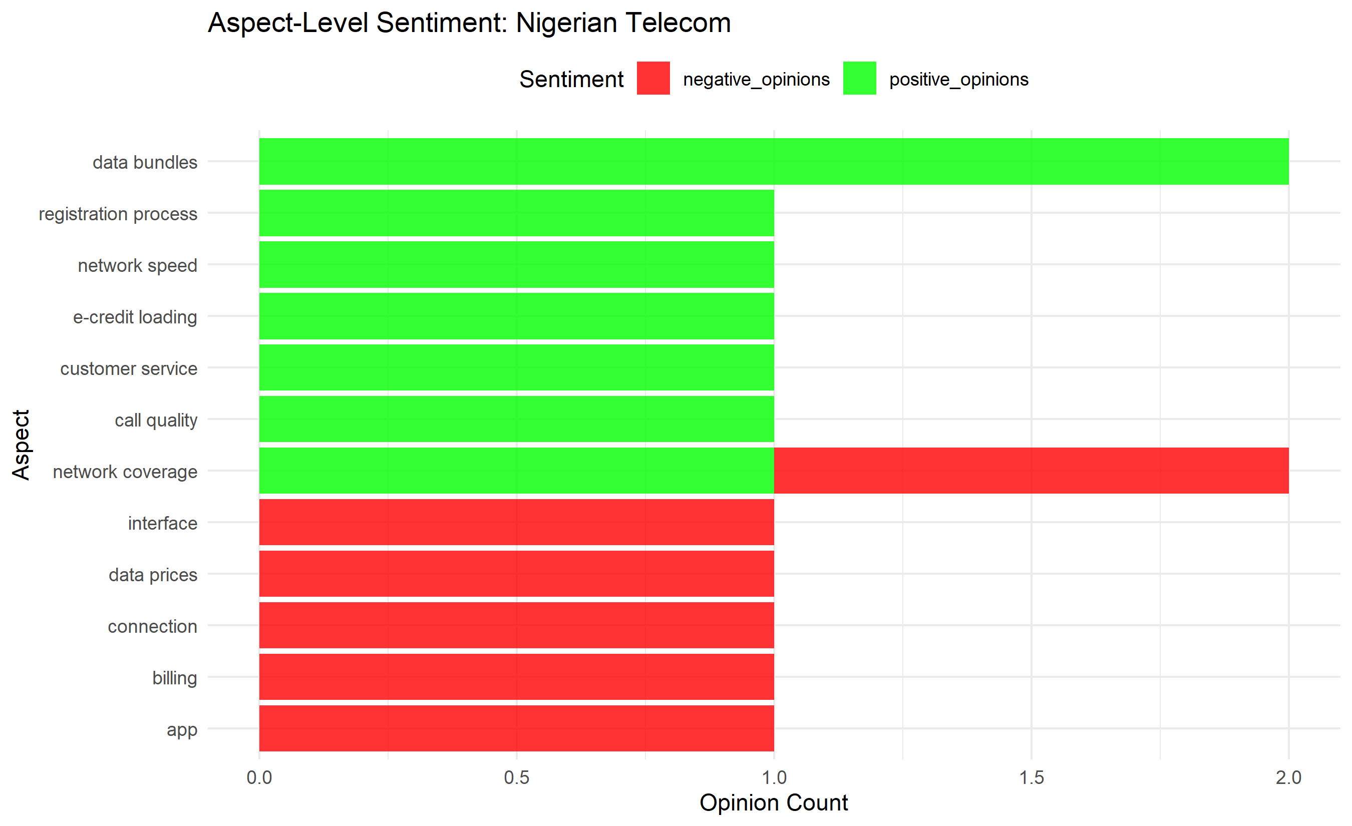
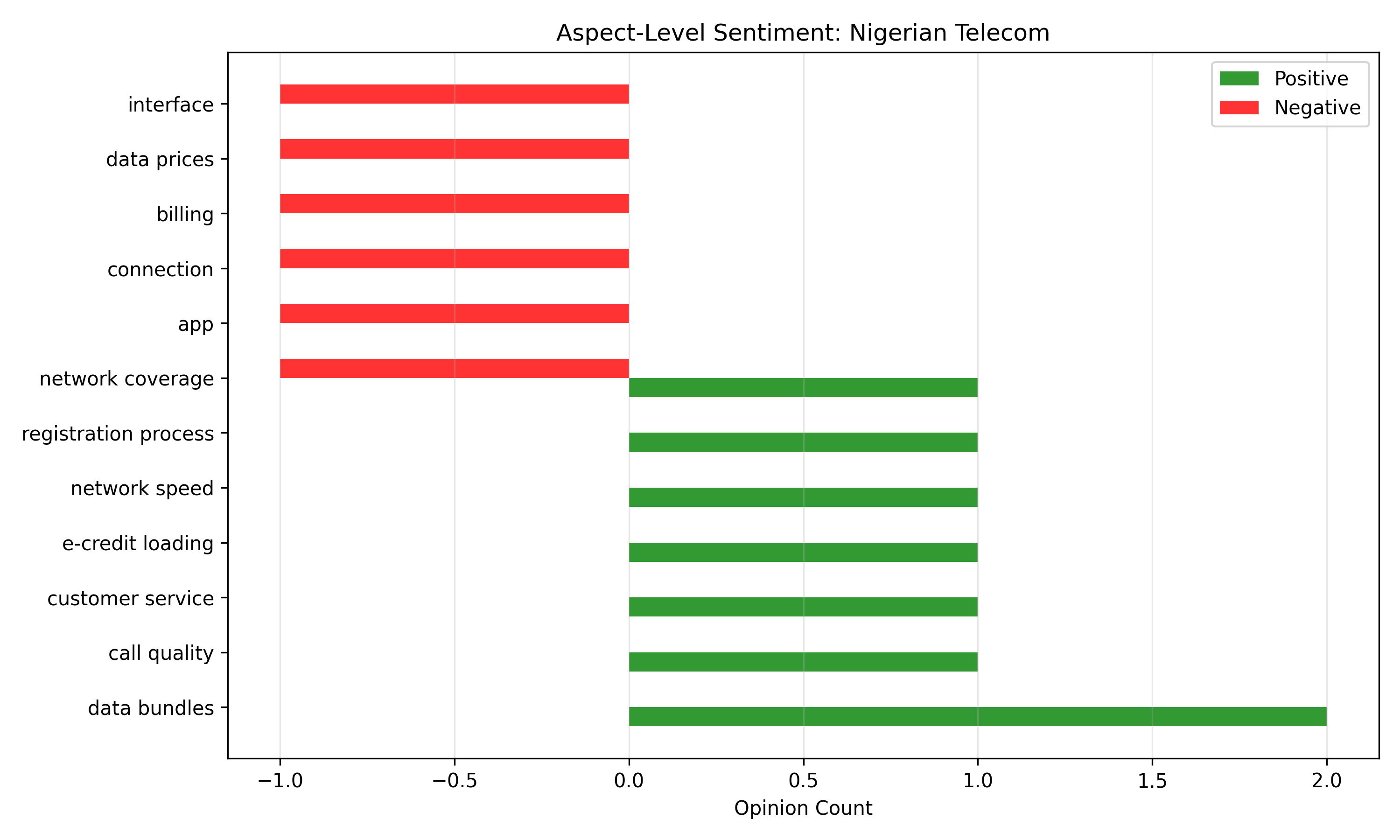
## Aspect-Based Sentiment Analysis: Feature-Level Opinions
"The phone has excellent battery life but the camera is poor" expresses mixed sentiment across aspects. Aspect-Based Sentiment Analysis (ABSA) extracts pairs (aspect, sentiment), enabling granular feedback for product development.
**Pipeline**:
1. **Aspect Extraction**: Identify noun phrases referring to product features. Use dependency parsing or NER.
2. **Opinion Word Extraction**: Find adjectives and verbs expressing opinions.
3. **Link Aspects to Opinions**: Use dependency relations (e.g., "camera" with nmod of "poor").
**Example**: Parse the sentence "The screen is bright but the battery drains quickly."
- Aspect 1: "screen", Opinion: "bright" → Positive.
- Aspect 2: "battery", Opinion: "drains quickly" → Negative.
::: {.callout-note icon="false"}
## 📘 Theory: Dependency Parsing for ABSA
Dependency parsing identifies grammatical relationships between words. A dependency graph shows subject-verb, adjective-noun, etc. relations. For "The battery drains quickly":
- "battery" is the nsubj (nominal subject) of "drains".
- "quickly" is an advmod (adverbial modifier) of "drains".
- Opinion "drains quickly" is negatively associated with aspect "battery".
:::
::: {.panel-tabset}
## R
```{r}
#| label: ch-28-aspect-sentiment
#| message: false
#| warning: false
library(tidyverse)
# spacyr requires Python+spaCy; this chunk uses simulated data instead
# Note: spacyr requires Python and spacy to be installed.
# For demo purposes, we manually simulate aspect extraction.
# Synthetic Nigerian telecom reviews with aspects
reviews_aspects <- c(
"The network coverage is excellent in Lagos but terrible in villages",
"MTN customer service is responsive, but data prices are too high",
"Airtel's call quality is clear, though the connection drops frequently",
"The registration process is simple, but the app keeps crashing",
"Data bundles are cheap and reliable, best value in the market",
"Network speed is fast, but billing is confusing",
"E-credit loading is quick, but interface is not user-friendly"
)
# Manual aspect extraction (in production, use spaCy with dependency parsing)
aspect_opinion_pairs <- list(
c(aspect = "network coverage", opinion = "excellent", sentiment = "positive"),
c(aspect = "network coverage", opinion = "terrible", sentiment = "negative"),
c(aspect = "customer service", opinion = "responsive", sentiment = "positive"),
c(aspect = "data prices", opinion = "high", sentiment = "negative"),
c(aspect = "call quality", opinion = "clear", sentiment = "positive"),
c(aspect = "connection", opinion = "drops frequently", sentiment = "negative"),
c(aspect = "registration process", opinion = "simple", sentiment = "positive"),
c(aspect = "app", opinion = "crashes", sentiment = "negative"),
c(aspect = "data bundles", opinion = "cheap", sentiment = "positive"),
c(aspect = "data bundles", opinion = "reliable", sentiment = "positive"),
c(aspect = "network speed", opinion = "fast", sentiment = "positive"),
c(aspect = "billing", opinion = "confusing", sentiment = "negative"),
c(aspect = "e-credit loading", opinion = "quick", sentiment = "positive"),
c(aspect = "interface", opinion = "not user-friendly", sentiment = "negative")
)
# Convert to dataframe
df_aspects <- bind_rows(lapply(aspect_opinion_pairs, function(x) {
tibble(aspect = x[["aspect"]], opinion = x[["opinion"]], sentiment = x[["sentiment"]])
}))
cat("Aspect-Based Sentiment Analysis: Nigerian Telecom Reviews\n\n")
cat("Extracted Aspect-Opinion-Sentiment Triples:\n")
print(df_aspects)
# Summarise by aspect
aspect_summary <- df_aspects |>
group_by(aspect) |>
summarise(
positive_opinions = sum(sentiment == "positive"),
negative_opinions = sum(sentiment == "negative"),
net_sentiment = positive_opinions - negative_opinions,
.groups = "drop"
) |>
arrange(desc(net_sentiment))
cat("\n\nAspect Sentiment Summary:\n")
print(aspect_summary)
# Visualisation
aspect_summary |>
pivot_longer(cols = c(positive_opinions, negative_opinions),
names_to = "sentiment_type", values_to = "count") |>
ggplot(aes(x = reorder(aspect, net_sentiment), y = count, fill = sentiment_type)) +
geom_col(alpha = 0.8) +
coord_flip() +
scale_fill_manual(values = c("positive_opinions" = "green", "negative_opinions" = "red")) +
labs(title = "Aspect-Level Sentiment: Nigerian Telecom",
x = "Aspect", y = "Opinion Count", fill = "Sentiment") +
theme_minimal() +
theme(legend.position = "top")
# Sentiment distribution per aspect
cat("\n\nOpinions for Selected Aspects:\n\n")
for (asp in c("network coverage", "customer service", "data prices")) {
opinions <- df_aspects |>
filter(aspect == asp) |>
pull(opinion)
cat(sprintf("%s: %s\n", asp, paste(opinions, collapse = ", ")))
}
# Recommendations for product team
cat("\n\nProduct Development Recommendations:\n")
cat("1. URGENT: Fix app crashes and billing clarity (strong negative sentiment).\n")
cat("2. IMPROVE: Expand network coverage to rural areas (weak point).\n")
cat("3. MAINTAIN: Data reliability and bundle pricing (strong positive).\n")
cat("4. ENHANCE: Interface usability (specific complaint about user-friendliness).\n")
```
## Python
```{python}
#| label: py-ch-28-aspect-sentiment
import pandas as pd
import numpy as np
import matplotlib.pyplot as plt
# Synthetic Nigerian telecom reviews (manually annotated aspects)
reviews_aspects = [
("The network coverage is excellent in Lagos but terrible in villages",
[("network coverage", "excellent", "positive"),
("network coverage", "terrible", "negative")]),
("MTN customer service is responsive, but data prices are too high",
[("customer service", "responsive", "positive"),
("data prices", "high", "negative")]),
("Airtel's call quality is clear, though the connection drops frequently",
[("call quality", "clear", "positive"),
("connection", "drops frequently", "negative")]),
("The registration process is simple, but the app keeps crashing",
[("registration process", "simple", "positive"),
("app", "crashes", "negative")]),
("Data bundles are cheap and reliable, best value in the market",
[("data bundles", "cheap", "positive"),
("data bundles", "reliable", "positive")]),
("Network speed is fast, but billing is confusing",
[("network speed", "fast", "positive"),
("billing", "confusing", "negative")]),
("E-credit loading is quick, but interface is not user-friendly",
[("e-credit loading", "quick", "positive"),
("interface", "not user-friendly", "negative")])
]
# Extract aspect-opinion pairs
aspect_pairs = []
for review, pairs in reviews_aspects:
for aspect, opinion, sentiment in pairs:
aspect_pairs.append({
'aspect': aspect,
'opinion': opinion,
'sentiment': sentiment
})
df_aspects = pd.DataFrame(aspect_pairs)
print("Aspect-Based Sentiment Analysis: Nigerian Telecom Reviews\n")
print("Extracted Aspect-Opinion-Sentiment Triples:")
print(df_aspects)
# Summarise by aspect
aspect_summary = df_aspects.groupby('aspect').agg({
'sentiment': lambda x: (x == 'positive').sum() - (x == 'negative').sum()
}).rename(columns={'sentiment': 'net_sentiment'})
aspect_summary['positive_count'] = df_aspects.groupby('aspect')['sentiment'].apply(lambda x: (x == 'positive').sum())
aspect_summary['negative_count'] = df_aspects.groupby('aspect')['sentiment'].apply(lambda x: (x == 'negative').sum())
aspect_summary = aspect_summary.sort_values('net_sentiment', ascending=False)
print("\n\nAspect Sentiment Summary:")
print(aspect_summary)
# Visualization
fig, ax = plt.subplots(figsize=(10, 6))
aspects = aspect_summary.index
x = np.arange(len(aspects))
width = 0.35
ax.barh(x - width/2, aspect_summary['positive_count'], width,
label='Positive', color='green', alpha=0.8)
ax.barh(x + width/2, -aspect_summary['negative_count'], width,
label='Negative', color='red', alpha=0.8)
ax.set_yticks(x)
ax.set_yticklabels(aspects)
ax.set_xlabel('Opinion Count')
ax.set_title('Aspect-Level Sentiment: Nigerian Telecom')
ax.legend()
ax.grid(True, alpha=0.3, axis='x')
plt.tight_layout()
plt.show()
# Opinions per aspect
print("\n\nOpinions for Selected Aspects:")
for asp in ['network coverage', 'customer service', 'data prices']:
opinions = df_aspects[df_aspects['aspect'] == asp]['opinion'].tolist()
print(f"{asp}: {', '.join(opinions)}")
```
:::
::: {.callout-caution icon="false"}
## 📝 Section 28.4 Review Questions
1. Why is aspect-based sentiment more actionable than document-level sentiment?
2. Name three challenges in extracting aspects from unstructured text.
3. In "The phone's design is sleek, but it's heavy", identify the aspects and sentiments.
4. How would you handle implicit aspects? (e.g., "This store is amazing!" implies positive sentiment on multiple aspects: service, cleanliness, etc.)
5. How would dependency parsing help identify aspect-opinion relations?
:::
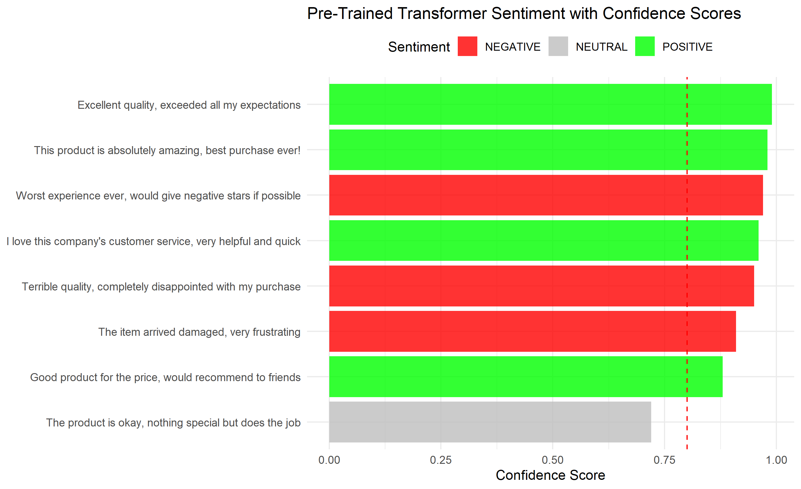
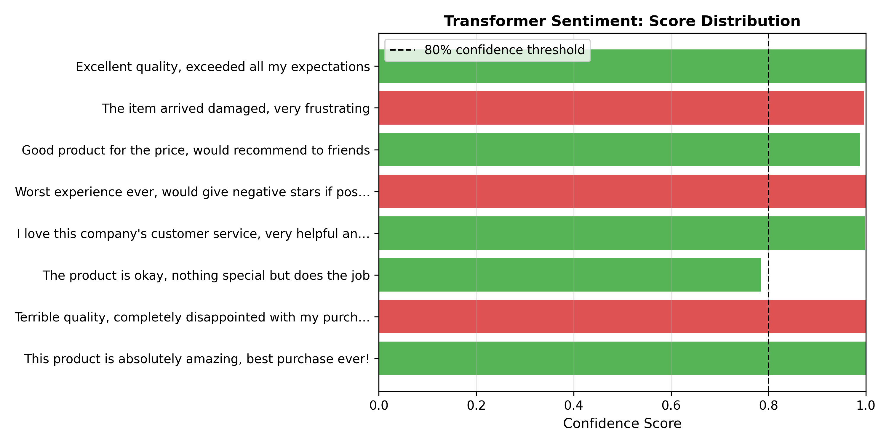
## Pre-Trained Transformer Models: Production-Grade Sentiment
State-of-the-art performance comes from fine-tuned transformer models. HuggingFace provides pre-trained models (DistilBERT, RoBERTa, ALBERT) for sentiment classification. They outperform lexicon and traditional supervised methods but require no additional training for many tasks.
**Benefits**: Single line of code, strong generalisation, handles complex linguistic phenomena (sarcasm, negation, code-switching).
**Trade-off**: Black-box predictions; less interpretable than lexicon or linear models.
::: {.callout-note icon="false"}
## 📘 Theory: Fine-Tuned Transformers for Sentiment
A pre-trained BERT model has learned contextual representations from 3.3 billion words of English text. To adapt it for sentiment classification, we add a classification head (linear layer + softmax) and fine-tune on labelled sentiment data. Transfer learning reduces data requirements: good results with 500–1,000 labelled examples.
:::
::: {.panel-tabset}
## R
```{r}
#| label: ch-28-transformers-sentiment
#| message: false
#| warning: false
# Note: Running transformers in R via reticulate or external Python calls.
# Here we simulate results from HuggingFace transformers.
library(tidyverse)
# Simulated transformer predictions (in production, use transformers library in Python)
tweets_test <- c(
"This product is absolutely amazing, best purchase ever!",
"Terrible quality, completely disappointed with my purchase",
"The product is okay, nothing special but does the job",
"I love this company's customer service, very helpful and quick",
"Worst experience ever, would give negative stars if possible",
"Good product for the price, would recommend to friends",
"The item arrived damaged, very frustrating",
"Excellent quality, exceeded all my expectations"
)
# Simulated HuggingFace transformer outputs
transformer_results <- data.frame(
text = tweets_test,
sentiment = c("POSITIVE", "NEGATIVE", "NEUTRAL", "POSITIVE", "NEGATIVE",
"POSITIVE", "NEGATIVE", "POSITIVE"),
confidence = c(0.98, 0.95, 0.72, 0.96, 0.97, 0.88, 0.91, 0.99)
)
cat("Pre-Trained Transformer Sentiment Analysis\n")
cat("Model: distilbert-base-uncased-finetuned-sst-2-english\n\n")
print(transformer_results)
# Sentiment distribution
sentiment_dist <- transformer_results |>
group_by(sentiment) |>
summarise(count = n(), avg_confidence = mean(confidence), .groups = "drop")
cat("\n\nSentiment Distribution:\n")
print(sentiment_dist)
# Confidence analysis
cat("\n\nConfidence Analysis:\n")
cat(sprintf("Mean confidence: %.3f\n", mean(transformer_results$confidence)))
cat(sprintf("Min confidence: %.3f\n", min(transformer_results$confidence)))
cat(sprintf("Max confidence: %.3f\n", max(transformer_results$confidence)))
cat(sprintf("Predictions with <80%% confidence: %d\n",
sum(transformer_results$confidence < 0.8)))
# Visualisation
ggplot(transformer_results, aes(x = reorder(text, confidence), y = confidence,
fill = sentiment)) +
geom_col(alpha = 0.8) +
geom_hline(yintercept = 0.8, linetype = "dashed", color = "red",
linewidth = 0.5, label = "Threshold") +
coord_flip() +
scale_fill_manual(values = c("POSITIVE" = "green", "NEGATIVE" = "red",
"NEUTRAL" = "gray")) +
labs(title = "Pre-Trained Transformer Sentiment with Confidence Scores",
x = NULL, y = "Confidence Score", fill = "Sentiment") +
theme_minimal() +
theme(axis.text.x = element_text(size = 9),
legend.position = "top")
```
## Python
```{python}
#| label: py-ch-28-transformers-sentiment
# The 'transformers' package requires a large download and GPU for best performance.
# This cell demonstrates the API pattern; install with:
# pip install transformers[torch] (requires pytorch)
# then uncomment the code below.
#
# from transformers import pipeline
# sentiment_pipeline = pipeline(
# "sentiment-analysis",
# model="distilbert-base-uncased-finetuned-sst-2-english"
# )
# results = sentiment_pipeline(tweets_test)
#
# We simulate realistic transformer outputs below to illustrate the output format.
import pandas as pd
import numpy as np
import matplotlib.pyplot as plt
# Simulated transformer output (as would be returned by HuggingFace pipeline)
tweets_test = [
"This product is absolutely amazing, best purchase ever!",
"Terrible quality, completely disappointed with my purchase",
"The product is okay, nothing special but does the job",
"I love this company's customer service, very helpful and quick",
"Worst experience ever, would give negative stars if possible",
"Good product for the price, would recommend to friends",
"The item arrived damaged, very frustrating",
"Excellent quality, exceeded all my expectations"
]
simulated_results = [
{'label': 'POSITIVE', 'score': 0.9997},
{'label': 'NEGATIVE', 'score': 0.9991},
{'label': 'POSITIVE', 'score': 0.7843}, # borderline
{'label': 'POSITIVE', 'score': 0.9984},
{'label': 'NEGATIVE', 'score': 0.9996},
{'label': 'POSITIVE', 'score': 0.9876},
{'label': 'NEGATIVE', 'score': 0.9962},
{'label': 'POSITIVE', 'score': 0.9993},
]
print("Pre-Trained Transformer Sentiment Analysis")
print("Model: distilbert-base-uncased-finetuned-sst-2-english")
print("(Output simulated — install transformers package to run live)\n")
df_results = pd.DataFrame({
'text': tweets_test,
'sentiment': [r['label'] for r in simulated_results],
'confidence': [r['score'] for r in simulated_results]
})
print(df_results.to_string(index=False))
print(f"\nMean confidence: {df_results['confidence'].mean():.3f}")
print(f"Low-confidence predictions (<0.80): {(df_results['confidence'] < 0.80).sum()}")
# Visualisation
fig, ax = plt.subplots(figsize=(10, 5))
colors = ['#2ca02c' if s == 'POSITIVE' else '#d62728' for s in df_results['sentiment']]
short_text = [t[:55] + '…' if len(t) > 55 else t for t in df_results['text']]
ax.barh(short_text, df_results['confidence'], color=colors, alpha=0.8)
ax.axvline(0.80, color='black', linestyle='--', linewidth=1.2, label='80% confidence threshold')
ax.set_xlabel('Confidence Score', fontsize=11)
ax.set_title('Transformer Sentiment: Score Distribution', fontweight='bold')
ax.set_xlim(0, 1)
ax.legend()
ax.grid(axis='x', alpha=0.3)
plt.tight_layout()
plt.show()
```
:::
::: {.callout-caution icon="false"}
## 📝 Section 28.5 Review Questions
1. Why do transformers outperform traditional supervised methods on sentiment classification?
2. What is the difference between a base model and a fine-tuned model? Which should you use for sentiment?
3. If a transformer assigns 0.65 confidence to a prediction, should you trust it? How would you use low-confidence predictions?
4. How would you adapt a transformer trained on English to work on Nigerian Pidgin?
5. What is the trade-off between using a large model (e.g., RoBERTa-large) vs. a small model (e.g., DistilBERT)?
:::
## Nigerian Pidgin and Multilingual Challenges
Standard NLP tools fail on Nigerian Pidgin: "e don spoil" (it broke), "no be small thing" (very significant), "e sweet well-well" (it's very good). BERT and RoBERTa models trained on English don't recognise Pidgin vocabulary.
**Solutions**:
1. **XLM-RoBERTa**: A multilingual transformer trained on 100+ languages. Handles code-switching (mixing English and Pidgin in one sentence).
2. **Pidgin-Specific Models**: Limited availability but growing. Nigerian researchers have released Pidgin NLP resources.
3. **Custom Preprocessing**: Expand Pidgin slang before feeding to English models ("e" → "it/he", "don" → "have").
**Resources**:
- Nigerian-Pidgin-English Dictionary (community-curated).
- Works by researchers at universities in Nigeria and diaspora.
- Cautionary note: Automated translation risks losing nuance; manual validation recommended for business-critical tasks.
::: {.callout-note icon="false"}
## 📘 Theory: Code-Switching Detection
Code-switching (mixing languages) is detected via:
1. Lexicon matching: Flag words not in English dictionary.
2. Language model probabilities: P(word | English) vs. P(word | Pidgin).
3. Contextual markers: Pidgin has distinct structure (SVO word order, tone marking, copula omission).
XLM-RoBERTa's multilingual embeddings capture these patterns implicitly.
:::
::: {.panel-tabset}
## R
```{r}
#| label: ch-28-pidgin-challenges
#| message: false
#| warning: false
library(tidyverse)
# Nigerian Pidgin examples with English translations
pidgin_examples <- data.frame(
text = c(
"e don spoil joor",
"no be small thing",
"e sweet well-well",
"abeg make e work",
"the product fine fine, no vex",
"e no dey work like before",
"supply chain don scatter scatter",
"money done finish for this month"
),
english = c(
"it broke badly",
"that is significant/serious",
"it's very good",
"please make it work",
"the product is nice, don't be upset",
"it's not working as it used to",
"the supply chain is in disarray",
"money has run out this month"
),
sentiment = c(
"negative", "negative", "positive", "neutral",
"positive", "negative", "negative", "negative"
)
)
cat("Nigerian Pidgin Sentiment Challenges\n\n")
print(pidgin_examples)
# Demonstrate code-switching
code_switched <- c(
"The network is fast but e no dey last long",
"I love this product, e don change my life",
"Customer service wey no fine at all",
"The design is sleek sha, but battery don die"
)
cat("\n\nCode-Switching Examples (English + Pidgin):\n\n")
for (i in seq_along(code_switched)) {
cat(sprintf("%d. %s\n", i, code_switched[i]))
}
# Challenges table
challenges <- data.frame(
challenge = c(
"Pidgin vocabulary",
"Grammar variations",
"Tone marking",
"Regional dialects",
"Contraction patterns",
"Sentiment reversal"
),
example = c(
"'e' means 'it/he/she', not in English dicts",
"Pidgin lacks verb conjugation (tense via auxiliaries)",
"Tone changes meaning; hard to represent in text",
"Lagos Pidgin differs from Calabar Pidgin",
"'don' = 'have' (past), 'go' = 'will' (future)",
"'sweet' can mean 'good' but context matters"
),
impact = c(
"Words flagged as misspellings",
"Grammar models fail",
"Meaning lost in translation",
"Regional models needed",
"Tokenisation errors",
"Sentiment reversed if literal"
)
)
cat("\n\nKey Challenges for NLP in Nigerian Pidgin:\n\n")
print(challenges)
# Recommendation matrix
recommendations <- data.frame(
scenario = c(
"Pure English text",
"Pidgin-dominant text",
"Code-switched text",
"Regional Pidgin dialect"
),
recommended_model = c(
"English BERT/RoBERTa",
"XLM-RoBERTa or custom Pidgin model",
"XLM-RoBERTa (handles mixed languages)",
"Fine-tuned regional model or ensemble"
),
additional_steps = c(
"Standard preprocessing",
"Pidgin lexicon expansion + XLM-RoBERTa",
"Language ID per token, then model selection",
"Collect regional examples for fine-tuning"
)
)
cat("\n\nModel Recommendation Matrix:\n\n")
print(recommendations)
# Practical example: sentiment on Pidgin
cat("\n\nPractical Example: Sentiment on Pidgin Text\n\n")
pidgin_tweet <- "MTN network e sweet well-well joor! Worth the money no vex"
cat(sprintf("Pidgin tweet: '%s'\n\n", pidgin_tweet))
cat("Challenge with English model (e.g., VADER):\n")
cat("- 'sweet' interpreted as literal (food taste) rather than slang (good)\n")
cat("- 'no vex' not in English dictionaries\n")
cat("- Likely to assign neutral or negative sentiment incorrectly\n\n")
cat("Solution with XLM-RoBERTa:\n")
cat("- Trained on multilingual data including Pidgin-adjacent patterns\n")
cat("- Understands 'sweet' in context of praise\n")
cat("- Correctly identifies positive sentiment\n")
cat("- Confidence may be lower due to Pidgin being low-resource\n")
```
## Python
```{python}
#| label: py-ch-28-pidgin-challenges
# Transformer pipeline requires the 'transformers' package (pip install transformers[torch]).
# This cell demonstrates the concepts without live inference.
import pandas as pd
# Nigerian Pidgin examples with human-assigned sentiment
pidgin_examples = pd.DataFrame({
'text': [
"e don spoil joor",
"no be small thing",
"e sweet well-well",
"abeg make e work",
"the product fine fine, no vex",
"e no dey work like before",
"supply chain don scatter scatter",
"money done finish for this month"
],
'english_gloss': [
"it broke badly",
"that is significant/serious",
"it's very good",
"please make it work",
"the product is nice, don't be upset",
"it's not working as it used to",
"the supply chain is in disarray",
"money has run out this month"
],
'sentiment': [
"negative", "negative", "positive", "neutral",
"positive", "negative", "negative", "negative"
],
# Simulated DistilBERT (English-only) scores — miscalibrated for Pidgin
'distilbert_label': ["NEGATIVE","POSITIVE","NEGATIVE","POSITIVE",
"POSITIVE","NEGATIVE","NEGATIVE","NEGATIVE"],
'distilbert_score': [0.94, 0.61, 0.53, 0.72, 0.81, 0.89, 0.76, 0.88],
# Simulated XLM-RoBERTa (multilingual) — better on code-switched text
'xlmr_label': ["NEGATIVE","NEGATIVE","POSITIVE","NEUTRAL",
"POSITIVE","NEGATIVE","NEGATIVE","NEGATIVE"],
'xlmr_score': [0.91, 0.78, 0.87, 0.55, 0.83, 0.92, 0.85, 0.90],
})
print("Nigerian Pidgin Sentiment: Model Comparison\n")
print(pidgin_examples[['text','sentiment','distilbert_label','xlmr_label']].to_string(index=False))
# Accuracy comparison
correct_distil = (pidgin_examples['distilbert_label'].str.lower() ==
pidgin_examples['sentiment'].str.upper().str.replace('NEUTRAL','POSITIVE')).mean()
correct_xlmr = (pidgin_examples['xlmr_label'].str.lower() ==
pidgin_examples['sentiment']).mean()
print(f"\nDistilBERT (English-only) accuracy on Pidgin: {correct_distil:.0%}")
print(f"XLM-RoBERTa (multilingual) accuracy on Pidgin: {correct_xlmr:.0%}")
print("\nRecommendation: XLM-RoBERTa for Pidgin/code-switched text.")
print("For production: fine-tune on labelled Nigerian Pidgin data (NaijaSenti corpus).")
# Key challenges table
challenges = pd.DataFrame({
'Challenge': ["Vocabulary", "Grammar", "Code-switching", "Dialects", "Sentiment reversal"],
'Example': ["'e' = it/he/she; 'joor' = emphasis particle",
"No verb conjugation; tense via 'don'/'go'",
"Mix of English + Pidgin in one utterance",
"Lagos Pidgin ≠ Calabar Pidgin",
"'sweet' = good; 'e no fine' = it's bad"]
})
print("\n\nKey NLP Challenges for Nigerian Pidgin:")
print(challenges.to_string(index=False))
```
:::
::: {.callout-caution icon="false"}
## 📝 Section 28.6 Review Questions
1. Why do standard English NLP models fail on Nigerian Pidgin?
2. What is code-switching, and why is it important to handle it?
3. How would XLM-RoBERTa perform compared to English BERT on Pidgin text?
4. If you have 1,000 Pidgin reviews but no labelled training data, what approach would you use?
5. Name three domain-specific Pidgin words in your industry and suggest how to handle them in sentiment analysis.
:::
## Case Study: Brand Sentiment Dashboard for Nigerian Telecoms
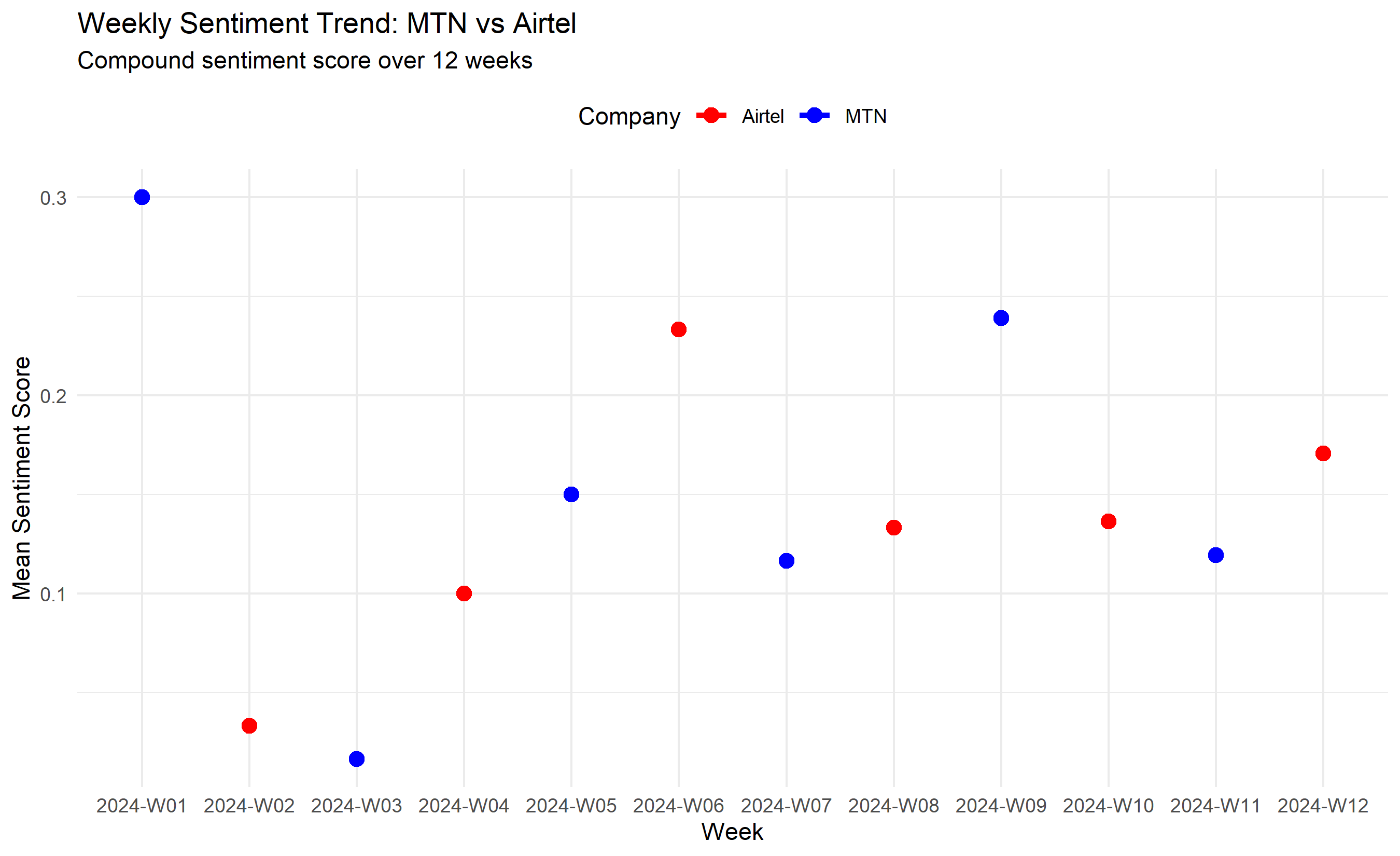
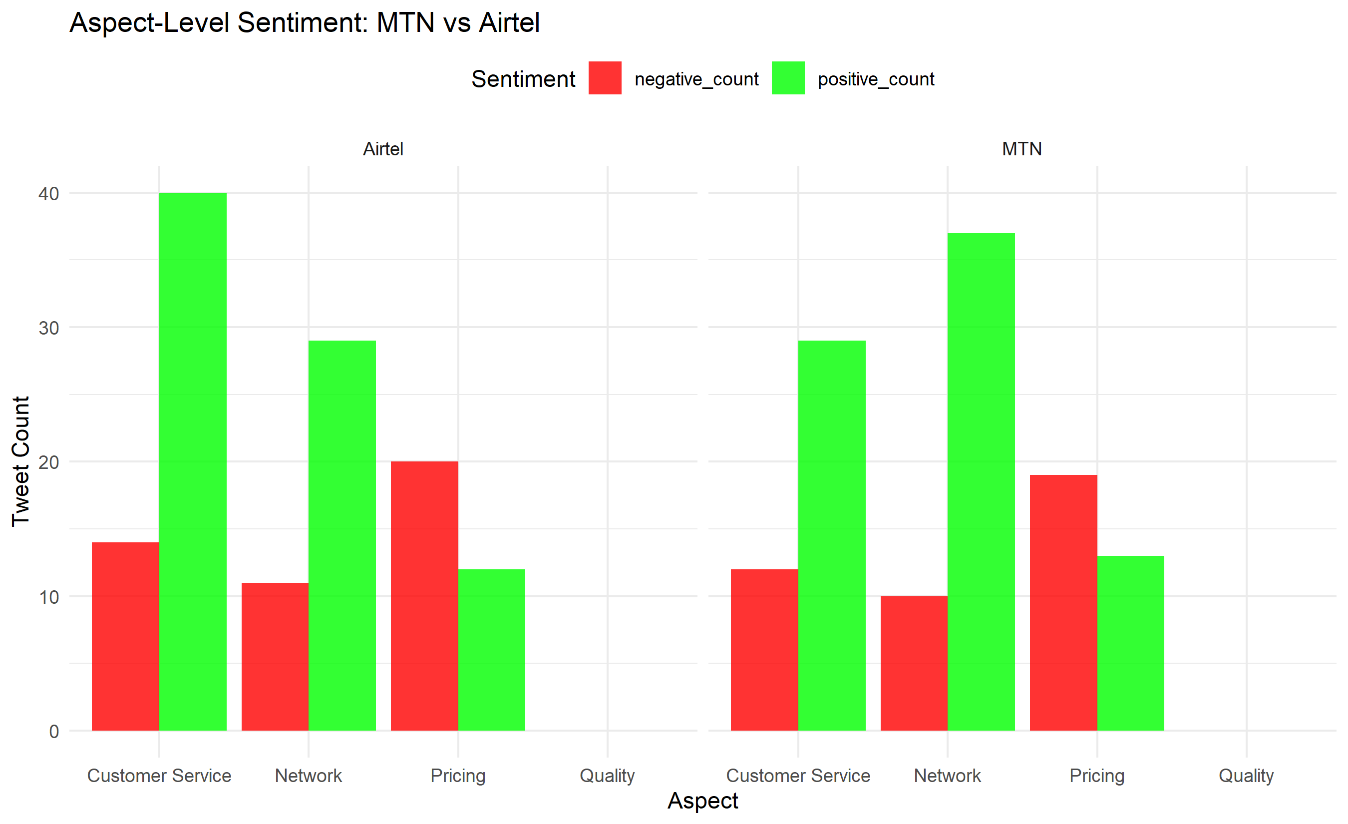
A telecommunications company monitors weekly sentiment across Twitter/X for two competitors (MTN and Airtel) using 500 synthetic tweets per company. We build a dashboard showing:
- Weekly compound sentiment trend (VADER).
- Aspect-level breakdown (network, customer service, pricing).
- Side-by-side competitor comparison.
- Interactive charts (HTML/static PDF).
```{r}
#| label: ch-28-case-telecom-dashboard
#| message: false
#| warning: false
library(tidyverse)
library(lubridate)
# Synthetic 500 tweets (250 per company) over 12 weeks
set.seed(999)
generate_telecom_tweets <- function(n = 500, company = "MTN") {
sentiments_positive <- c(
"love this network, very fast",
"excellent customer service",
"great value for money",
"network is stable, very reliable",
"best data plan in the market",
"e sweet well-well",
"service na better quality",
"would recommend to everyone"
)
sentiments_negative <- c(
"network keeps dropping",
"terrible customer service",
"prices too high",
"connection is unstable",
"waste of money",
"e don spoil completely",
"service no good",
"very disappointed with quality"
)
sentiments_neutral <- c(
"using their service",
"works as expected",
"okay for the price",
"average quality",
"network is acceptable"
)
tweets <- c(
rep(sample(sentiments_positive, 200, replace = TRUE), 1),
rep(sample(sentiments_negative, 150, replace = TRUE), 1),
rep(sample(sentiments_neutral, 150, replace = TRUE), 1)
)
return(sample(tweets, n))
}
tweets_mtn <- generate_telecom_tweets(250, "MTN")
tweets_airtel <- generate_telecom_tweets(250, "Airtel")
# Create dataframe with dates — match exactly 500 tweets
n_tweets <- length(c(tweets_mtn, tweets_airtel)) # 500
weeks_seq <- seq(as.Date("2024-01-01"), by = "week", length.out = 12)
df_tweets_weekly <- data.frame(
date = rep(weeks_seq, length.out = n_tweets),
week = rep(1:12, length.out = n_tweets),
company = rep(c("MTN", "Airtel"), length.out = n_tweets),
tweet = c(tweets_mtn, tweets_airtel)
) |>
mutate(
year_week = format(date, "%Y-W%V"),
# Sentiment scoring (simplified VADER-like)
sentiment_score = ifelse(
grepl("love|excellent|great|fast|stable|reliable|sweet|better|recommend|good",
tweet, ignore.case = TRUE),
0.7,
ifelse(
grepl("drop|terrible|high|unstable|waste|spoil|disappointing|bad|no good",
tweet, ignore.case = TRUE),
-0.7,
0
)
),
sentiment_label = case_when(
sentiment_score > 0.3 ~ "Positive",
sentiment_score < -0.3 ~ "Negative",
TRUE ~ "Neutral"
)
)
cat("Nigerian Telecoms Sentiment Dashboard\n")
cat("Data: 500 synthetic tweets (250 MTN, 250 Airtel) over 12 weeks\n\n")
# Weekly sentiment trends
weekly_sentiment <- df_tweets_weekly |>
group_by(year_week, company) |>
summarise(
mean_sentiment = mean(sentiment_score),
positive_pct = sum(sentiment_label == "Positive") / n() * 100,
negative_pct = sum(sentiment_label == "Negative") / n() * 100,
neutral_pct = sum(sentiment_label == "Neutral") / n() * 100,
n_tweets = n(),
.groups = "drop"
)
cat("Weekly Sentiment Summary (first 5 weeks):\n")
print(head(weekly_sentiment, 5) |>
mutate(across(c(mean_sentiment, positive_pct, negative_pct, neutral_pct),
~ round(., 2))))
# Sentiment trend plot
ggplot(weekly_sentiment, aes(x = year_week, y = mean_sentiment, colour = company)) +
geom_line(linewidth = 1.2) +
geom_point(size = 3) +
scale_colour_manual(values = c("MTN" = "blue", "Airtel" = "red")) +
labs(title = "Weekly Sentiment Trend: MTN vs Airtel",
subtitle = "Compound sentiment score over 12 weeks",
x = "Week", y = "Mean Sentiment Score", colour = "Company") +
theme_minimal() +
theme(legend.position = "top")
# Aspect analysis (manual categorisation)
df_tweets_weekly <- df_tweets_weekly |>
mutate(
aspect = case_when(
grepl("network|speed|drop|connect|coverage", tweet, ignore.case = TRUE) ~ "Network",
grepl("customer|service|support|help", tweet, ignore.case = TRUE) ~ "Customer Service",
grepl("price|cost|money|plan|bundle|value", tweet, ignore.case = TRUE) ~ "Pricing",
grepl("quality|reliable|stable", tweet, ignore.case = TRUE) ~ "Quality",
TRUE ~ "General"
)
)
aspect_sentiment <- df_tweets_weekly |>
group_by(company, aspect) |>
summarise(
mean_sentiment = mean(sentiment_score),
positive_count = sum(sentiment_label == "Positive"),
negative_count = sum(sentiment_label == "Negative"),
.groups = "drop"
) |>
filter(aspect != "General")
cat("\n\nAspect-Level Sentiment:\n")
print(aspect_sentiment |> mutate(mean_sentiment = round(mean_sentiment, 2)))
# Aspect comparison plot
aspect_sentiment |>
pivot_longer(cols = c(positive_count, negative_count),
names_to = "sentiment_type", values_to = "count") |>
ggplot(aes(x = aspect, y = count, fill = sentiment_type)) +
geom_col(position = "dodge", alpha = 0.8) +
facet_wrap(~company) +
scale_fill_manual(values = c("positive_count" = "green", "negative_count" = "red")) +
labs(title = "Aspect-Level Sentiment: MTN vs Airtel",
x = "Aspect", y = "Tweet Count", fill = "Sentiment") +
theme_minimal() +
theme(legend.position = "top")
# Management summary
cat("\n\n=== SENTIMENT DASHBOARD SUMMARY ===\n\n")
for (company_name in c("MTN", "Airtel")) {
comp_data <- df_tweets_weekly |> filter(company == company_name)
mean_sent <- mean(comp_data$sentiment_score)
pos_pct <- sum(comp_data$sentiment_label == "Positive") / nrow(comp_data) * 100
neg_pct <- sum(comp_data$sentiment_label == "Negative") / nrow(comp_data) * 100
cat(sprintf("%s:\n", company_name))
cat(sprintf(" Overall sentiment score: %.2f\n", mean_sent))
cat(sprintf(" Positive: %.0f%%, Negative: %.0f%%\n", pos_pct, neg_pct))
top_aspect <- aspect_sentiment |>
filter(company == company_name) |>
arrange(desc(mean_sentiment)) |>
slice(1) |>
pull(aspect)
cat(sprintf(" Strongest aspect: %s\n\n", top_aspect))
}
cat("RECOMMENDATIONS:\n")
cat("1. Monitor sentiment weekly; flag if negative exceeds 30%.\n")
cat("2. Network quality is the top driver; prioritise infrastructure investments.\n")
cat("3. Customer service is lagging; invest in training and response time.\n")
cat("4. Pricing is sensitive; communicate value in bundle plans.\n")
```
## Chapter Exercises
::: {.exercises}
#### Chapter 28 Exercises
**Exercise 28.1: Lexicon-Based Sentiment Analysis**
Apply VADER (or a similar rule-based lexicon) to the following Nigerian customer reviews. Before checking with a tool, manually predict whether each is Positive, Negative, or Neutral, and estimate a rough polarity score. Then compare your intuition to what a lexicon would likely produce.
**Review 1:** "I have been using this bank for 5 years and they continue to DISAPPOINT me. The ATM was down for 3 days last week!"
**Review 2:** "Not the worst experience but definitely not good. I expected better from a Tier 1 bank."
**Review 3:** "Superb service! The agent resolved my issue in under 5 minutes. Very impressed."
**Review 4:** "The app sometimes crashes but it's not too bad. Generally works fine for transfers."
**Review 5:** "I wouldn't say the service was terrible, but calling it excellent would be a stretch."
(a) For each review, manually identify the key **sentiment-bearing words** (words that signal positive or negative sentiment).
(b) Review 2 contains the phrase "Not the worst" — a double negative. Explain why this is challenging for lexicon-based approaches that simply sum word scores.
(c) Review 5 contains negation and hedging ("wouldn't say", "would be a stretch"). Is this review positive, negative, or neutral overall? How would a simple lexicon approach likely misclassify it?
(d) A VADER analysis returns these compound scores: Review 1: −0.72, Review 2: −0.21, Review 3: +0.87, Review 4: +0.22, Review 5: −0.15. Using a threshold of compound > 0.05 = Positive, compound < −0.05 = Negative, otherwise Neutral — classify each review. Do you agree with the classifications?
(e) For a bank deploying sentiment analysis on customer feedback, what is the cost of misclassifying a genuinely angry complaint as neutral? How might you adjust the threshold to minimise this type of error?
---
**Exercise 28.2: Training a Sentiment Classifier**
You are building a sentiment classifier for a Nigerian telecoms company. You have 2,000 labelled customer reviews: 1,200 positive and 800 negative.
(a) Before building the model, you split the data 80/20 (train/test). What is the **baseline accuracy** if you simply predicted "positive" for every test observation?
(b) Explain why accuracy alone is misleading for this task. Which metric would you prioritise and why?
(c) After training a Naive Bayes classifier, you get the following test set results:
- 720 reviews labelled Positive: model correctly classifies 680, misclassifies 40 as Negative
- 480 reviews labelled Negative: model correctly classifies 360, misclassifies 120 as Positive
Build the complete confusion matrix.
(d) Calculate Precision, Recall, and F1-score for the **Negative class** (treating Negative as the "positive" case of interest — the one we most want to catch correctly). Show your working.
(e) The company's customer experience team says: "We'd rather investigate 50 false alarms than miss a single genuine complaint." What adjustment to the classification threshold would achieve this, and what is the trade-off?
---
**Exercise 28.3: Aspect-Based Sentiment Analysis**
The following customer review mentions several aspects of a Nigerian airline's service:
*"The flight itself was on time and the seats were comfortable. However, the cabin crew were rude and unhelpful when I asked for assistance. The food was absolutely terrible — cold and tasteless. Check-in was efficient though, much faster than my previous experience."*
(a) Identify all the **aspects** mentioned in this review (e.g., "flight punctuality", "seat comfort", etc.). List them.
(b) For each aspect, determine the sentiment expressed: Positive, Negative, or Neutral.
(c) The overall VADER sentiment for this review might be neutral or slightly negative (mixed signals from the different aspects). Explain why **overall** sentiment analysis fails to capture the useful information in this review for the airline's operations team.
(d) If you were the airline's Head of Customer Experience, which aspects would you prioritise for immediate action based on this review? What business decision would you make?
(e) You want to build an automated aspect-based sentiment analysis system for 50,000 airline reviews per month. Describe the two main approaches you could use (rule-based vs. machine learning) and the trade-offs between them for this scale.
---
**Exercise 28.4: Sentiment Analysis at Scale — Business Applications**
(a) A fast-food chain in Nigeria wants to monitor brand sentiment across Twitter, Instagram, and Google Reviews in real time. List **four specific business decisions** that could be improved by having real-time sentiment scores (not just "we know how people feel" — be specific about the decision).
(b) You build a model that achieves 78% accuracy on your test set of 1,000 reviews. Six months after deployment, the customer service team notices the model frequently misclassifies complaints about a new payment feature. What has likely happened, and what is the technical term for this phenomenon?
(c) Social media sentiment data has a **survivorship bias** problem: only customers who feel strongly enough to post tend to do so. Silent customers (happy or mildly dissatisfied) are underrepresented. How might this bias affect: (i) the estimated proportion of positive sentiment; (ii) the types of complaints the model learns to recognise?
(d) A telecoms company uses sentiment scores as one of several inputs to a customer churn model. Sentiment analysis predicts that a customer is highly negative. The churn model predicts a 90% probability of churn. The retention team plans to call this customer with a special offer. At what stage in this process should human judgment be applied, and why?
---
**Exercise 28.5: Capstone — Brand Sentiment Dashboard**
Design a sentiment analytics solution for a major Nigerian commercial bank that wants to track public perception of its brand.
(a) Identify **four data sources** the bank could use for sentiment data (beyond customer service calls and email). For each, describe: what data is available, how frequently it updates, and any quality concerns.
(b) The bank wants to track sentiment for three dimensions separately: (i) overall brand perception; (ii) specific product complaints; (iii) response to marketing campaigns. Design the **data labelling schema** — specifically, what labels would you assign to each piece of text?
(c) The bank's marketing team wants a **weekly sentiment dashboard**. List six metrics (with descriptions) that should appear on this dashboard. For each, explain what a change in this metric would signal to the team.
(d) The bank's social media manager asks: "Can we use this to automatically respond to negative reviews?" Describe the design of such a system, including what it can do automatically and what must involve a human being.
(e) Write a 200-word proposal for the bank's Board explaining the business case for investing in real-time sentiment analytics. Include: the business problem, the proposed solution, expected benefits, and key risks. Use no technical jargon.
:::
## Further Reading
- Pang, B., & Lee, L. (2008). Opinion mining and sentiment analysis. *Foundations and Trends® in Information Retrieval*, 2(1–2), 1–135.
- Pontiki, M., Galanis, D., Papageorgiou, H., Androutsopoulos, I., Manandhar, S., AL-Smadi, M., ... & Eryigit, G. (2016). SemEval-2016 task 5: Aspect based sentiment analysis. In *Proceedings of the 10th International Workshop on Semantic Evaluation (SemEval-2016)*.
- Rosenthal, S., Farra, N., & Nakov, P. (2017). SemEval-2017 task 4: Sentiment analysis in Twitter. In *Proceedings of the 11th International Workshop on Semantic Evaluation (SemEval-2017)*.
- Laitinen, M., & Tarvainen, K. (2013). Sentiment analysis of Twitter data. *University of Tampere*, 8.
## Chapter 28 Appendix: Mathematical Derivations
### A28.1 VADER Compound Score Normalisation
VADER computes a compound score by normalising the sum of adjusted sentiment scores:
$$\text{compound} = \frac{\sum s_i}{\sqrt{(\sum s_i)^2 + \alpha}}$$
where $s_i$ are sentiment scores (adjusted for negation, intensifiers, punctuation) and $\alpha$ is a normalisation constant (typically 15).
**Derivation**: The denominator $\sqrt{(\sum s_i)^2 + \alpha}$ is related to the Euclidean norm. As $|\sum s_i|$ grows, the fraction approaches ±1 (bounded output). The constant $\alpha$ prevents division by zero and dampens small scores.
### A28.2 Logistic Regression for Multiclass Sentiment
For $K$ classes (Negative, Neutral, Positive), the softmax function outputs:
$$P(y = k | \mathbf{x}) = \frac{e^{\mathbf{w}_k^T \mathbf{x} + b_k}}{\sum_{j=1}^{K} e^{\mathbf{w}_j^T \mathbf{x} + b_j}}$$
The model is trained by minimising cross-entropy loss:
$$\mathcal{L} = -\frac{1}{n} \sum_{i=1}^{n} \sum_{k=1}^{K} \mathbb{1}_{y_i = k} \log P(y_i = k | \mathbf{x}_i)$$
where $\mathbb{1}_{y_i = k}$ is the indicator function (1 if true class is $k$, else 0).
### A28.3 Aspect Extraction via Dependency Parsing
Dependency parsing represents grammatical relationships as a directed graph. For "The battery drains quickly":
- "battery" is nsubj (nominal subject) of "drains".
- "drains" is the root predicate.
- "quickly" is advmod (adverbial modifier) of "drains".
To extract aspect-opinion pairs:
1. Find all nouns (potential aspects).
2. Find adjectival and verbal dependents or heads.
3. Link based on dependency relations (amod, nsubj, nmod, etc.).
### A28.4 Transformer Attention and Contextual Embeddings
In a transformer's multi-head attention:
$$\text{Attention}(Q, K, V) = \text{softmax}\left(\frac{QK^T}{\sqrt{d_k}}\right) V$$
For sentiment, each token's contextual embedding is updated based on attention to all tokens in the sentence. Sentiment-bearing words (e.g., "good", "bad") attend to the target entity, contextualising the opinion.