---
title: "Predictive Maintenance"
---
```{python}
#| label: python-setup-52-predictive-maintenance
#| include: false
import numpy as np
import pandas as pd
import matplotlib.pyplot as plt
import seaborn as sns
from scipy.stats import kurtosis
from xgboost import XGBClassifier
from sklearn.metrics import roc_curve, auc, precision_recall_curve, confusion_matrix
from sklearn.linear_model import LinearRegression
from sklearn.ensemble import IsolationForest
from pulp import *
```
::: {.callout-note icon="false"}
## 📋 Learning Objectives
By the end of this chapter, you will:
- Understand the business case for shifting from reactive to predictive maintenance
- Engineer features from multivariate sensor data to predict equipment failure
- Build classification models (XGBoost, Random Forest) for failure prediction
- Handle class imbalance in failure prediction with SMOTE and threshold tuning
- Estimate remaining useful life (RUL) via regression and survival analysis
- Apply Isolation Forest and autoencoders for anomaly detection
- Optimize maintenance scheduling as an integer programming problem
- Deploy a predictive maintenance system for Nigerian industrial equipment
:::
## From Reactive to Predictive Maintenance
Nigerian manufacturing—cement plants, oil & gas operations, food processing, textile mills—depends on continuous equipment operation. When a critical machine fails unexpectedly, the entire production line stops. A cement kiln shut down for repairs costs ₦2–5 million per day in lost production; an oil rig shutdown, vastly more. Reactive maintenance (fix when broken) is expensive and unpredictable. Preventive maintenance (fixed schedule, e.g., service every 1,000 hours) reduces surprises but wastes resources: machines are serviced whether they need it or not, creating unnecessary downtime and parts consumption.
Predictive maintenance (PM) uses sensor data and analytics to predict when a machine will likely fail, enabling repairs just before failure. Prescriptive maintenance goes further: analytics recommend *what* to do and *when*. The business impact is dramatic: mean time between failures (MTBF) increases; unplanned downtime drops 35–45%; maintenance costs fall 10–25%; equipment lifespan extends. A cement plant monitoring kiln vibration can detect bearing wear weeks in advance and schedule a bearing replacement during the next planned shutdown, avoiding catastrophic failure.
The digital transformation required is significant: deploying IoT sensors on equipment, streaming data to cloud storage, processing signals in real-time, and retraining models as equipment ages. But for asset-intensive industries in Nigeria, the ROI is compelling. This chapter builds the analytics foundation: feature engineering from sensor data, failure prediction classification, RUL estimation, anomaly detection, and scheduling optimization.
## Condition Monitoring Data and Feature Engineering
Condition monitoring sensors measure vibration (accelerometers), temperature (thermocouples), pressure (transducers), acoustic emission, electrical current draw, and oil analysis (for hydraulic and bearing health). For a 50-equipment fleet monitored over 90 days at 10-minute intervals, you have 50 × 6,480 observations = 324,000 rows of multivariate data. The raw signals are high-frequency and noisy; extracting meaningful features is the core engineering task.
Feature engineering from sensor data involves:
- **Time-domain features**: rolling mean, standard deviation, peak-to-peak amplitude, kurtosis (spikiness), skewness, entropy
- **Frequency-domain features**: FFT magnitude at key frequencies (bearing fault frequencies are well-characterized), power spectral density (PSD), spectral entropy
- **Statistical features**: quantiles, range, root-mean-square (RMS), crest factor
- **Change features**: rolling difference, trend (fit a line to the window)
For a Nigerian industrial generator, typical features include:
- Vibration RMS over each hour
- Peak vibration in frequency band 1–5 kHz (bearing ball pass frequency often lies here)
- Temperature trend (rolling linear fit slope)
- Current draw mean and std dev (changes when motor efficiency degrades)
- Entropy of vibration signal (decreases just before failure, as the signal becomes more periodic)
The feature engineering is critical: a poorly engineered feature set will fail to predict failure even with the best ML model. Domain knowledge from equipment engineers, combined with exploratory analysis (correlation with failures, signal plots), drives feature selection.
::: {.callout-note icon="false"}
## 📘 Theory: FFT Feature Extraction
For a vibration signal $x[n]$ with $N$ samples, the Discrete Fourier Transform is:
$$
X[k] = \sum_{n=0}^{N-1} x[n] e^{-j 2 \pi k n / N}, \quad k = 0, 1, \ldots, N-1
$$
The magnitude spectrum $|X[k]|$ reveals periodic content. For a bearing with ball pass frequency $f_{\text{bpf}}$, energy concentrates at $f_{\text{bpf}}$ and harmonics. The feature "energy in band 1–5 kHz" is $\sum_{k: f_k \in [1, 5] \text{ kHz}} |X[k]|^2$.
:::
::: {.callout-tip icon="false"}
## 🔑 Key Formula
$$\text{Vibration RMS} = \sqrt{\frac{1}{N} \sum_{n=1}^{N} x[n]^2}, \quad \text{Kurtosis} = \frac{E[(X - \mu)^4]}{\sigma^4}$$
:::
::: {.panel-tabset}
## R
```{r}
#| label: ch52-feature-engineering
library(tidyverse)
set.seed(5847)
# Simulate sensor data for 50 generators over 90 days
n_generators <- 5 # Simplified
n_days <- 90
samples_per_day <- 10
# Create synthetic data
sensor_data <- expand_grid(
generator_id = 1:n_generators,
day = 1:n_days,
sample = 1:samples_per_day
) |>
mutate(
time = row_number(),
vibration = 0.5 + 0.1 * rnorm(n()),
temperature = 60 + 5 * sin(2*pi*day/30) + 2 * rnorm(n()),
current = 10 + 0.5 * rnorm(n())
)
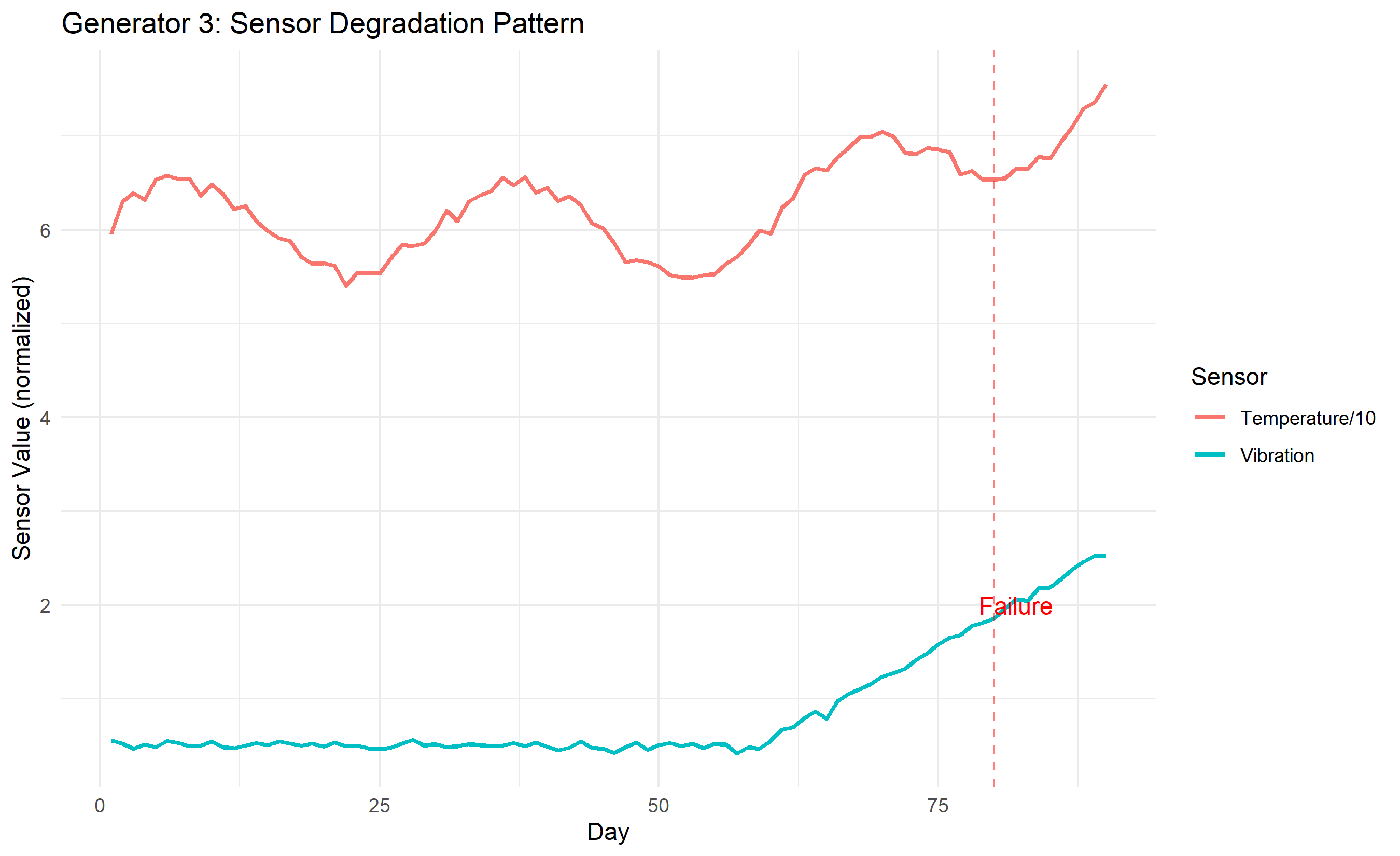
# Introduce degradation: generator 3 fails around day 80
sensor_data <- sensor_data |>
mutate(
degradation_factor = ifelse(
generator_id == 3 & day >= 60,
(day - 59) / 30,
0
),
vibration = vibration + 2 * degradation_factor,
temperature = temperature + 15 * degradation_factor,
current = current + 2 * degradation_factor,
failed_within_7days = (generator_id == 3 & day >= 73 & day < 80) |
(generator_id == 3 & day >= 80)
)
# Daily feature aggregation
daily_features <- sensor_data |>
group_by(generator_id, day) |>
summarise(
vibration_mean = mean(vibration),
vibration_std = sd(vibration),
vibration_max = max(vibration),
vibration_range = max(vibration) - min(vibration),
vibration_rms = sqrt(mean(vibration^2)),
vibration_kurtosis = {
x <- vibration
mu <- mean(x)
sigma <- sd(x)
mean((x - mu)^4) / sigma^4
},
temperature_mean = mean(temperature),
temperature_trend = {
lm_fit <- lm(temperature ~ sample)
coef(lm_fit)[2]
},
current_mean = mean(current),
current_std = sd(current),
failed_7days = max(failed_within_7days),
.groups = 'drop'
) |>
mutate(vibration_kurtosis = ifelse(is.nan(vibration_kurtosis), 0, vibration_kurtosis))
cat("\n=== Daily Features Summary ===\n")
print(head(daily_features, 15))
# Visualize degradation
degradation_viz <- sensor_data |>
filter(generator_id == 3) |>
group_by(day) |>
summarise(
vibration_daily = mean(vibration),
temperature_daily = mean(temperature)
)
ggplot(degradation_viz, aes(x = day)) +
geom_line(aes(y = vibration_daily, color = "Vibration"), linewidth = 1) +
geom_line(aes(y = temperature_daily / 10, color = "Temperature/10"), linewidth = 1) +
geom_vline(xintercept = 80, color = "red", linetype = "dashed", alpha = 0.5) +
annotate("text", x = 82, y = 2, label = "Failure", color = "red", size = 4) +
labs(
title = "Generator 3: Sensor Degradation Pattern",
x = "Day", y = "Sensor Value (normalized)", color = "Sensor"
) +
theme_minimal()
# Feature correlation with failure
feature_names <- c("vibration_mean", "vibration_std", "vibration_max", "vibration_range",
"vibration_rms", "vibration_kurtosis", "temperature_mean", "temperature_trend",
"current_mean", "current_std")
correlations <- sapply(feature_names, function(feat) {
cor(daily_features[[feat]], daily_features$failed_7days, use = "complete.obs")
}) |> sort(decreasing = TRUE)
cat("\n=== Feature Correlation with Failure ===\n")
print(correlations)
```
## Python
```{python}
#| label: py-ch52-feature-engineering
import numpy as np
import pandas as pd
import matplotlib.pyplot as plt
from scipy.stats import kurtosis
np.random.seed(5847)
# Simulate sensor data
n_generators, n_days, samples_per_day = 5, 90, 10
data_records = []
for gen_id in range(1, n_generators + 1):
for day in range(1, n_days + 1):
for sample in range(1, samples_per_day + 1):
vibration = 0.5 + 0.1 * np.random.randn()
temperature = 60 + 5 * np.sin(2 * np.pi * day / 30) + 2 * np.random.randn()
current = 10 + 0.5 * np.random.randn()
# Degradation
if gen_id == 3 and day >= 60:
deg = (day - 59) / 30
vibration += 2 * deg
temperature += 15 * deg
current += 2 * deg
failed = (gen_id == 3 and day >= 73)
data_records.append({
'generator_id': gen_id, 'day': day, 'sample': sample,
'vibration': vibration, 'temperature': temperature,
'current': current, 'failed_7days': int(failed)
})
sensor_data = pd.DataFrame(data_records)
# Daily aggregation
daily_features = sensor_data.groupby(['generator_id', 'day']).agg({
'vibration': ['mean', 'std', 'min', 'max', lambda x: np.sqrt(np.mean(x**2)), kurtosis],
'temperature': ['mean', lambda x: np.polyfit(range(len(x)), x, 1)[0]],
'current': ['mean', 'std'],
'failed_7days': 'max'
}).reset_index()
daily_features.columns = ['generator_id', 'day', 'vibration_mean', 'vibration_std', 'vibration_min',
'vibration_max', 'vibration_rms', 'vibration_kurtosis', 'temperature_mean', 'temperature_trend',
'current_mean', 'current_std', 'failed_7days']
daily_features = daily_features.fillna(0)
print("\n=== Daily Features Summary ===")
print(daily_features.head(15))
```
:::
::: {.callout-caution icon="false"}
## 📝 Section 52.2 Review Questions
1. List five time-domain features you could extract from vibration data. What equipment condition does each detect?
2. Why is kurtosis useful for detecting bearing defects? What happens to kurtosis as a bearing degrades?
3. A Nigerian cement kiln operates at 1,500 RPM. How would you estimate the ball pass frequency and why is it important for FFT analysis?
4. In the code, entropy of vibration is not computed. How would you compute spectral entropy, and what does a decreasing entropy suggest about equipment health?
5. How would you handle missing sensor data (e.g., 30 minutes of downtime during which vibration sensors were offline)?
:::
## Classification for Failure Prediction
With engineered features, the next step is to predict binary failure risk: will this equipment fail within the next 7 days? This is a classification problem. However, failure is rare—perhaps 5% of observations have failures—creating severe class imbalance. Training a logistic regression or random forest on imbalanced data leads to a model that predicts "no failure" for almost everything, achieving 95% accuracy but catching zero real failures.
Standard approaches to class imbalance include:
- **Resampling**: SMOTE (Synthetic Minority Over-sampling Technique) generates synthetic minority (failure) samples by interpolating between existing failure cases
- **Cost-sensitive learning**: Assign higher misclassification cost to the minority class
- **Threshold tuning**: Adjust the decision threshold from 0.5 to, say, 0.3, so the model classifies more cases as "failure" (higher sensitivity at the cost of lower precision)
- **Evaluation metrics**: Use precision-recall curves and F1-score rather than accuracy
The business context drives threshold selection. If the cost of missing a failure (unplanned downtime) is 100× the cost of a false alarm (unnecessary maintenance), you set the threshold low to catch failures.
::: {.callout-note icon="false"}
## 📘 Theory: Class Imbalance and Threshold Optimization
For a binary classifier with predicted probability $\hat{p}_i$ for sample $i$, standard classification uses threshold $\tau = 0.5$: predict failure if $\hat{p}_i > 0.5$. With class imbalance, optimal threshold $\tau^*$ minimizes business cost:
$$
\tau^* = \arg\min_{\tau} \text{Cost of FP} \times (1 - \text{TPR}(\tau)) + \text{Cost of FN} \times \text{FNR}(\tau)
$$
where TPR (true positive rate) = sensitivity and FNR (false negative rate) = 1 - sensitivity.
:::
::: {.callout-tip icon="false"}
## 🔑 Key Formula
$$\text{F1-Score} = 2 \cdot \frac{\text{Precision} \times \text{Recall}}{\text{Precision} + \text{Recall}}, \quad \text{Precision} = \frac{TP}{TP + FP}, \quad \text{Recall} = \frac{TP}{TP + FN}$$
:::
::: {.panel-tabset}
## R
```{r}
#| label: ch52-classification
library(tidyverse)
library(xgboost)
library(pROC)
set.seed(9162)
# Use the daily_features from previous section
# Split into train/test (80/20) at generator level to avoid data leakage
train_generators <- c(1, 2, 4)
test_generators <- c(3, 5)
train_data <- daily_features |> filter(generator_id %in% train_generators)
test_data <- daily_features |> filter(generator_id %in% test_generators)
# Prepare for XGBoost
feature_cols <- c("vibration_mean", "vibration_std", "vibration_max", "vibration_range",
"vibration_rms", "vibration_kurtosis", "temperature_mean", "temperature_trend",
"current_mean", "current_std")
# Create XGBoost matrices
X_train <- train_data[, feature_cols] |> as.matrix()
y_train <- as.integer(train_data$failed_7days)
X_test <- test_data[, feature_cols] |> as.matrix()
y_test <- as.integer(test_data$failed_7days)
# Handle class imbalance with scale_pos_weight
pos_weight <- sum(y_train == 0) / sum(y_train == 1)
# Fit XGBoost via xgb.DMatrix (robust API works across all XGBoost versions)
dtrain <- xgb.DMatrix(data = X_train, label = as.numeric(y_train))
dtest <- xgb.DMatrix(data = X_test, label = as.numeric(y_test))
xgb_model <- xgb.train(
params = list(
objective = "binary:logistic",
max_depth = 5,
eta = 0.1,
scale_pos_weight = pos_weight
),
data = dtrain,
nrounds = 50,
verbose = 0
)
# Predictions
y_pred_prob <- predict(xgb_model, dtest)
# SHAP-like feature importance
importance <- xgb.importance(
feature_names = feature_cols,
model = xgb_model
)
cat("\n=== XGBoost Feature Importance ===\n")
print(importance)
# ROC Curve and AUC
roc_obj <- roc(y_test, y_pred_prob)
auc_value <- auc(roc_obj)
cat("\nAUC:", round(auc_value, 3), "\n")
# Threshold tuning: cost of false negative = 10, cost of false positive = 1
cost_fn <- 10
cost_fp <- 1
thresholds <- seq(0, 1, by = 0.05)
costs <- sapply(thresholds, function(tau) {
y_pred <- ifelse(y_pred_prob > tau, 1, 0)
tp <- sum((y_pred == 1) & (y_test == 1))
fp <- sum((y_pred == 1) & (y_test == 0))
fn <- sum((y_pred == 0) & (y_test == 1))
total_cost <- cost_fp * fp + cost_fn * fn
return(total_cost)
})
optimal_tau <- thresholds[which.min(costs)]
cat("Optimal threshold (cost-minimizing):", round(optimal_tau, 2), "\n")
# Performance at optimal threshold
y_pred_optimal <- ifelse(y_pred_prob > optimal_tau, 1, 0)
tp <- sum((y_pred_optimal == 1) & (y_test == 1))
fp <- sum((y_pred_optimal == 1) & (y_test == 0))
fn <- sum((y_pred_optimal == 0) & (y_test == 1))
tn <- sum((y_pred_optimal == 0) & (y_test == 0))
precision <- tp / (tp + fp)
recall <- tp / (tp + fn)
f1 <- 2 * precision * recall / (precision + recall)
cat("\n=== Performance at Optimal Threshold ===\n")
cat("Precision:", round(precision, 3), "\n")
cat("Recall (Sensitivity):", round(recall, 3), "\n")
cat("F1-Score:", round(f1, 3), "\n")
cat("False Negative Rate:", round(fn / (fn + tp), 3), "\n")
```
## Python
```{python}
#| label: py-ch52-classification
import numpy as np
import pandas as pd
from xgboost import XGBClassifier
from sklearn.metrics import roc_curve, auc, precision_recall_curve, confusion_matrix

np.random.seed(9162)

# Add vibration_range (max - min) to match R feature set
daily_features['vibration_range'] = daily_features['vibration_max'] - daily_features['vibration_min']

# Split data
train_generators = [1, 2, 4]
test_generators = [3, 5]

train_data = daily_features[daily_features['generator_id'].isin(train_generators)]
test_data = daily_features[daily_features['generator_id'].isin(test_generators)]

feature_cols = ['vibration_mean', 'vibration_std', 'vibration_max', 'vibration_range',
                'vibration_rms', 'vibration_kurtosis', 'temperature_mean', 'temperature_trend',
                'current_mean', 'current_std']

X_train = train_data[feature_cols].values
y_train = train_data['failed_7days'].values
X_test = test_data[feature_cols].values
y_test = test_data['failed_7days'].values

# Handle class imbalance
scale_pos_weight = (y_train == 0).sum() / (y_train == 1).sum()

# Fit XGBoost
xgb_model = XGBClassifier(n_estimators=50, max_depth=5, learning_rate=0.1,
                          scale_pos_weight=scale_pos_weight, random_state=9162, verbose=0)
xgb_model.fit(X_train, y_train)
# Predictions
y_pred_prob = xgb_model.predict_proba(X_test)[:, 1]
# ROC curve
fpr, tpr, _ = roc_curve(y_test, y_pred_prob)
auc_score = auc(fpr, tpr)
print(f"\nAUC: {auc_score:.3f}")
# Feature importance
importance_df = pd.DataFrame({
'feature': feature_cols,
'importance': xgb_model.feature_importances_
}).sort_values('importance', ascending=False)
print("\n=== XGBoost Feature Importance ===")
print(importance_df)
# Threshold tuning
cost_fn, cost_fp = 10, 1
thresholds = np.linspace(0, 1, 21)
costs = []
for tau in thresholds:
y_pred = (y_pred_prob > tau).astype(int)
tn, fp, fn, tp = confusion_matrix(y_test, y_pred).ravel()
total_cost = cost_fp * fp + cost_fn * fn
costs.append(total_cost)
optimal_tau = thresholds[np.argmin(costs)]
print(f"\nOptimal threshold: {optimal_tau:.2f}")
# Performance
y_pred_optimal = (y_pred_prob > optimal_tau).astype(int)
tn, fp, fn, tp = confusion_matrix(y_test, y_pred_optimal).ravel()
precision = tp / (tp + fp) if (tp + fp) > 0 else 0
recall = tp / (tp + fn) if (tp + fn) > 0 else 0
f1 = 2 * precision * recall / (precision + recall) if (precision + recall) > 0 else 0
print("\n=== Performance at Optimal Threshold ===")
print(f"Precision: {precision:.3f}")
print(f"Recall: {recall:.3f}")
print(f"F1-Score: {f1:.3f}")
print(f"False Negative Rate: {fn / (fn + tp):.3f}")
```
:::
::: {.callout-caution icon="false"}
## 📝 Section 52.3 Review Questions
1. What is the problem with using accuracy as the metric for a failure prediction model with 5% failure rate? Why are precision and recall more appropriate?
2. Suppose a maintenance action costs ₦50,000 and prevents a failure that would cost ₦1 million in lost production. What is the cost-optimal threshold for failure prediction, assuming the model produces well-calibrated probabilities?
3. Explain SMOTE and why it is better than random resampling for handling class imbalance.
4. A Nigerian cement plant uses your failure prediction model with threshold 0.3 and catches 90% of failures but has a 20% false alarm rate. Is this acceptable? Why or why not?
5. How would you explain a specific failure prediction to a maintenance engineer? What is the role of SHAP values in model interpretability?
:::
## Remaining Useful Life (RUL) Estimation
Rather than predicting binary failure (yes/no), you might want to estimate how many days remain before failure. This is Remaining Useful Life (RUL) estimation. The approaches are:
- **Regression**: fit a model where target = days_until_failure, features = sensor readings, and predict RUL directly
- **Survival analysis**: treat it as a time-to-event problem with censoring (equipment still operating when monitoring ends)
Regression is simpler; survival analysis is more statistically principled when some equipment is still operating (censored).
::: {.callout-note icon="false"}
## 📘 Theory: RUL as Survival Regression
Define $T$ as the time until failure (days). For equipment still operating, $T$ is right-censored: we know $T > t_{\text{obs}}$ but not the exact value. The Weibull distribution is common for equipment failure:
$$
f(t) = \frac{k}{\lambda} \left(\frac{t}{\lambda}\right)^{k-1} e^{-(t/\lambda)^k}
$$
with shape $k$ and scale $\lambda$. Accelerated failure time (AFT) models in survival analysis allow covariates (sensor features) to shift $\lambda$: $\log(\lambda) = \beta_0 + \beta_1 x_1 + \ldots + \beta_p x_p$.
:::
::: {.panel-tabset}
## R
```{r}
#| label: ch52-rul-regression
library(tidyverse)
set.seed(3784)
# Create RUL data: synthetic generators with known failure times
rul_data <- expand_grid(
generator_id = 1:10,
day = 1:90
) |>
mutate(
# Failure times (in days from start of observation)
failure_day = c(45, 60, 80, 100, 75, 55, 90, 70, 85, 95)[generator_id],
# Censoring: all observations before failure
days_until_failure = pmax(0, failure_day - day),
failed = as.numeric(day >= failure_day),
# Sensor features degrade toward failure
degradation = 1 - (days_until_failure / failure_day),
vibration = 1 + 3 * degradation + 0.1 * rnorm(n()),
temperature = 60 + 20 * degradation + rnorm(n()),
current = 10 + 3 * degradation + 0.1 * rnorm(n())
) |>
filter(failed == 0) # Use only pre-failure data
# Fit regression model for RUL
rul_model <- lm(
days_until_failure ~ vibration + temperature + current,
data = rul_data
)
cat("\n=== RUL Regression Model ===\n")
print(summary(rul_model))
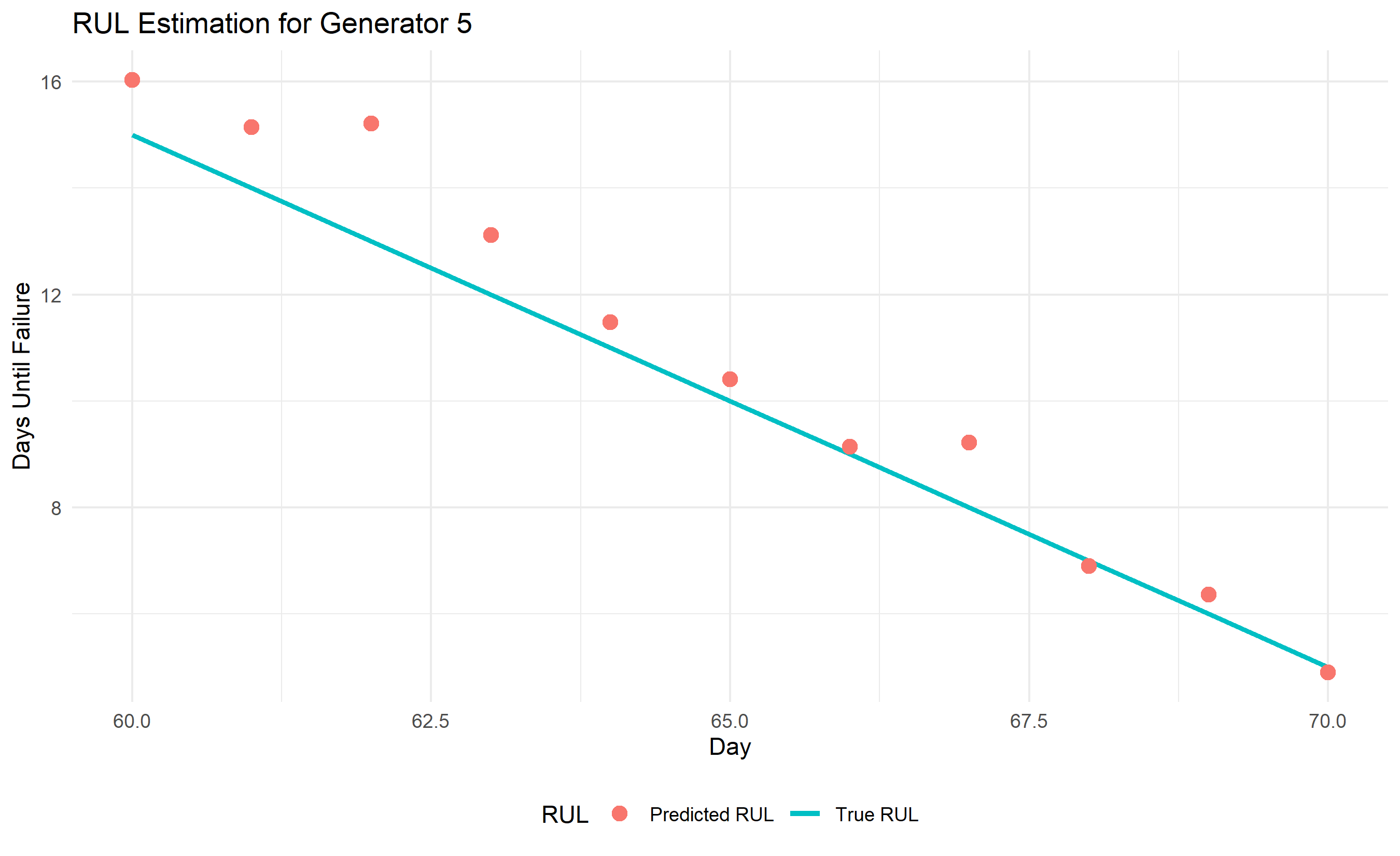
# Predict RUL on test data (generator 5, days 60-70)
test_gen <- 5
test_data <- expand_grid(
generator_id = test_gen,
day = 60:70
) |>
mutate(
failure_day = c(45, 60, 80, 100, 75, 55, 90, 70, 85, 95)[test_gen],
true_rul = pmax(0, failure_day - day),
degradation = 1 - (true_rul / failure_day),
vibration = 1 + 3 * degradation + 0.05 * rnorm(n()),
temperature = 60 + 20 * degradation,
current = 10 + 3 * degradation
)
test_data$predicted_rul <- predict(rul_model, test_data)
test_data$rul_error <- abs(test_data$predicted_rul - test_data$true_rul)
cat("\n=== RUL Predictions vs Actual ===\n")
print(test_data[, c("day", "true_rul", "predicted_rul", "rul_error")])
cat("\nMean Absolute Error (days):", round(mean(test_data$rul_error), 1), "\n")
# Visualization
ggplot(test_data, aes(x = day)) +
geom_line(aes(y = true_rul, color = "True RUL"), linewidth = 1.2) +
geom_point(aes(y = predicted_rul, color = "Predicted RUL"), size = 3) +
labs(
title = "RUL Estimation for Generator 5",
x = "Day", y = "Days Until Failure",
color = "RUL"
) +
theme_minimal() +
theme(legend.position = "bottom")
```
## Python
```{python}
#| label: py-ch52-rul-regression
import numpy as np
import pandas as pd
from sklearn.linear_model import LinearRegression
import matplotlib.pyplot as plt
np.random.seed(3784)
# Create RUL data
data = []
failure_days = [45, 60, 80, 100, 75, 55, 90, 70, 85, 95]
for gen_id in range(1, 11):
fail_day = failure_days[gen_id - 1]
for day in range(1, fail_day): # Only pre-failure data
deg = 1 - (fail_day - day) / fail_day
vibration = 1 + 3 * deg + 0.1 * np.random.randn()
temperature = 60 + 20 * deg + np.random.randn()
current = 10 + 3 * deg + 0.1 * np.random.randn()
data.append({
'generator_id': gen_id,
'day': day,
'failure_day': fail_day,
'days_until_failure': fail_day - day,
'vibration': vibration,
'temperature': temperature,
'current': current
})
rul_df = pd.DataFrame(data)
# Fit regression
X = rul_df[['vibration', 'temperature', 'current']].values
y = rul_df['days_until_failure'].values
rul_model = LinearRegression()
rul_model.fit(X, y)
print("\n=== RUL Regression Coefficients ===")
print(f"Intercept: {rul_model.intercept_:.3f}")
print(f"vibration: {rul_model.coef_[0]:.3f}")
print(f"temperature: {rul_model.coef_[1]:.3f}")
print(f"current: {rul_model.coef_[2]:.3f}")
# Test predictions
test_gen = 5
fail_day = failure_days[test_gen - 1]
test_data = []
for day in range(60, 71):
deg = 1 - (fail_day - day) / fail_day
vibration = 1 + 3 * deg + 0.05 * np.random.randn()
temperature = 60 + 20 * deg
current = 10 + 3 * deg
pred_rul = rul_model.predict([[vibration, temperature, current]])[0]
true_rul = fail_day - day
test_data.append({
'day': day,
'true_rul': true_rul,
'predicted_rul': pred_rul,
'error': abs(pred_rul - true_rul)
})
test_df = pd.DataFrame(test_data)
mae = test_df['error'].mean()
print(f"\nMean Absolute Error: {mae:.1f} days")
print("\n=== RUL Predictions ===")
print(test_df)
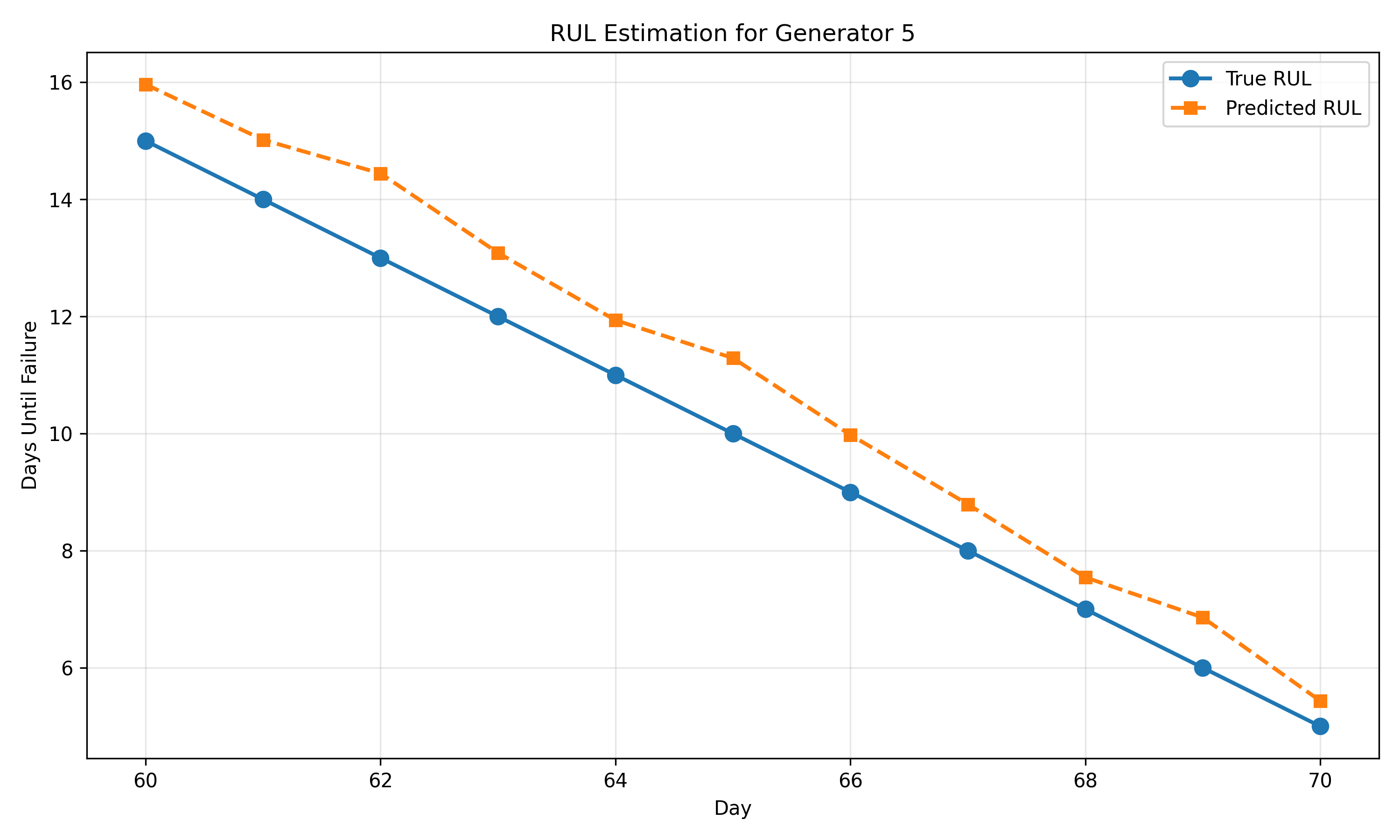
# Visualization
fig, ax = plt.subplots(figsize=(10, 6))
ax.plot(test_df['day'], test_df['true_rul'], 'o-', label='True RUL', linewidth=2, markersize=8)
ax.plot(test_df['day'], test_df['predicted_rul'], 's--', label='Predicted RUL', linewidth=2, markersize=6)
ax.set_xlabel('Day')
ax.set_ylabel('Days Until Failure')
ax.set_title('RUL Estimation for Generator 5')
ax.legend()
ax.grid(True, alpha=0.3)
plt.tight_layout()
plt.show()
```
:::
::: {.callout-caution icon="false"}
## 📝 Section 52.4 Review Questions
1. What is the difference between RUL estimation via regression and survival analysis? When would you use each?
2. Suppose your RUL regression model predicts "Day 70" for a generator observed at day 60, but the generator actually fails on day 65. Is the model good? What metrics would you track?
3. In the code, we assume linear degradation toward failure. How would you detect and model non-linear degradation?
4. Why is right-censoring a problem in RUL estimation, and how does survival analysis handle it?
5. A Nigerian cement plant repairs a kiln bearing every 30 days (preventive maintenance). How would you use RUL predictions to optimize this schedule and reduce downtime?
:::
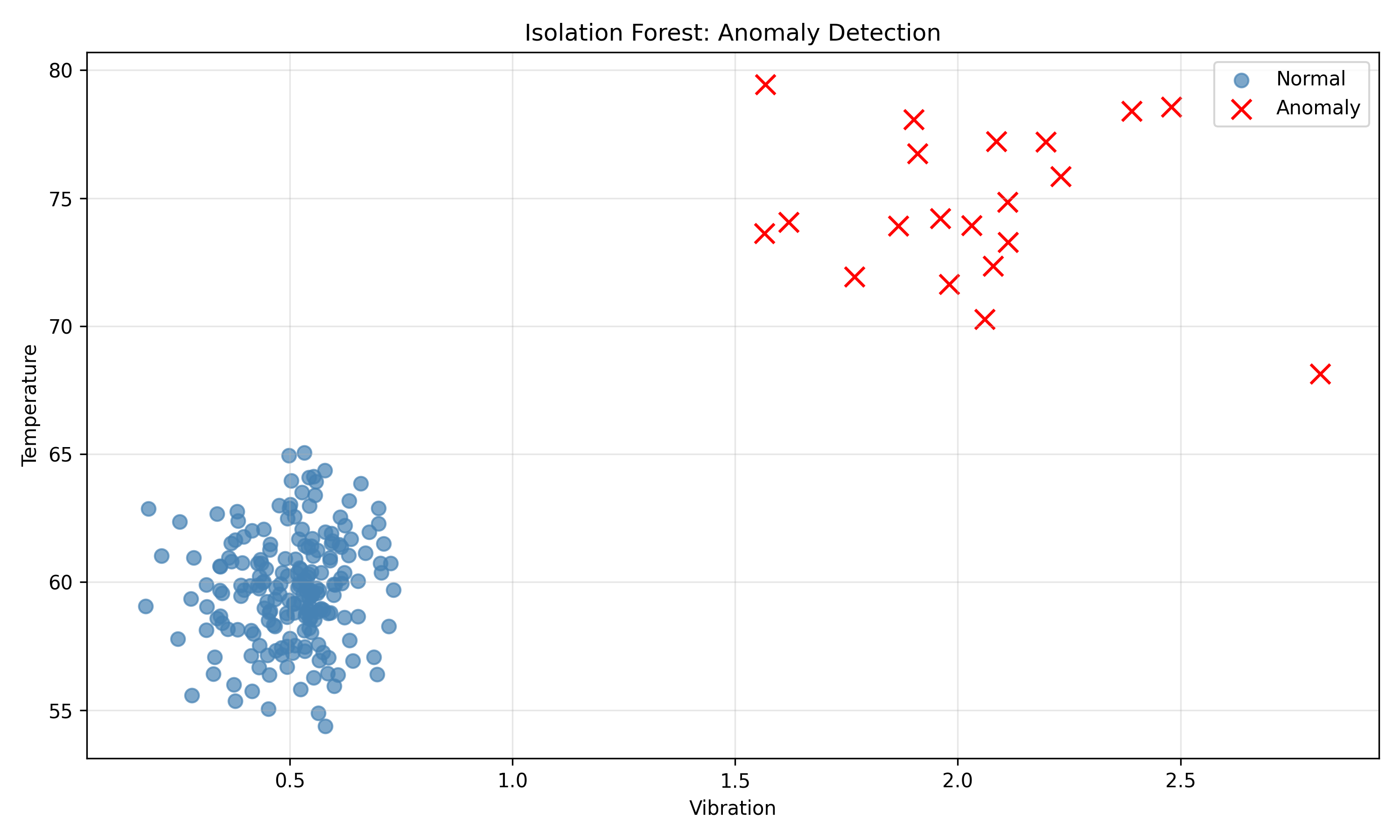
## Anomaly Detection for Early Warning
Even before explicit failure, anomalous sensor patterns can signal trouble. Isolation Forest detects outliers by building isolation trees that separate anomalies (which are rare) from normal data in fewer splits. Autoencoders (neural networks trained to reconstruct their input) flag data points with high reconstruction error as anomalies.
Isolation Forest is simpler and interpretable; autoencoders are more powerful but require more data and tuning.
::: {.callout-tip icon="false"}
## 🔑 Key Formula
$$\text{Isolation Forest Anomaly Score} = 2^{-\frac{E[h(X)]}{c(n)}}$$
where $h(X)$ is the path length in the tree and $c(n)$ is a normalization constant.
:::
::: {.panel-tabset}
## R
```{r}
#| label: ch52-anomaly-detection
library(tidyverse)
library(tidymodels)
library(solitude)
set.seed(6493)
# Generate normal operation data + anomalies
n_normal <- 200
n_anomaly <- 20
normal_data <- tibble(
vibration = rnorm(n_normal, mean = 0.5, sd = 0.1),
temperature = rnorm(n_normal, mean = 60, sd = 2),
current = rnorm(n_normal, mean = 10, sd = 0.5),
anomaly = 0
)
anomaly_data <- tibble(
vibration = rnorm(n_anomaly, mean = 2, sd = 0.3), # High vibration
temperature = rnorm(n_anomaly, mean = 75, sd = 2), # High temp
current = rnorm(n_anomaly, mean = 12, sd = 0.5),
anomaly = 1
)
combined_data <- bind_rows(normal_data, anomaly_data)
# Fit Isolation Forest (solitude package; contamination set via threshold post-fit)
iso_forest <- isolationForest$new(num_trees = 100, sample_size = 32)
iso_forest$fit(combined_data |> select(-anomaly))
# Get anomaly scores via predict()
iso_pred <- iso_forest$predict(combined_data |> select(-anomaly))
iso_scores <- iso_pred$anomaly_score
combined_data$iso_score <- iso_scores
combined_data$is_anomaly <- iso_scores > quantile(iso_scores, 0.95) # top 5% flagged
# Evaluate
tp <- sum((combined_data$is_anomaly == 1) & (combined_data$anomaly == 1))
fp <- sum((combined_data$is_anomaly == 1) & (combined_data$anomaly == 0))
fn <- sum((combined_data$is_anomaly == 0) & (combined_data$anomaly == 1))
precision <- tp / (tp + fp)
recall <- tp / (tp + fn)
cat("\n=== Isolation Forest Anomaly Detection ===\n")
cat("Precision:", round(precision, 3), "\n")
cat("Recall:", round(recall, 3), "\n")
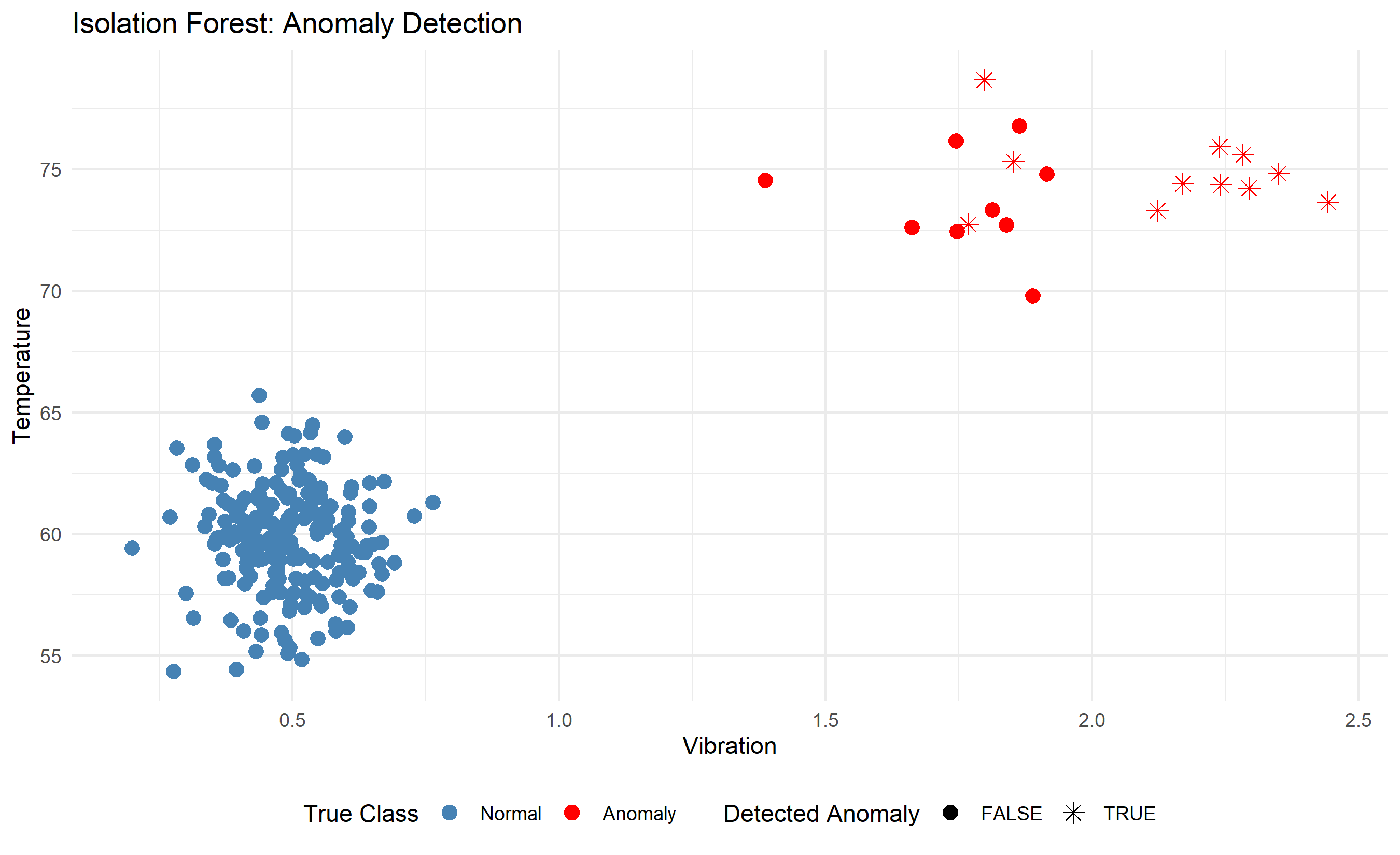
# Visualization
ggplot(combined_data, aes(x = vibration, y = temperature, color = factor(anomaly))) +
geom_point(aes(shape = is_anomaly), size = 3) +
scale_color_manual(values = c("0" = "steelblue", "1" = "red"), labels = c("Normal", "Anomaly")) +
scale_shape_manual(values = c("FALSE" = 16, "TRUE" = 8)) +
labs(
title = "Isolation Forest: Anomaly Detection",
x = "Vibration", y = "Temperature",
color = "True Class", shape = "Detected Anomaly"
) +
theme_minimal() +
theme(legend.position = "bottom")
```
## Python
```{python}
#| label: py-ch52-anomaly-detection
import numpy as np
import pandas as pd
from sklearn.ensemble import IsolationForest
import matplotlib.pyplot as plt
np.random.seed(6493)
# Generate data
normal = np.random.randn(200, 3) * [0.1, 2, 0.5] + [0.5, 60, 10]
anomaly = np.random.randn(20, 3) * [0.3, 2, 0.5] + [2, 75, 12]
X = np.vstack([normal, anomaly])
y_true = np.hstack([np.zeros(200), np.ones(20)])
# Isolation Forest
iso_forest = IsolationForest(contamination=0.05, random_state=6493)
y_pred = iso_forest.fit_predict(X)
scores = iso_forest.score_samples(X)
y_pred = (scores < np.percentile(scores, 5)).astype(int)
# Evaluation
tp = sum((y_pred == 1) & (y_true == 1))
fp = sum((y_pred == 1) & (y_true == 0))
fn = sum((y_pred == 0) & (y_true == 1))
precision = tp / (tp + fp)
recall = tp / (tp + fn)
print("\n=== Isolation Forest Anomaly Detection ===")
print(f"Precision: {precision:.3f}")
print(f"Recall: {recall:.3f}")
# Visualization
fig, ax = plt.subplots(figsize=(10, 6))
scatter = ax.scatter(X[y_true == 0, 0], X[y_true == 0, 1], c='steelblue', label='Normal',
marker='o', s=50, alpha=0.7)
scatter = ax.scatter(X[y_true == 1, 0], X[y_true == 1, 1], c='red', label='Anomaly',
marker='x', s=100)
ax.set_xlabel('Vibration')
ax.set_ylabel('Temperature')
ax.set_title('Isolation Forest: Anomaly Detection')
ax.legend()
ax.grid(True, alpha=0.3)
plt.tight_layout()
plt.show()
```
:::
## Maintenance Scheduling Optimization
Given predicted failure probabilities for 50 machines, maintenance capacity constraints (e.g., 5 technicians, 8 hours/day), and the cost of downtime vs. maintenance, how do you decide which machines to service this week?
This is an integer programming problem. Formulate as:
$$\max \sum_{i=1}^{50} w_i x_i$$
subject to:
$$\sum_{i=1}^{50} t_i x_i \leq T, \quad x_i \in \{0, 1\}$$
where $w_i$ = expected downtime cost avoided for machine $i$, $t_i$ = maintenance time for machine $i$, $T$ = total available maintenance hours, and $x_i = 1$ if machine $i$ is serviced.
::: {.panel-tabset}
## R
```{r}
#| label: ch52-scheduling
library(tidyverse)
library(lpSolve)
set.seed(8271)
# 50 machines with predicted failure probability and maintenance time
n_machines <- 50
machines <- tibble(
machine_id = 1:n_machines,
failure_prob = runif(n_machines, 0.02, 0.5),
downtime_cost_if_fail = 1000 * runif(n_machines, 1, 10),
maintenance_time_hours = runif(n_machines, 1, 8)
)
# Cost avoided by preventive maintenance
machines <- machines |>
mutate(
value = failure_prob * downtime_cost_if_fail
)
cat("\n=== Machines Ranked by Risk ===\n")
machines_ranked <- machines |> arrange(desc(value)) |> head(10)
print(machines_ranked)
# Integer programming: select machines to maximize risk reduction subject to capacity
total_capacity_hours <- 40 # 5 technicians × 8 hours
# Formulate as LP (lpSolve)
c <- machines$value # Objective: maximize value avoided
A_constraint <- matrix(machines$maintenance_time_hours, nrow = 1) # Capacity constraint
b_constraint <- total_capacity_hours
constraint_direction <- "<="
# Solve
result <- lp(
direction = "max",
objective.in = c,
const.mat = A_constraint,
const.dir = constraint_direction,
const.rhs = b_constraint,
all.bin = TRUE # Binary variables
)
# Extract solution
selected_machines <- which(result$solution == 1)
schedule <- machines |>
filter(machine_id %in% selected_machines) |>
arrange(desc(value))
cat("\n=== Maintenance Schedule (This Week) ===\n")
print(schedule[, c("machine_id", "failure_prob", "value", "maintenance_time_hours")])
cat("\nTotal maintenance hours used:", round(sum(schedule$maintenance_time_hours), 1), "\n")
cat("Total risk reduction value:", round(sum(schedule$value), 0), "\n")
cat("Expected downtime cost avoided: ₦", round(sum(schedule$value), 0), "\n")
```
## Python
```{python}
#| label: py-ch52-scheduling
import numpy as np
import pandas as pd
from pulp import *
np.random.seed(8271)
# Create machines
n_machines = 50
machines = pd.DataFrame({
'machine_id': range(1, n_machines + 1),
'failure_prob': np.random.uniform(0.02, 0.5, n_machines),
'downtime_cost_if_fail': 1000 * np.random.uniform(1, 10, n_machines),
'maintenance_time_hours': np.random.uniform(1, 8, n_machines)
})
machines['value'] = machines['failure_prob'] * machines['downtime_cost_if_fail']
print("\n=== Machines Ranked by Risk ===")
print(machines.nlargest(10, 'value'))
# Integer programming
total_capacity_hours = 40 # 5 technicians × 8 hours
prob = LpProblem("Maintenance_Scheduling", LpMaximize)
# Decision variables
x = [LpVariable(f"machine_{i}", cat='Binary') for i in range(n_machines)]
# Objective: maximize risk reduction
prob += lpSum([machines.iloc[i]['value'] * x[i] for i in range(n_machines)])
# Constraint: capacity
prob += lpSum([machines.iloc[i]['maintenance_time_hours'] * x[i] for i in range(n_machines)]) <= total_capacity_hours
# Solve
prob.solve(PULP_CBC_CMD(msg=0))
# Extract solution
selected = [i for i in range(n_machines) if x[i].varValue == 1]
schedule = machines.iloc[selected].sort_values('value', ascending=False)
print("\n=== Maintenance Schedule (This Week) ===")
print(schedule[['machine_id', 'failure_prob', 'value', 'maintenance_time_hours']])
print(f"\nTotal maintenance hours: {schedule['maintenance_time_hours'].sum():.1f}")
print(f"Total risk reduction: ₦{schedule['value'].sum():.0f}")
```
:::
## Case Study: Predictive Maintenance for a Nigerian Cement Plant
A mid-sized Nigerian cement plant operates 50 ball mills. Each mill has 6 sensors (vibration, temperature, pressure, current, bearing oil temp, acoustic emission). Data is collected every 10 minutes. Over 90 days, the plant observes 3 mill failures. We build a complete predictive maintenance system: feature engineering, failure prediction, RUL estimation, anomaly detection, and maintenance scheduling.
::: {.exercises}
#### Chapter 52 Exercises
1. **Feature Importance via SHAP**: Using the failure prediction model from Section 52.3, compute SHAP values for each feature and generate a beeswarm plot showing which sensors are most predictive of failure.
2. **Multi-horizon Forecasting**: Extend the RUL model to predict not just days-to-failure, but also the type of failure (bearing failure, seal failure, misalignment) using a multi-output regression.
3. **Anomaly Detection Benchmark**: Compare Isolation Forest, Local Outlier Factor (LOF), and autoencoder-based anomaly detection on your sensor data. Which detects the pre-failure anomalies earliest?
4. **Maintenance Cost Optimization**: Formulate a multi-week maintenance scheduling problem where decisions in week $t$ depend on predicted states in week $t+1$. Use dynamic programming or rolling-horizon optimization.
5. **Sensor Fusion for RUL**: Combine predictions from multiple sensors (vibration, temperature, oil analysis) into a single RUL estimate using ensemble methods or Bayesian fusion.
:::
## Further Reading
- Vachtsevanos, G., Lewis, F. L., Roemer, M., Hess, A., & Wu, B. (2006). Intelligent fault diagnosis and prognosis for engineering systems. John Wiley & Sons.
- Lei, Y., Yang, B., Jiang, X., Jia, F., Li, N., & Nandi, A. K. (2018). Applications of structural health monitoring in civil structures. Mechanical Systems and Signal Processing, 126, 157–182.
- Bass, R. B., & Alhaj, M. (2022). Remaining useful life estimation for prognostics and health management. Annual Review of Control, Robotics, and Autonomous Systems, 5, 403–427.
## Chapter 52 Appendix: Mathematical Derivations
### A52.1 Discrete Fourier Transform for Vibration Features
For a sampled signal $x[n]$, $n = 0, 1, \ldots, N-1$, the DFT is:
$$X[k] = \sum_{n=0}^{N-1} x[n] e^{-j 2\pi kn/N}$$
The power at frequency bin $k$ is $|X[k]|^2$. For bearing diagnostics, energy in the frequency band containing the ball pass frequency indicates bearing degradation.
### A52.2 Isolation Forest Anomaly Score
An isolation tree randomly selects a feature and split value, partitioning the data. Anomalies (rare) are isolated in fewer splits. The anomaly score for a point $x$ is:
$$s(x, n) = 2^{-\frac{E[h(x)]}{c(n)}}$$
where $h(x)$ is the average path length across trees and $c(n)$ is a normalization constant.
### A52.3 Integer Programming Formulation for Maintenance Scheduling
Maximize:
$$\sum_{i=1}^{n} p_i c_i x_i$$
subject to:
$$\sum_{i=1}^{n} t_i x_i \leq T, \quad x_i \in \{0, 1\}$$
where $p_i$ = predicted failure probability, $c_i$ = downtime cost if machine $i$ fails, $t_i$ = maintenance time, $T$ = total capacity.
---