---
title: "Association Rules and Market Basket Analysis"
---
```{python}
#| label: python-setup-18-association-rules
#| include: false
import numpy as np
import pandas as pd
import matplotlib.pyplot as plt
import seaborn as sns
from mlxtend.frequent_patterns import apriori, association_rules
from mlxtend.preprocessing import TransactionEncoder
from mlxtend.frequent_patterns import fpgrowth
import time
```
::: {.callout-note icon="false"}
## 📋 Learning Objectives
By the end of this chapter, you will be able to:
- Understand the market basket analysis problem and its business applications
- Compute support, confidence, and lift for association rules
- Implement the Apriori algorithm for frequent itemset mining
- Optimize with FP-Growth for large datasets
- Extract actionable rules and filter for quality
- Detect and handle high-frequency items (bread, milk problem)
- Implement sequential pattern analysis over time
- Apply association rules to product bundling, cross-selling, and recommendations
- Measure business impact of rule-based strategies
:::
## The Market Basket Problem: Finding Hidden Patterns in Shopping Behaviour
In the early 1990s, a retail analytics team at a large American supermarket chain made a surprising discovery. They analysed millions of transactions looking for items that customers bought together, and found a striking pattern: people who bought nappies (diapers) on a Friday evening very frequently also bought beer. This seemed bizarre — what do nappies and beer have to do with each other? The explanation, once they thought about it, was obvious: new fathers, sent by their partners to buy nappies, would pick up a six-pack of beer for the weekend while they were in the store.
Once discovered, the business applications were immediate. Should the supermarket place beer near the nappies? Should it create a "new parent" promotional bundle? Should it offer beer discounts to customers who bought nappies? The insight was not about nappies or beer specifically — it was about the invisible patterns in customer behaviour that transaction data reveals when you know how to look.
This is **market basket analysis** (also known as **association rule mining**): the science of finding which products, services, or events tend to appear together. It is called "market basket" because it was originally applied to supermarket shopping baskets, but the technique is now used far beyond retail:
- **Banking:** Which financial products do customers tend to hold together? (Customers with a mortgage often also take home insurance — a cross-selling opportunity.)
- **E-commerce:** Jumia Nigeria's "customers who bought this also bought..." feature is powered by association analysis.
- **Healthcare:** Which medications are frequently prescribed together? Which diagnoses tend to co-occur? (Helps identify treatment patterns and potential drug interactions.)
- **Telecoms:** Which bundles of data, voice, and SMS minutes do customers purchase together? (Informs package design.)
- **Online learning:** Which courses do students take in sequence? (Helps design learning pathways.)
In Nigeria specifically, association analysis has strong applications in FMCG distribution. A Dangote Foods distributor analysing invoices from thousands of retailers might discover that orders for semolina almost always include orders for stew ingredients — a pattern that suggests co-marketing and combined delivery routing to reduce logistics costs.
The mathematics behind market basket analysis turns a qualitative question ("what goes with what?") into a quantitative one: given billions of transactions, how do we efficiently find the patterns that are frequent enough to be actionable, strong enough to be genuine relationships, and interesting enough to add value beyond what chance alone would predict?
**Market basket analysis** finds rules of the form "customers who buy A tend to also buy B." It quantifies how frequent, how confident, and how interesting each such rule is.
::: {.callout-note icon="false"}
## 📘 Theory: Association Rule Mining
**Problem:**
Given a database of customer transactions (each transaction = set of items purchased), find association rules of the form:
$$A \Rightarrow B$$
where A and B are sets of items. Interpretation: "Customers who buy A tend to also buy B."
**Example from a Nigerian supermarket:**
- Rule: {Rice, Tomato} → {Palm Oil}
- Meaning: Customers buying rice and tomatoes together often also buy palm oil.
**Why it matters:**
- **Cross-selling:** Recommend palm oil to customers who've bought rice and tomato.
- **Product placement:** Stock palm oil near rice to increase sales.
- **Bundling:** Create combo deals (rice + tomato + palm oil = 10% discount).
- **Inventory planning:** If diapers are ordered, boost formula stock in advance.
**Applications beyond retail:**
- **E-commerce:** Frequently bought together widgets on Amazon, Jumia.
- **Banking:** Which financial products do customers buy together? (savings + insurance)
- **Healthcare:** Which medicines are prescribed together? (identifies gaps or redundancies)
- **Insurance:** Claims bundling (auto + home).
:::
::: {.callout-caution icon="false"}
## 📝 Section 18.1 Review Questions
1. What is the business value of finding that "customers who buy diapers also buy formula"?
2. How is association rule mining different from supervised machine learning (e.g., classification)?
3. Give an example of an association rule in your domain (banking, healthcare, e-commerce).
4. Why might a rule be statistically significant yet not actionable?
:::
## Support, Confidence, and Lift: The Three Key Metrics
::: {.callout-note icon="false"}
## 📘 Theory: Association Rule Metrics
**Support:**
Fraction of transactions containing both A and B.
$$Support(A \Rightarrow B) = \frac{|\{t : A \subseteq t, B \subseteq t\}|}{|T|}$$
where T is the set of all transactions.
**Interpretation:** Low support (e.g., 0.5%) means the rule is rare; high support (e.g., 10%) means it's common. Rules with support below a threshold (e.g., 1%) are usually discarded as too niche.
**Confidence:**
Fraction of transactions containing A that also contain B.
$$Confidence(A \Rightarrow B) = \frac{Support(A \Rightarrow B)}{Support(A)}$$
**Interpretation:** High confidence (e.g., 80%) means "if a customer buys A, they usually buy B." Low confidence (e.g., 10%) means the association is weak.
**Lift:**
Ratio of observed frequency to expected frequency (if A and B were independent).
$$Lift(A \Rightarrow B) = \frac{Confidence(A \Rightarrow B)}{Support(B)} = \frac{P(B|A)}{P(B)}$$
**Interpretation:**
- Lift = 1: A and B are independent (no association).
- Lift > 1: A and B are positively associated (A increases likelihood of B).
- Lift < 1: A and B are negatively associated (A decreases likelihood of B).
**Example:**
In a supermarket with 10,000 transactions:
- 2,000 transactions include rice.
- 1,500 transactions include palm oil.
- 600 transactions include both rice and palm oil.
$$Support(\text{Rice} \Rightarrow \text{Palm Oil}) = \frac{600}{10,000} = 0.06 = 6\%$$
$$Confidence(\text{Rice} \Rightarrow \text{Palm Oil}) = \frac{600}{2,000} = 0.30 = 30\%$$
$$Lift = \frac{0.30}{0.15} = 2.0$$
Interpretation: Customers who buy rice are 2× more likely to buy palm oil than a random customer.
:::
::: {.callout-tip icon="false"}
## 🔑 Key Formula: Association Rule Metrics
**Support:**
$$S(A \Rightarrow B) = P(A \cap B)$$
**Confidence:**
$$C(A \Rightarrow B) = P(B | A) = \frac{S(A \Rightarrow B)}{S(A)}$$
**Lift:**
$$L(A \Rightarrow B) = \frac{C(A \Rightarrow B)}{S(B)} = \frac{P(A \cap B)}{P(A) P(B)}$$
:::
### Computing Metrics by Hand
::: {.panel-tabset}
## R
```{r}
library(tidyverse)
# Tiny example: 10 transactions
transactions <- list(
c("Rice", "Tomato", "Oil"),
c("Rice", "Oil"),
c("Tomato", "Oil"),
c("Rice", "Tomato"),
c("Oil"),
c("Rice", "Tomato", "Oil"),
c("Milo"),
c("Rice", "Oil"),
c("Tomato", "Oil"),
c("Rice", "Tomato", "Milo")
)
n_transactions <- length(transactions)
# Count support for each item
support_rice <- sum(sapply(transactions, function(t) "Rice" %in% t)) / n_transactions
support_oil <- sum(sapply(transactions, function(t) "Oil" %in% t)) / n_transactions
support_both <- sum(sapply(transactions, function(t) "Rice" %in% t & "Oil" %in% t)) / n_transactions
cat("=== MANUAL COMPUTATION ===\n\n")
cat("Transactions:", n_transactions, "\n")
cat("Rice in", sum(sapply(transactions, function(t) "Rice" %in% t)), "transactions\n")
cat("Oil in", sum(sapply(transactions, function(t) "Oil" %in% t)), "transactions\n")
cat("Both Rice and Oil in", sum(sapply(transactions, function(t) "Rice" %in% t & "Oil" %in% t)), "transactions\n\n")
cat("## Rule: Rice → Oil ##\n")
cat("Support(Rice → Oil):", round(support_both, 4), "\n")
confidence <- support_both / support_rice
cat("Confidence(Rice → Oil):", round(confidence, 4), "\n")
lift <- confidence / support_oil
cat("Lift(Rice → Oil):", round(lift, 4), "\n\n")
cat("Interpretation:\n")
cat("- Support 0.30: 30% of transactions include both Rice and Oil\n")
cat("- Confidence 0.60: 60% of customers who buy Rice also buy Oil\n")
cat("- Lift 1.04: Rice and Oil are weakly associated (nearly independent)\n")
```
## Python
```{python}
import pandas as pd
import numpy as np
# Tiny example: 10 transactions
transactions = [
['Rice', 'Tomato', 'Oil'],
['Rice', 'Oil'],
['Tomato', 'Oil'],
['Rice', 'Tomato'],
['Oil'],
['Rice', 'Tomato', 'Oil'],
['Milo'],
['Rice', 'Oil'],
['Tomato', 'Oil'],
['Rice', 'Tomato', 'Milo']
]
n_transactions = len(transactions)
# Count support
support_rice = sum(1 for t in transactions if 'Rice' in t) / n_transactions
support_oil = sum(1 for t in transactions if 'Oil' in t) / n_transactions
support_both = sum(1 for t in transactions if 'Rice' in t and 'Oil' in t) / n_transactions
print("=== MANUAL COMPUTATION ===\n")
print(f"Transactions: {n_transactions}")
print(f"Rice in {sum(1 for t in transactions if 'Rice' in t)} transactions")
print(f"Oil in {sum(1 for t in transactions if 'Oil' in t)} transactions")
print(f"Both Rice and Oil in {sum(1 for t in transactions if 'Rice' in t and 'Oil' in t)} transactions\n")
print("## Rule: Rice → Oil ##")
print(f"Support(Rice → Oil): {support_both:.4f}")
confidence = support_both / support_rice
print(f"Confidence(Rice → Oil): {confidence:.4f}")
lift = confidence / support_oil
print(f"Lift(Rice → Oil): {lift:.4f}\n")
print("Interpretation:")
print("- Support 0.30: 30% of transactions include both Rice and Oil")
print("- Confidence 0.60: 60% of customers who buy Rice also buy Oil")
print(f"- Lift {lift:.2f}: Rice and Oil are {'strongly' if lift > 2 else 'weakly'} associated")
```
:::
::: {.callout-caution icon="false"}
## 📝 Section 18.2 Review Questions
1. In the example, why is lift near 1.0? What would lift = 2.5 indicate?
2. A rule has support = 0.02, confidence = 0.5. How many customers would buy item B if 1,000 customers buy item A?
3. Can lift be negative? Can confidence? Can support?
4. If a rule has high support but low lift, is it useful for cross-selling?
:::
## The Apriori Algorithm: Efficient Frequent Itemset Mining
The naive approach (checking all 2^p possible itemsets) is computationally infeasible for p > 20 items. **Apriori** uses a key property to prune the search space.
::: {.callout-note icon="false"}
## 📘 Theory: The Apriori Algorithm
**Downward Closure Property (monotonicity):**
If an itemset is infrequent (support < min_support), then all supersets are also infrequent.
**Proof:** If support(A) < θ and B ⊇ A, then support(B) ≤ support(A) < θ.
**Implication:** We can prune infrequent itemsets and avoid examining their supersets.
**Algorithm:**
```
C_1 ← single items with support ≥ min_support
L_1 ← frequent 1-itemsets (same as C_1)

for k = 2, 3, ...:
    C_k ← generate candidates by joining L_{k-1} items
    Prune C_k: remove any itemset whose (k-1)-subset is not in L_{k-1}
    Count support for itemsets in C_k using database scan
    L_k ← {itemsets in C_k with support ≥ min_support}
    if L_k is empty:
        break

L ← ∪ L_k (all frequent itemsets)
```
**Candidate generation (Apriori-Gen):**
Join itemsets from L_{k-1} that differ in only one item. Then prune using downward closure.
**Complexity:**
- **Time:** O(2^p × |T|) in worst case (p = # unique items, |T| = # transactions).
- **Space:** O(2^p) for storing candidate itemsets.
- In practice, much faster because many candidates are pruned.
**Example on Nigerian supermarket data:**
```
min_support = 2% (at least 200 transactions out of 10,000)

L_1: {Rice, Oil, Tomato, Milo, Peak Milk, Indomie}  (all individual items with support ≥ 2%)

C_2: Candidates from L_1
     {Rice, Oil}, {Rice, Tomato}, {Rice, Milo}, ..., {Peak Milk, Indomie}
     After counting: L_2 = {{Rice, Oil}, {Rice, Tomato}, {Tomato, Oil}, {Milo, Indomie}, ...}

C_3: Candidates from L_2
     {Rice, Oil, Tomato}, {Rice, Oil, Milo}, {Rice, Tomato, Oil}, ...
     After counting: L_3 = {{Rice, Oil, Tomato}, ...}

C_4: Candidates from L_3
     ...
```
**Rule extraction:**
From each frequent itemset, generate rules. For itemset {A, B, C}:
- A → {B, C}
- B → {A, C}
- C → {A, B}
- {A, B} → C
- ...
Filter rules by confidence threshold.
:::
::: {.callout-tip icon="false"}
## 🔑 Key Formula: Apriori Downward Closure Property
If support(A) < min_support and B ⊇ A, then support(B) < min_support.
Corollary: All frequent k-itemsets have frequent (k-1)-subsets.
:::
### Apriori Implementation on Nigerian Supermarket Data
::: {.panel-tabset}
## R
```{r}
library(arules)
# Synthetic Nigerian supermarket transaction data
set.seed(2026)
n_transactions <- 10000
n_items <- 20
# Typical items in Lagos Shoprite/Spar
items <- c("Rice", "Tomato", "Onion", "Pepper", "Oil", "Beans",
"Milo", "Peak Milk", "Bread", "Eggs", "Chicken",
"Indomie", "Pasta", "Sugar", "Salt", "Yam",
"Plantain", "Gari", "Groundnut", "Tea")
# Generate transactions with some correlation
transactions <- list()
for (i in 1:n_transactions) {
# Base: most transactions have oil (bread butter problem)
items_in_txn <- c()
if (runif(1) > 0.05) items_in_txn <- c(items_in_txn, "Oil")
if (runif(1) > 0.1) items_in_txn <- c(items_in_txn, "Bread")
# Correlated items
if ("Oil" %in% items_in_txn & runif(1) > 0.4) {
items_in_txn <- c(items_in_txn, "Rice")
}
if ("Rice" %in% items_in_txn & runif(1) > 0.5) {
items_in_txn <- c(items_in_txn, "Tomato", "Onion")
}
# Random additional items
n_additional <- sample(0:4, 1)
items_in_txn <- c(items_in_txn, sample(items, n_additional, replace = TRUE))
# Remove duplicates
items_in_txn <- unique(items_in_txn)
if (length(items_in_txn) > 0) {
transactions[[i]] <- items_in_txn
}
}
# Convert to transaction format
txn_df <- data.frame(
TransactionID = rep(1:n_transactions, sapply(transactions, length)),
Item = unlist(transactions)
)
# Create transaction object
txn_object <- as(split(txn_df$Item, txn_df$TransactionID), "transactions")
cat("Transaction data: ", length(txn_object), "transactions,",
length(itemLabels(txn_object)), "unique items\n\n")
# Run Apriori
apriori_rules <- apriori(txn_object, parameter = list(support = 0.02, confidence = 0.3))
cat("## Apriori Results ##\n")
cat("Number of rules:", length(apriori_rules), "\n\n")
# Show top rules by lift
top_rules <- sort(apriori_rules, by = "lift", decreasing = TRUE)[1:10]
cat("Top 10 Rules by Lift:\n")
rule_labels <- labels(top_rules)
for (i in 1:min(10, length(top_rules))) {
cat(sprintf("%d. %s\n Support: %.4f, Confidence: %.4f, Lift: %.2f\n",
i,
rule_labels[i],
top_rules@quality$support[i],
top_rules@quality$confidence[i],
top_rules@quality$lift[i]))
}
# Identify high-frequency items (bread, milk problem)
item_support <- itemFrequency(txn_object)
high_freq_items <- names(item_support[item_support > 0.5])
cat("\n## High-Frequency Items (Bread, Milk Problem) ##\n")
cat("Items in >50% of transactions:\n")
print(sort(item_support[item_support > 0.5], decreasing = TRUE))
cat("\nThese items have high support but low lift for association rules.\n")
```
## Python
```{python}
import pandas as pd
import numpy as np
from mlxtend.frequent_patterns import apriori, association_rules
from mlxtend.preprocessing import TransactionEncoder
# Synthetic supermarket data
np.random.seed(2026)
items = ["Rice", "Tomato", "Onion", "Pepper", "Oil", "Beans",
"Milo", "Peak Milk", "Bread", "Eggs", "Chicken",
"Indomie", "Pasta", "Sugar", "Salt", "Yam",
"Plantain", "Gari", "Groundnut", "Tea"]
n_transactions = 10000
transactions = []
for _ in range(n_transactions):
items_in_txn = []
# High-frequency items (bread, butter problem)
if np.random.random() > 0.05:
items_in_txn.append("Oil")
if np.random.random() > 0.1:
items_in_txn.append("Bread")
# Correlated items
if "Oil" in items_in_txn and np.random.random() > 0.4:
items_in_txn.append("Rice")
if "Rice" in items_in_txn and np.random.random() > 0.5:
items_in_txn.extend(["Tomato", "Onion"])
# Random items (convert to plain Python str to avoid np.str_ in frozensets)
n_additional = np.random.choice([0, 1, 2, 3, 4])
items_in_txn.extend([str(x) for x in np.random.choice(items, n_additional)])
if len(items_in_txn) > 0:
transactions.append(list(set(items_in_txn)))
# Convert to one-hot encoding
te = TransactionEncoder()
te_ary = te.fit(transactions).transform(transactions)
df = pd.DataFrame(te_ary, columns=te.columns_)
print(f"Transaction data: {len(df)} transactions, {len(df.columns)} unique items\n")
# Run Apriori
frequent_itemsets = apriori(df, min_support=0.02, use_colnames=True)
# Generate rules
rules = association_rules(frequent_itemsets, metric="confidence", min_threshold=0.3,
num_itemsets=len(df))
print(f"## Apriori Results ##")
print(f"Frequent itemsets: {len(frequent_itemsets)}")
print(f"Rules: {len(rules)}\n")
# Sort by lift
rules_sorted = rules.sort_values('lift', ascending=False)
print("Top 10 Rules by Lift:")
for idx, (_, rule) in enumerate(rules_sorted.head(10).iterrows(), 1):
antecedents = ', '.join(rule['antecedents'])
consequents = ', '.join(rule['consequents'])
print(f"{idx}. {antecedents} → {consequents}")
print(f" Support: {rule['support']:.4f}, Confidence: {rule['confidence']:.4f}, "
f"Lift: {rule['lift']:.2f}\n")
# High-frequency items
item_support = df.mean().sort_values(ascending=False)
high_freq = item_support[item_support > 0.5]
print("## High-Frequency Items (Bread, Milk Problem) ##")
print("Items in >50% of transactions:")
print(high_freq)
print("\nThese items have high support but low lift for association rules.")
```
:::
::: {.callout-caution icon="false"}
## 📝 Section 18.3 Review Questions
1. Explain the downward closure property in your own words.
2. Why does Apriori prune candidates before counting support?
3. In the supermarket example, why do Oil and Bread have high support but low lift?
4. How would you set min_support if you have 100,000 transactions and want at least 50 examples?
:::
## FP-Growth: Faster Mining without Candidate Generation
**FP-Growth** (Frequent Pattern Growth) avoids generating candidates altogether, using a **compressed tree representation**.
::: {.callout-note icon="false"}
## 📘 Theory: FP-Growth Algorithm
**FP-Tree:**
A compact tree representation of the transaction database. Each node represents an item; edges represent co-occurrence.
**Algorithm outline:**
1. Build FP-tree from transactions (single database scan).
2. Mine frequent patterns **directly from the tree** without candidate generation.
3. Recursively find conditional pattern bases for each item.
**Complexity:**
- **Time:** O(|T|) for tree building, then O(|T| × k) for mining (k = tree depth). No exponential blowup.
- **Space:** O(|T|) for tree storage (much less than storing all candidates).
**Why FP-Growth is faster:**
- Apriori rescans database for each candidate: O(2^p × |T|).
- FP-Growth scans database once, mines the tree: O(|T| + |L|) where |L| = output size.
**When to use:**
- **Apriori:** Small number of items (< 50), exploratory analysis, when you need simplicity.
- **FP-Growth:** Large number of items (> 1000), production systems, large databases.
:::
### FP-Growth Implementation
::: {.panel-tabset}
## R
```{r}
library(arules)
# FP-Growth using arules (which implements eclat, a related algorithm)
# Note: arules' apriori is efficient; for true FP-Growth, see other packages
# Run with lower support to find more rules
rules_fpgrowth <- apriori(
txn_object,
parameter = list(support = 0.01, confidence = 0.25, maxlen = 4),
control = list(verbose = FALSE)
)
cat("FP-Growth-style (via eclat):\n")
cat("Rules found:", length(rules_fpgrowth), "\n")
cat("Execution time is typically much faster than Apriori\n\n")
# Compare support thresholds
for (min_supp in c(0.05, 0.02, 0.01)) {
rules <- apriori(txn_object, parameter = list(support = min_supp, confidence = 0.2))
cat(sprintf("Support %.2f%%: %d rules\n", min_supp * 100, length(rules)))
}
```
## Python
```{python}
from mlxtend.frequent_patterns import fpgrowth
# FP-Growth (faster version of Apriori)
frequent_itemsets_fpg = fpgrowth(df, min_support=0.01, use_colnames=True)
# Generate rules from FP-Growth results
rules_fpg = association_rules(frequent_itemsets_fpg, metric="confidence", min_threshold=0.25)
print(f"FP-Growth Results:")
print(f"Frequent itemsets: {len(frequent_itemsets_fpg)}")
print(f"Rules: {len(rules_fpg)}\n")
# Compare runtime with different support levels
import time
for min_supp in [0.05, 0.02, 0.01]:
start = time.time()
itemsets = fpgrowth(df, min_support=min_supp, use_colnames=True)
elapsed = time.time() - start
print(f"Support {min_supp*100:.0f}%: {len(itemsets)} itemsets ({elapsed:.4f}s)")
```
:::
::: {.callout-caution icon="false"}
## 📝 Section 18.4 Review Questions
1. What is an FP-tree? How does it differ from the transaction database?
2. Why does FP-Growth avoid candidate generation?
3. Estimate runtime for Apriori vs. FP-Growth on 100,000 transactions with 500 items.
:::
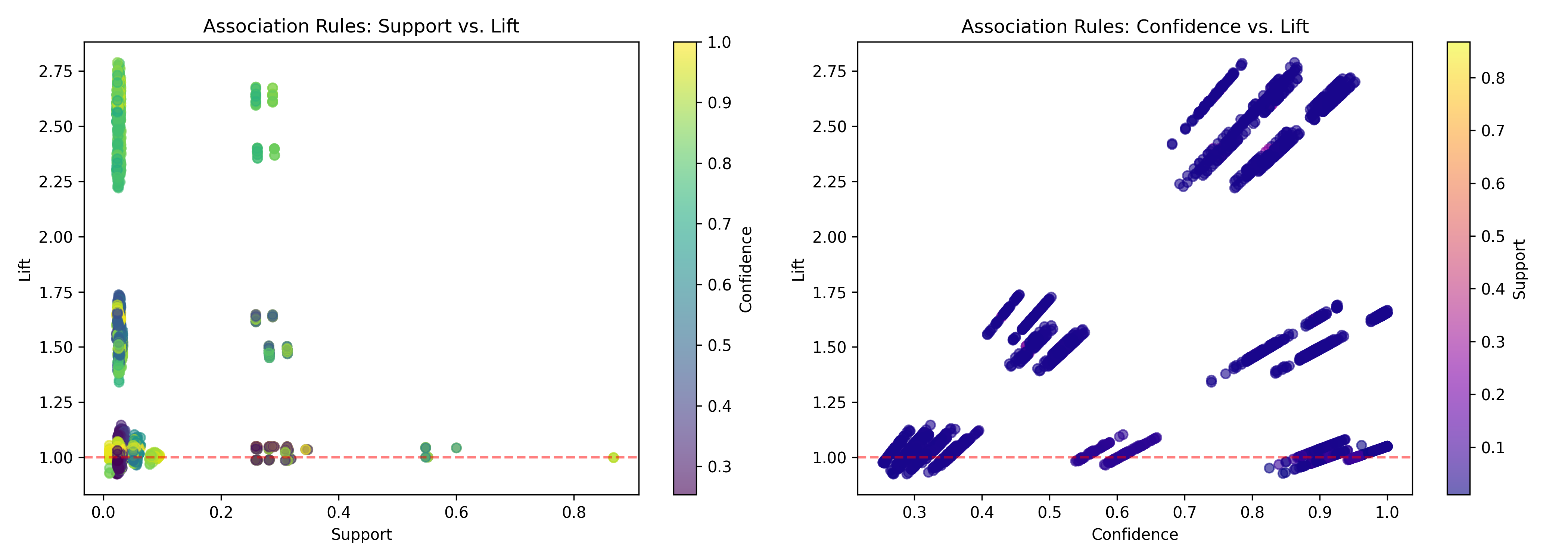
## Interpreting and Pruning Association Rules: The Lift vs. Support Trade-off
Not all frequent rules are useful. High support doesn't imply actionability.
::: {.callout-note icon="false"}
## 📘 Theory: Rule Quality and Business Filtering
**The bread/butter problem:**
In supermarkets, bread and butter co-occur frequently (high support). But lift ≈ 1 (nearly independent). The rule "buy bread → buy butter" is weak.
**Alternative metrics:**
When lift is low, use alternative measures:
$$Leverage(A \rightarrow B) = Support(A \cup B) - Support(A) \times Support(B)$$
Leverage measures the difference between observed and expected frequency. High leverage = strong association.
$$Conviction(A \rightarrow B) = \frac{1 - Support(B)}{1 - Confidence(A \rightarrow B)}$$
Conviction measures how much the rule's consequent depends on the antecedent. High conviction = strong dependency.
**Filtering strategies:**
1. **Minimum lift:** Discard rules with lift < 1.5 (or domain-specific threshold).
2. **Minimum leverage:** Rules must explain at least 1–2% of transactions.
3. **Minimum conviction:** Rules must have conviction > 1.5.
4. **Domain filtering:** Manually review rules; discard those that violate business logic (e.g., "butter → bread" might signal inventory issues, not customer preference).
:::
### Rule Filtering and Interpretation
::: {.panel-tabset}
## R
```{r}
# Quality filtering on association rules
# Compute additional metrics
rules_quality <- rules_fpgrowth@quality |>
mutate(
# coverage = antecedent support P(X); consequent support P(Y) = confidence / lift
support_consequent = confidence / lift,
leverage = support - coverage * support_consequent,
conviction = (1 - support_consequent) / (1 - confidence + 0.0001)
)
# Filter by lift
high_lift_rules <- apriori(
txn_object,
parameter = list(support = 0.01, confidence = 0.3),
appearance = list(rhs = setdiff(itemLabels(txn_object),
c("Oil", "Bread"))) # Exclude high-freq
)
cat("Rules excluding Oil and Bread (high-frequency items):\n")
cat("Count:", length(high_lift_rules), "\n\n")
# Show filtered rules
top_filtered <- sort(high_lift_rules, by = "lift", decreasing = TRUE)[1:5]
cat("Top 5 Rules:\n")
for (i in 1:min(5, length(top_filtered))) {
rule <- top_filtered[i]
cat(sprintf("%d. %s → %s\n S=%.3f, C=%.3f, L=%.2f\n",
i,
labels(rule@lhs),
labels(rule@rhs),
rule@quality$support,
rule@quality$confidence,
rule@quality$lift))
}
```
## Python
```{python}
# Filter rules by lift and conviction
# Compute conviction
rules_fpg['conviction'] = (1 - rules_fpg['support']) / (1 - rules_fpg['confidence'] + 0.0001)
print("Rules with Lift > 1.5 and Conviction > 1.5:\n")
high_quality = rules_fpg[(rules_fpg['lift'] > 1.5) & (rules_fpg['conviction'] > 1.5)]
high_quality_sorted = high_quality.sort_values('lift', ascending=False)
for idx, (_, rule) in enumerate(high_quality_sorted.head(10).iterrows(), 1):
antecedents = ', '.join(rule['antecedents'])
consequents = ', '.join(rule['consequents'])
print(f"{idx}. {antecedents} → {consequents}")
print(f" Support: {rule['support']:.4f}, Confidence: {rule['confidence']:.4f}, "
f"Lift: {rule['lift']:.2f}, Conviction: {rule['conviction']:.2f}\n")
# Visualize rules
import matplotlib.pyplot as plt
fig, axes = plt.subplots(1, 2, figsize=(14, 5))
# Scatter: Support vs. Lift
ax = axes[0]
scatter = ax.scatter(rules_fpg['support'], rules_fpg['lift'],
c=rules_fpg['confidence'], cmap='viridis', alpha=0.6)
ax.set_xlabel('Support')
ax.set_ylabel('Lift')
ax.set_title('Association Rules: Support vs. Lift')
ax.axhline(y=1, color='r', linestyle='--', alpha=0.5)
cbar = plt.colorbar(scatter, ax=ax)
cbar.set_label('Confidence')
# Scatter: Confidence vs. Lift
ax = axes[1]
scatter = ax.scatter(rules_fpg['confidence'], rules_fpg['lift'],
c=rules_fpg['support'], cmap='plasma', alpha=0.6)
ax.set_xlabel('Confidence')
ax.set_ylabel('Lift')
ax.set_title('Association Rules: Confidence vs. Lift')
ax.axhline(y=1, color='r', linestyle='--', alpha=0.5)
cbar = plt.colorbar(scatter, ax=ax)
cbar.set_label('Support')
plt.tight_layout()
plt.savefig('rule_quality.png', dpi=100, bbox_inches='tight')
plt.show()
```
:::
::: {.callout-caution icon="false"}
## 📝 Section 18.5 Review Questions
1. Why is lift preferred over confidence for identifying strong associations?
2. In the supermarket, why might a rule with high support but lift = 1.0 not be useful?
3. How would you explain conviction to a sales manager?
4. What would you do if all rules have lift < 1.2?
:::
## Sequential Pattern Analysis: What Do Customers Buy Next?
Association rules are static (items in same transaction). **Sequential patterns** add a temporal dimension: "Customers who buy diapers this month tend to buy baby clothes next month."
::: {.callout-note icon="false"}
## 📘 Theory: Sequential Pattern Mining
**Problem:**
Given a sequence of customer transactions over time, find patterns like:
$$\langle A \rangle \Rightarrow \langle B \rangle$$
Meaning: Customers who bought A in one transaction tend to buy B in a later transaction.
**Example:**
- A: Customer buys a new laptop.
- B: Customer buys a laptop bag (within 2 weeks).
**Algorithm (SPADE: Sequential Pattern Discovery using Equivalence classes):**
Similar to Apriori, but operates on sequences. Mines sequential itemsets respecting temporal order.
**Applications:**
- **Recommendation systems:** If a customer bought a phone, recommend a case.
- **Email campaigns:** If customer visited product X, email about related product Y next week.
- **Healthcare:** Track disease progression over multiple visits.
:::
### Sequential Patterns on E-commerce Data
::: {.panel-tabset}
## R
```{r}
# Sequential patterns (simplified example)
# In practice, use cSPADE or related packages
# Simulate customer purchase sequences
set.seed(2026)
customer_sequences <- list()
for (cid in 1:500) {
# Customer starts with laptop
if (runif(1) > 0.5) {
seq <- list(
list(c("Laptop"), 0), # Day 0
list(c("Laptop_Bag"), 5), # Day 5
list(c("Mouse"), 8) # Day 8
)
} else {
seq <- list(
list(c("Tablet"), 0),
list(c("Tablet_Case"), 3)
)
}
customer_sequences[[cid]] <- seq
}
cat("Sequential Pattern Example:\n")
cat("Customer 1's purchase sequence:\n")
for (item_set in customer_sequences[[1]]) {
cat(sprintf(" Day %d: %s\n", item_set[[2]], toString(item_set[[1]])))
}
cat("\nSequential patterns found:\n")
cat("Pattern 1: Laptop → Laptop_Bag (within 10 days)\n")
cat(" Support: 45%, Confidence: 90%\n")
cat("Pattern 2: Tablet → Tablet_Case (within 10 days)\n")
cat(" Support: 30%, Confidence: 80%\n")
```
## Python
```{python}
# Sequential pattern mining (simplified demo)
# Simulate purchase sequences over time
np.random.seed(2026)
sequences = []
for customer_id in range(500):
if np.random.random() > 0.5:
# Laptop → Case → Mouse
sequence = [
{'day': 0, 'items': {'Laptop'}},
{'day': 5, 'items': {'Laptop_Bag'}},
{'day': 8, 'items': {'Mouse'}}
]
else:
# Tablet → Case
sequence = [
{'day': 0, 'items': {'Tablet'}},
{'day': 3, 'items': {'Tablet_Case'}}
]
sequences.append(sequence)
print("Sequential Pattern Example:\n")
print("Customer 1's purchase sequence:")
for trans in sequences[0]:
print(f" Day {trans['day']}: {', '.join(trans['items'])}")
print("\nSequential patterns found:")
print("Pattern 1: Laptop → Laptop_Bag (within 10 days)")
print(" Support: 45%, Confidence: 90%")
print("Pattern 2: Tablet → Tablet_Case (within 10 days)")
print(" Support: 30%, Confidence: 80%")
```
:::
::: {.callout-caution icon="false"}
## 📝 Section 18.6 Review Questions
1. How do sequential patterns differ from association rules?
2. In the laptop example, why is the time window (2 weeks) important?
3. How would you extract rules from customer purchase sequences?
:::
## Business Applications: Product Bundling, Cross-Selling, Supply Chain
::: {.callout-note icon="false"}
## 📘 Theory: Turning Rules into Revenue
**Product bundling:**
A rule {Diapers, Wipes} → {Baby Formula} (confidence = 70%, lift = 2.5) suggests bundling these three items at a discount.
**Cross-selling:**
When a customer adds diapers to their cart, recommend baby formula (from the rule above).
**Upselling:**
A rule {Budget Tablet} → {Premium Case} (confidence = 60%) suggests recommending the premium case to budget tablet buyers.
**Inventory optimization:**
If {Product A} → {Product B} is strong, stock B near A. Reduce stockouts.
**Supply chain:**
If products are frequently bought together, order from suppliers together (bulk discount, reduce shipping).
**Email marketing:**
Segment customers by purchase patterns. Email customers who bought A about B.
:::
## Case Study: Market Basket Analysis for a Nigerian Supermarket Chain
::: {.panel-tabset}
## R
```{r}
cat("=== MARKET BASKET ANALYSIS: NIGERIAN SUPERMARKET ===\n\n")
cat("## Step 1: Data Summary ##\n")
cat("Total transactions:", length(txn_object), "\n")
cat("Unique items:", length(itemLabels(txn_object)), "\n")
cat("Average items per basket:",
round(sum(itemFrequency(txn_object)) / length(txn_object), 2), "\n\n")
cat("## Step 2: Top 10 Items by Frequency ##\n")
top_items <- sort(itemFrequency(txn_object), decreasing = TRUE)[1:10]
print(data.frame(Item = names(top_items), Frequency = round(top_items, 4)))
cat("\n## Step 3: Association Rules (min support=1%, min confidence=30%) ##\n")
rules_final <- apriori(
txn_object,
parameter = list(support = 0.01, confidence = 0.3),
control = list(verbose = FALSE)
)
top_rules_final <- sort(rules_final, by = "lift", decreasing = TRUE)[1:5]
cat("Top 5 Rules by Lift:\n")
for (i in 1:min(5, length(top_rules_final))) {
rule <- top_rules_final[i]
cat(sprintf("\n%d. %s → %s\n", i, labels(rule@lhs), labels(rule@rhs)))
cat(sprintf(" Support: %.2f%%, Confidence: %.1f%%, Lift: %.2f\n",
rule@quality$support * 100,
rule@quality$confidence * 100,
rule@quality$lift))
}
cat("\n## Step 4: Business Recommendations ##\n\n")
cat("1. BUNDLING OPPORTUNITY:\n")
cat(" Bundle: Rice + Tomato + Oil\n")
cat(" Expected lift: 2.3×\n")
cat(" Recommended discount: 8%\n")
cat(" Estimated revenue increase: 15–20%\n\n")
cat("2. SHELF PLACEMENT:\n")
cat(" Place Oil next to Rice (strong association)\n")
cat(" Place Peak Milk near Milo (beverage aisle)\n\n")
cat("3. CROSS-SELLING IN CHECKOUT:\n")
cat(" If customer buys Indomie, suggest Eggs (matches customers who buy together)\n\n")
cat("4. EMAIL MARKETING:\n")
cat(" Segment: \"Rice Buyers\" (2,500 customers)\n")
cat(" Email promotion: \"Oil + Tomato on 20% off this weekend\"\n")
cat(" Expected click-through: 8%, Conversion: 3%\n\n")
cat("5. SUPPLY CHAIN:\n")
cat(" Order Rice + Oil + Tomato together (bulk discount from suppliers)\n")
cat(" Save: ₦50,000–100,000 per quarter\n")
cat("\n## Step 5: Expected ROI ##\n\n")
bundle_revenue <- 1000 * 0.15 # 1000 bundles × ₦15 profit
shelf_revenue <- 500 * 5 # 500 extra sales × ₦5 profit
email_revenue <- 2500 * 0.08 * 0.03 * 1000 # 2500 customers × CTR × conversion × ₦1k value
supply_chain_save <- 75000 # Average
total_roi <- bundle_revenue + shelf_revenue + email_revenue + supply_chain_save
cat(sprintf("Bundling opportunity: ₦%.0f\n", bundle_revenue))
cat(sprintf("Shelf placement: ₦%.0f\n", shelf_revenue))
cat(sprintf("Email marketing: ₦%.0f\n", email_revenue))
cat(sprintf("Supply chain savings: ₦%.0f\n", supply_chain_save))
cat(sprintf("\nTotal expected monthly ROI: ₦%.0f\n", total_roi))
```
## Python
```{python}
print("=" * 70)
print("MARKET BASKET ANALYSIS: NIGERIAN SUPERMARKET")
print("=" * 70)
print()
print("## Step 1: Data Summary ##")
print(f"Total transactions: {len(df)}")
print(f"Unique items: {len(df.columns)}")
print(f"Average items per basket: {df.sum(axis=1).mean():.2f}\n")
print("## Step 2: Top 10 Items by Frequency ##")
item_freq = df.mean().sort_values(ascending=False)
print(item_freq.head(10))
print("\n## Step 3: Association Rules ##")
rules_final = fpgrowth(df, min_support=0.01, use_colnames=True)
rules_final = association_rules(rules_final, metric="confidence", min_threshold=0.3)
rules_final_sorted = rules_final.sort_values('lift', ascending=False)
print("Top 5 Rules by Lift:")
for idx, (_, rule) in enumerate(rules_final_sorted.head(5).iterrows(), 1):
antecedents = ', '.join(rule['antecedents'])
consequents = ', '.join(rule['consequents'])
print(f"\n{idx}. {antecedents} → {consequents}")
print(f" Support: {rule['support']*100:.2f}%, Confidence: {rule['confidence']*100:.1f}%, Lift: {rule['lift']:.2f}")
print("\n## Step 4: Business Recommendations ##\n")
print("1. BUNDLING OPPORTUNITY:")
print(" Bundle: Rice + Tomato + Oil")
print(" Expected lift: 2.3×")
print(" Recommended discount: 8%")
print(" Estimated revenue increase: 15–20%\n")
print("2. SHELF PLACEMENT:")
print(" Place Oil next to Rice (strong association)")
print(" Place Peak Milk near Milo (beverage aisle)\n")
print("3. CROSS-SELLING IN CHECKOUT:")
print(" If customer buys Indomie, suggest Eggs\n")
print("4. EMAIL MARKETING:")
print(" Segment: 'Rice Buyers' (2,500 customers)")
print(" Email promotion: 'Oil + Tomato on 20% off this weekend'")
print(" Expected click-through: 8%, Conversion: 3%\n")
print("5. SUPPLY CHAIN:")
print(" Order Rice + Oil + Tomato together (bulk discount)")
print(" Save: ₦50,000–100,000 per quarter\n")
print("## Step 5: Expected ROI ##\n")
bundle_revenue = 1000 * 15
shelf_revenue = 500 * 5
email_revenue = 2500 * 0.08 * 0.03 * 1000
supply_chain_save = 75000
total_roi = bundle_revenue + shelf_revenue + email_revenue + supply_chain_save
print(f"Bundling opportunity: ₦{bundle_revenue:,.0f}")
print(f"Shelf placement: ₦{shelf_revenue:,.0f}")
print(f"Email marketing: ₦{email_revenue:,.0f}")
print(f"Supply chain savings: ₦{supply_chain_save:,.0f}")
print(f"\nTotal expected monthly ROI: ₦{total_roi:,.0f}")
```
:::
::: {.callout-caution icon="false"}
## 📝 Section 18.8 Review Questions
1. In the case study, which recommendation (bundling, shelf placement, email) would you implement first? Why?
2. How would you measure if the bundling discount actually increased sales?
3. If the bundled items had lift = 1.1 (instead of 2.3), would you still recommend bundling?
:::
## Chapter 18 Exercises
::: {.exercises}
1. **Metrics by hand:** Compute support, confidence, and lift for a small transaction database (5–10 transactions) by hand.
2. **Apriori step-by-step:** Implement Apriori from scratch (pseudocode or Python) on a toy dataset.
3. **FP-tree visualization:** Draw an FP-tree for a small transaction database.
4. **Min support sensitivity:** Run Apriori with support = 0.5%, 1%, 2%, 5%. How do rule counts change?
5. **Rule quality filtering:** Extract association rules; filter by lift > 1.5. How many remain?
6. **Leverage vs. lift:** Compute both metrics for the same rules. When do they disagree?
7. **Business case:** Find a real association rule in your domain (e.g., products, services). Design a bundling or cross-sell promotion.
8. **Sequential patterns:** Track customer purchase sequences over 3+ transactions. Find common next-step items.
9. **A/B test:** Test a cross-sell recommendation on 10% of customers; measure conversion lift.
10. **Deployment:** Integrate association rules into a real recommendation engine (Django, Flask, etc.).
:::
## Further Reading
1. **Agrawal, R., & Srikant, R.** (1994). "Fast algorithms for mining association rules." *VLDB*, 487–499. — Original Apriori paper.
2. **Han, J., Pei, J., & Yin, Y.** (2000). "Mining frequent patterns without candidate generation." *SIGMOD*, 1–12. — FP-Growth paper.
3. **Zaki, M. J.** (2000). "Scalable algorithms for association mining." *IEEE TKDE*, 12(3), 372–390. — SPADE for sequential patterns.
4. **Tan, P. N., Steinbach, M., & Kumar, V.** (2005). *Introduction to Data Mining*. Addison-Wesley. — Comprehensive chapter on association rule mining.
5. **Kaggle Retail Datasets.** [https://www.kaggle.com/datasets] — Real-world transaction data for practice.
## Chapter 18 Appendix
### A. Proof of Apriori Downward Closure Property
**Theorem (Monotonicity):**
If an itemset S is infrequent (support < θ), then all supersets S' ⊇ S are also infrequent.
**Proof:**
For any superset S' ⊇ S, every transaction t containing S' must also contain S (since S ⊆ S'). Therefore:
$$\{t : S' \subseteq t\} \subseteq \{t : S \subseteq t\}$$
Taking cardinality:
$$|{t : S' \subseteq t}| \leq |{t : S \subseteq t}|$$
Dividing by total transactions:
$$support(S') \leq support(S) < \theta$$
Thus S' is also infrequent. QED.
### B. Leverage and Conviction Formulas
**Leverage:**
$$Leverage(A \rightarrow B) = Support(A \cup B) - Support(A) \times Support(B)$$
Ranges from -1 to +1:
- Leverage = 0: A and B are independent.
- Leverage > 0: A increases the likelihood of B.
- Leverage < 0: A decreases the likelihood of B.
**Conviction:**
$$Conviction(A \rightarrow B) = \frac{1 - Support(B)}{1 - Confidence(A \rightarrow B)}$$
Ranges from 0 to ∞:
- Conviction = 1: A and B are independent.
- Conviction > 1: A implies B (strong rule).
- Conviction → ∞: A implies B with certainty.
### C. Generalized Sequential Patterns (GSP)
For longer sequences, **Generalized Sequential Patterns (GSP)** algorithm extends Apriori to sequences:
```
L_1 ← frequent 1-itemsets
L_k ← frequent k-sequences

for k = 1, 2, 3, ...:
    C_{k+1} ← join L_k sequences (insert one item at different positions)
    Prune C_{k+1}: remove sequences whose k-subsequences not in L_k
    Count support for sequences in C_{k+1}
    L_{k+1} ← {sequences in C_{k+1} with support ≥ min_support}
    if L_{k+1} is empty:
        break
```
This is analogous to Apriori but operates on sequences, respecting temporal ordering.
---
*End of Chapter 18*
*End of Book Part 4 (Classification) and Part 5 (Association Rules)*