---
title: "Neural Networks: An Accessible Introduction"
author: "Bongo Adi"
---
```{python}
#| label: python-setup-33-neural-networks
#| include: false
import numpy as np
import pandas as pd
import matplotlib.pyplot as plt
import seaborn as sns
from sklearn.metrics import roc_auc_score, roc_curve
from sklearn.linear_model import LogisticRegression
```
::: {.callout-note icon="false"}
## 📋 Learning Objectives
- Understand the biological inspiration and mathematical formulation of artificial neurons
- Build and train feedforward neural networks from first principles using matrix algebra
- Apply backpropagation to optimise network weights on real data
- Recognise when neural networks are the appropriate tool versus simpler alternatives
- Implement a complete neural network pipeline on Nigerian telecom churn data
:::
## The Biological Analogy and Beyond
The story of artificial neural networks begins not in a computer science lab, but in the neuroscience of the 1940s. Warren McCulloch and Walter Pitts observed that biological neurons operate as thresholding devices: they receive signals through dendrites from other neurons, integrate those signals in the cell body, and fire an electrical impulse down the axon if the cumulative signal exceeded a threshold. This observation—that a neuron was fundamentally a threshold function—led to a beautiful mathematical abstraction: the artificial neuron. However, it is crucial to understand that the analogy, while pedagogically useful, is limited. Real neurons are far more complex: they communicate through chemical synapses with variable efficacy, their firing rate depends on temporal patterns of input, they exhibit plasticity over days and weeks, and they operate in networks that exploit feedback loops, neuromodulators, and mechanisms we still do not fully understand. The artificial neuron is a caricature—a drastic simplification that captures one essential idea (integration and thresholding) and discards almost everything else. We use it anyway because, despite its crudeness, it works.
The practical history of neural networks is one of cycles of hype and disappointment. Frank Rosenblatt introduced the perceptron in 1957, a single-layer network that could learn a linear decision boundary. For years, researchers dreamed of stacking layers to build deeper networks. That dream collided with a mathematical wall in the 1970s and 1980s: the vanishing gradient problem. When you tried to train deep networks by backpropagation (the algorithm for computing weight gradients), the gradients flowing backward through many layers would shrink exponentially, becoming so small that learning in the early layers stalled. The field retreated. Support vector machines, random forests, and kernel methods became fashionable. Then, between 2011 and 2012, three breakthroughs converged: GPUs made it cheap to train large networks in hours instead of months, massive datasets became available (ImageNet had 14 million labelled images by 2010), and researchers—Hinton, Bengio, LeCun, and others—discovered that ReLU activations and careful weight initialisation largely sidestepped the vanishing gradient problem. The 2012 ImageNet competition saw a convolutional neural network (AlexNet) vastly outperform traditional computer vision methods, and the deep learning renaissance began. Today, neural networks drive language models, computer vision, speech recognition, and play dominoes.
## The Artificial Neuron
At the heart of every neural network sits the artificial neuron: a function that takes multiple numeric inputs, weights them, sums them, adds a bias, and passes the result through an activation function. Mathematically, given inputs $x_1, x_2, \ldots, x_n$, weights $w_1, w_2, \ldots, w_n$, and bias $b$, we compute the pre-activation value (or "logit") as:
$$z = w_1 x_1 + w_2 x_2 + \cdots + w_n x_n + b = \mathbf{w}^T \mathbf{x} + b$$
We then apply an activation function $f$ to introduce nonlinearity:
$$a = f(z)$$
The output $a$ becomes the input to the next layer. Without the activation function—if $f$ were the identity function—stacking layers would be pointless because the composition of linear functions is linear, and a multi-layer network would compute no more than a single linear transformation. Activation functions are what give neural networks their expressive power.
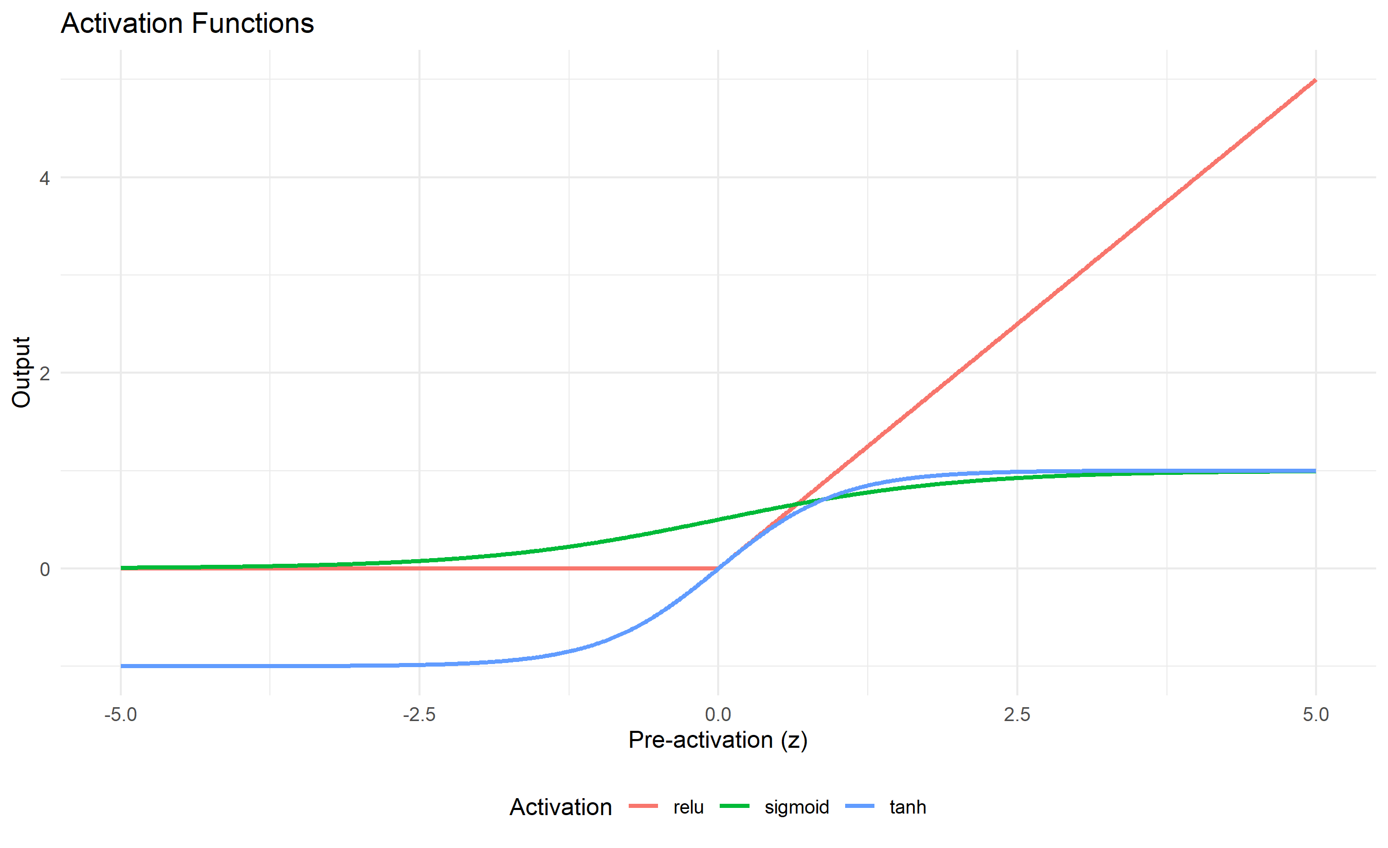
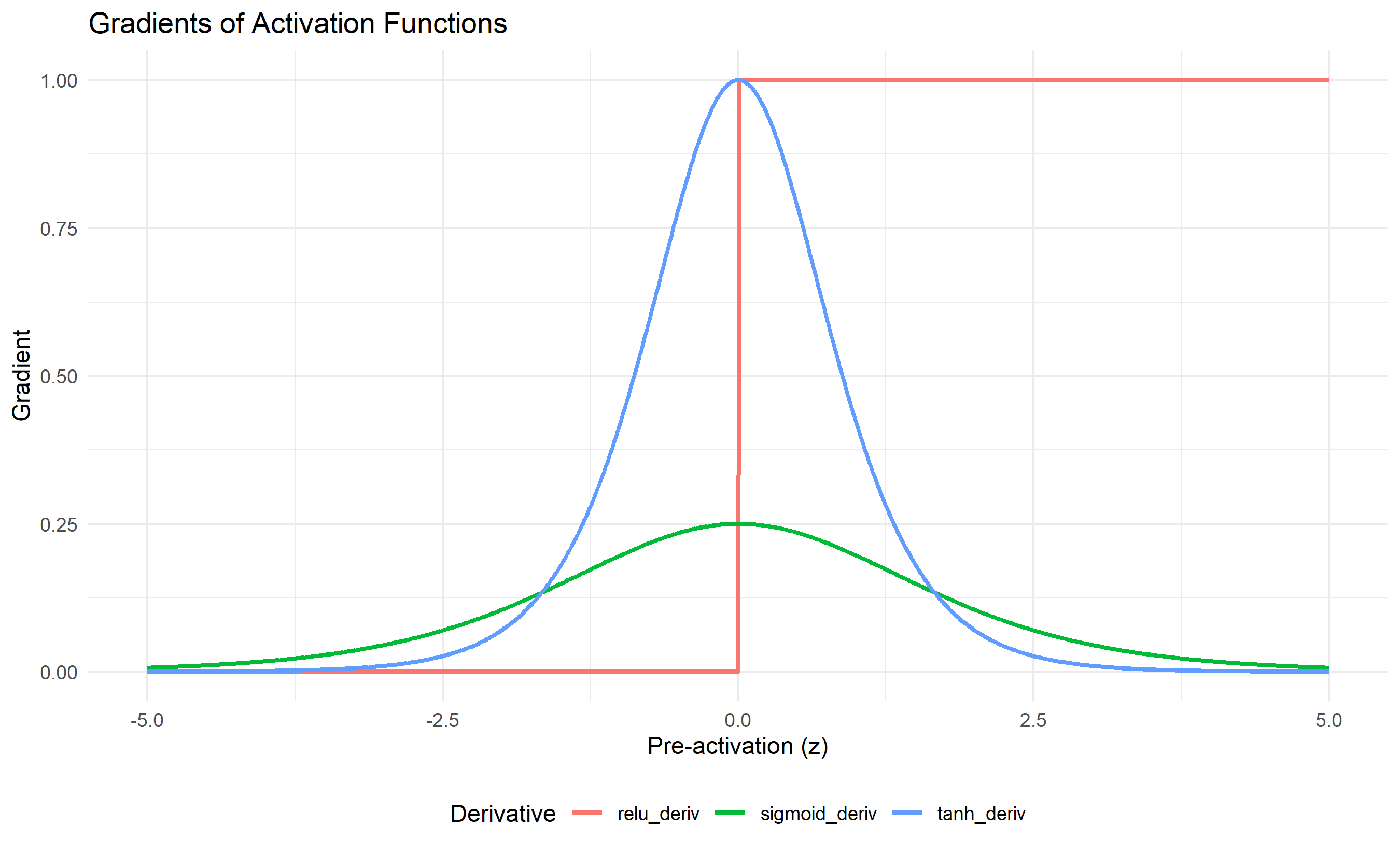
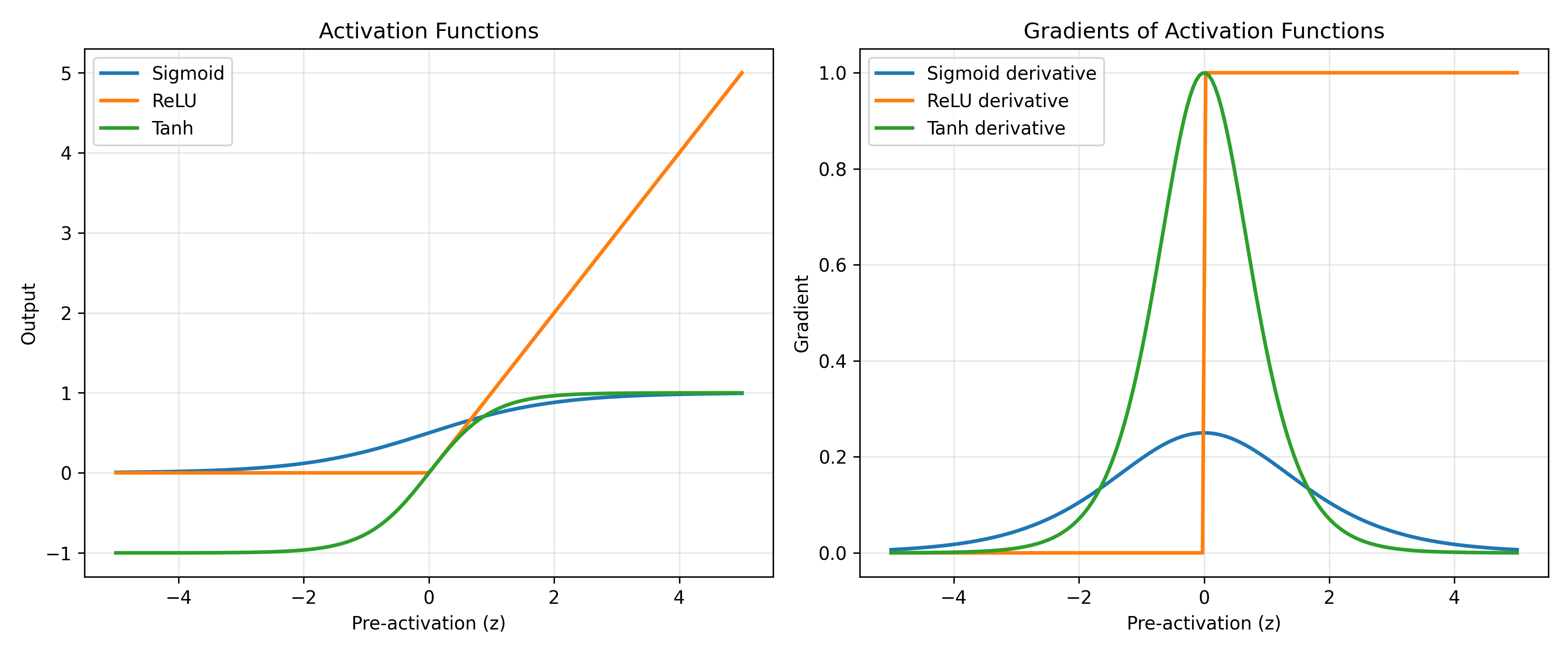
The sigmoid activation function, $\sigma(z) = \frac{1}{1 + e^{-z}}$, was historically the standard. It maps any input to the range $(0, 1)$, making it natural for binary classification (interpret the output as a probability). However, sigmoid has a sharp peak in its derivative around $z = 0$, meaning gradients are tiny except in a narrow region. This exacerbates the vanishing gradient problem in deep networks. The hyperbolic tangent, $\tanh(z) = \frac{e^z - e^{-z}}{e^z + e^{-z}}$, maps to $(-1, 1)$ and has a steeper gradient than sigmoid, making it slightly better for hidden layers. Today, the Rectified Linear Unit (ReLU), defined as $f(z) = \max(0, z)$, dominates hidden layers. It is simple to compute, its gradient is a constant 1 for positive inputs, and it naturally gives rise to sparse activations (many neurons output exactly zero). For multi-class classification, the softmax function normalises a vector of logits into a probability distribution: given logits $z_1, \ldots, z_K$ for $K$ classes, softmax outputs
$$p_k = \frac{e^{z_k}}{\sum_{j=1}^K e^{z_j}}$$
Each $p_k$ is between 0 and 1, and they sum to 1, so we can interpret them as class probabilities.
::: {.callout-note icon="false"}
## 📘 Theory: Activation Functions and Their Properties
:::
::: {.callout-tip icon="false"}
## 🔑 Key Formula
The artificial neuron computes:
$$a = f\left(\sum_{i=1}^{n} w_i x_i + b\right) = f(\mathbf{w}^T \mathbf{x} + b)$$
where $f$ is an activation function such as:
- **Sigmoid**: $\sigma(z) = \frac{1}{1+e^{-z}}$
- **ReLU**: $f(z) = \max(0, z)$
- **Tanh**: $\tanh(z) = \frac{e^{2z}-1}{e^{2z}+1}$
- **Softmax** (for output): $p_k = \frac{e^{z_k}}{\sum_j e^{z_j}}$
:::
::: {.panel-tabset}
## R
```{r}
#| label: activation-functions
# Load required libraries
library(ggplot2)
library(dplyr)
library(gridExtra)

# Define activation functions
sigmoid <- function(z) {
  1 / (1 + exp(-z))
}

relu <- function(z) { r <- pmax(0, z); dim(r) <- dim(z); r }

tanh_activation <- function(z) {
  tanh(z)
}

softmax <- function(z) {
  exp_z <- exp(z - max(z))  # Subtract max for numerical stability
  exp_z / sum(exp_z)
}

# Create input range
z_range <- seq(-5, 5, by = 0.01)

# Compute activations
df_activations <- data.frame(
  z = z_range,
  sigmoid = sigmoid(z_range),
  relu = relu(z_range),
  tanh = tanh_activation(z_range)
)

# Plot activations
df_long <- df_activations |>
  tidyr::pivot_longer(-z, names_to = "activation", values_to = "output")

p_activations <- ggplot(df_long, aes(x = z, y = output, colour = activation)) +
  geom_line(linewidth = 1) +
  theme_minimal() +
  labs(
    title = "Activation Functions",
    x = "Pre-activation (z)",
    y = "Output",
    colour = "Activation"
  ) +
  theme(legend.position = "bottom")

# Plot derivatives
df_deriv <- data.frame(
  z = z_range,
  sigmoid_deriv = sigmoid(z_range) * (1 - sigmoid(z_range)),
  relu_deriv = as.numeric(z_range > 0),
  tanh_deriv = 1 - tanh_activation(z_range)^2
)

df_deriv_long <- df_deriv |>
  tidyr::pivot_longer(-z, names_to = "derivative", values_to = "grad")

p_derivatives <- ggplot(df_deriv_long, aes(x = z, y = grad, colour = derivative)) +
  geom_line(linewidth = 1) +
  theme_minimal() +
  labs(
    title = "Gradients of Activation Functions",
    x = "Pre-activation (z)",
    y = "Gradient",
    colour = "Derivative"
  ) +
  theme(legend.position = "bottom")

# Print plots
print(p_activations)
print(p_derivatives)
# Demonstrate softmax
logits <- c(2.0, 1.0, 0.1)
probs <- softmax(logits)
cat("Logits:", logits, "\n")
cat("Softmax probabilities:", probs, "\n")
cat("Sum of probabilities:", sum(probs), "\n")
```
## Python
```{python}
#| label: py-activation-functions
import numpy as np
import matplotlib.pyplot as plt

# Define activation functions
def sigmoid(z):
    return 1 / (1 + np.exp(-z))

def relu(z):
    return np.maximum(0, z)

def tanh_activation(z):
    return np.tanh(z)

def softmax(z):
    exp_z = np.exp(z - np.max(z))  # Subtract max for numerical stability
    return exp_z / np.sum(exp_z)

# Create input range
z_range = np.linspace(-5, 5, 200)

# Compute activations
sigmoid_out = sigmoid(z_range)
relu_out = relu(z_range)
tanh_out = tanh_activation(z_range)

# Compute derivatives
sigmoid_deriv = sigmoid(z_range) * (1 - sigmoid(z_range))
relu_deriv = (z_range > 0).astype(float)
tanh_deriv = 1 - tanh_activation(z_range)**2

# Plot
fig, (ax1, ax2) = plt.subplots(1, 2, figsize=(12, 5))

# Activation functions
ax1.plot(z_range, sigmoid_out, label='Sigmoid', linewidth=2)
ax1.plot(z_range, relu_out, label='ReLU', linewidth=2)
ax1.plot(z_range, tanh_out, label='Tanh', linewidth=2)
ax1.set_xlabel('Pre-activation (z)')
ax1.set_ylabel('Output')
ax1.set_title('Activation Functions')
ax1.legend()
ax1.grid(True, alpha=0.3)

# Derivatives
ax2.plot(z_range, sigmoid_deriv, label='Sigmoid derivative', linewidth=2)
ax2.plot(z_range, relu_deriv, label='ReLU derivative', linewidth=2)
ax2.plot(z_range, tanh_deriv, label='Tanh derivative', linewidth=2)
ax2.set_xlabel('Pre-activation (z)')
ax2.set_ylabel('Gradient')
ax2.set_title('Gradients of Activation Functions')
ax2.legend()
ax2.grid(True, alpha=0.3)

plt.tight_layout()
plt.show()
# Demonstrate softmax
logits = np.array([2.0, 1.0, 0.1])
probs = softmax(logits)
print(f"Logits: {logits}")
print(f"Softmax probabilities: {probs}")
print(f"Sum of probabilities: {probs.sum()}")
```
:::
::: {.callout-caution icon="false"}
## 📝 Section 33.2 Review Questions
1. Why is an activation function necessary? What would happen if we used the identity function $f(z) = z$ in every layer?
2. Explain why ReLU is preferred over sigmoid in modern deep networks, even though sigmoid was historically standard.
3. The softmax function maps $K$ logits to a probability distribution. What is the key property that makes it suitable for multi-class classification?
4. Compute the sigmoid derivative $\frac{d\sigma}{dz}$ analytically. At which value of $z$ is the derivative maximum?
:::
## The Feedforward Network
A feedforward network is a series of layers stacked in sequence, where the output of one layer becomes the input to the next. The architecture flows information in one direction only: input → hidden layers → output. Layer 0 is the input layer (raw features). Layers 1 through $L-1$ are hidden layers (their size and activation are design choices). Layer $L$ is the output layer (whose activation depends on the task: sigmoid for binary classification, softmax for multi-class, linear for regression).
During the forward pass, we compute activations layer by layer. If $\mathbf{a}^{(\ell)}$ denotes the activation vector at layer $\ell$, and $\mathbf{W}^{(\ell)}$ and $\mathbf{b}^{(\ell)}$ are the weight matrix and bias vector connecting layer $\ell-1$ to layer $\ell$, then:
$$\mathbf{z}^{(\ell)} = \mathbf{W}^{(\ell)} \mathbf{a}^{(\ell-1)} + \mathbf{b}^{(\ell)}$$
$$\mathbf{a}^{(\ell)} = f^{(\ell)}\left(\mathbf{z}^{(\ell)}\right)$$
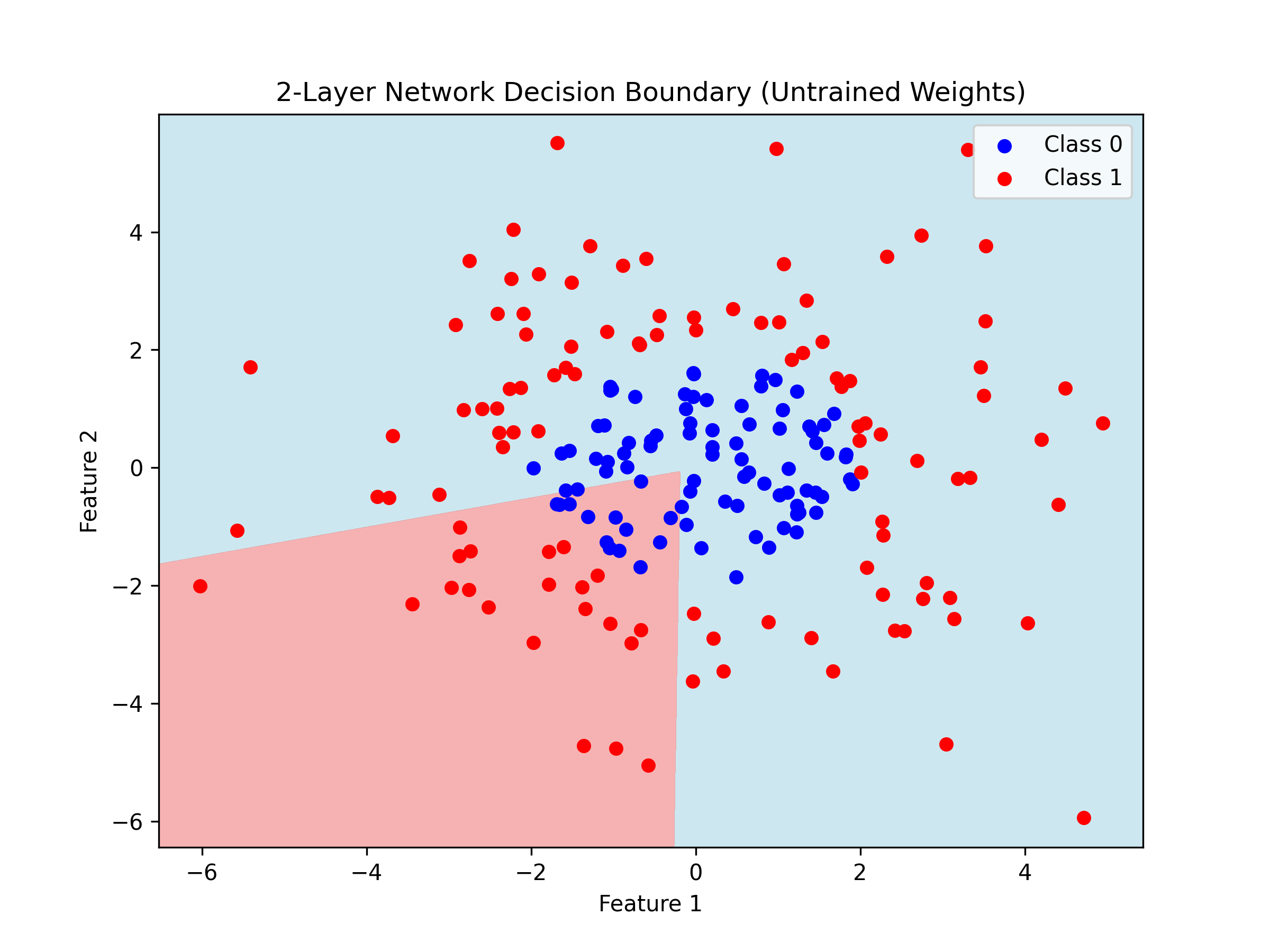
Starting from $\mathbf{a}^{(0)} = \mathbf{x}$ (the input), we compute forward through all layers to get the final output $\mathbf{a}^{(L)}$. Why does depth matter? Each layer learns a representation of the input at a different level of abstraction. Early layers (close to the input) learn low-level features: edges, corners, textures. Middle layers compose these into mid-level features: shapes, patterns. Deep layers recognise high-level semantic concepts: objects, entities, relationships. This hierarchy of representations is what makes deep networks powerful. A shallow network may need exponentially many neurons to capture such abstractions; a deeper network can build them up incrementally, using far fewer parameters.
The Universal Approximation Theorem states (roughly) that a feedforward network with one hidden layer and a nonlinear activation can approximate any continuous function on a compact domain, given enough hidden neurons. This is a powerful existence result: it guarantees that neural networks are expressive enough, in principle, to learn any relationship in the data. However, the theorem says nothing about how many neurons are needed (it could be astronomically large), how long training takes, or whether your optimisation algorithm will find a good solution. In practice, deeper networks with fewer total parameters often train faster and generalise better than shallow wide networks on real-world data.
::: {.callout-note icon="false"}
## 📘 Theory: Feedforward Forward Pass
:::
::: {.callout-tip icon="false"}
## 🔑 Key Formula
For a feedforward network with $L$ layers:
$$\mathbf{a}^{(\ell)} = f^{(\ell)}\left(\mathbf{W}^{(\ell)} \mathbf{a}^{(\ell-1)} + \mathbf{b}^{(\ell)}\right), \quad \ell = 1, 2, \ldots, L$$
with $\mathbf{a}^{(0)} = \mathbf{x}$ and output $\hat{\mathbf{y}} = \mathbf{a}^{(L)}$.
:::
::: {.panel-tabset}
## R
```{r}
#| label: feedforward-from-scratch
# Build a simple 2-layer feedforward network from scratch in R
# We'll use a synthetic dataset with 2 inputs, 1 output (binary classification)
set.seed(2974)
# Activation functions
sigmoid <- function(z) 1 / (1 + exp(-z))
relu <- function(z) { r <- pmax(0, z); dim(r) <- dim(z); r }
softmax <- function(z) {
exp_z <- exp(z - max(z))
exp_z / sum(exp_z)
}
# Feedforward pass for a 2-layer network
feedforward <- function(X, W1, b1, W2, b2) {
# Layer 1: hidden layer with ReLU
Z1 <- X %*% W1 + matrix(rep(b1, nrow(X)), nrow = nrow(X), byrow = TRUE)
A1 <- relu(Z1)
# Layer 2: output layer with sigmoid (binary classification)
Z2 <- A1 %*% W2 + matrix(rep(b2, nrow(X)), nrow = nrow(X), byrow = TRUE)
A2 <- sigmoid(Z2)
list(Z1 = Z1, A1 = A1, Z2 = Z2, A2 = A2)
}
# Generate synthetic data
n_samples <- 200
n_features <- 2
X <- matrix(rnorm(n_samples * n_features, sd = 2), nrow = n_samples, ncol = n_features)
# Nonlinear decision boundary: y = 1 if x1^2 + x2^2 > 4
Y <- as.numeric((X[, 1]^2 + X[, 2]^2) > 4)
# Initialize weights (small random values to break symmetry)
n_hidden <- 5
W1 <- matrix(rnorm(n_features * n_hidden, sd = 0.5), nrow = n_features, ncol = n_hidden)
b1 <- rnorm(n_hidden, sd = 0.1)
W2 <- matrix(rnorm(n_hidden * 1, sd = 0.5), nrow = n_hidden, ncol = 1)
b2 <- rnorm(1, sd = 0.1)
# Forward pass on the first 5 samples to show the computation
sample_indices <- 1:5
X_sample <- X[sample_indices, ]
results <- feedforward(X_sample, W1, b1, W2, b2)
cat("Sample inputs (first 5):\n")
print(X_sample)
cat("\nHidden layer activations (ReLU output):\n")
print(results$A1)
cat("\nNetwork output (sigmoid):\n")
print(results$A2)
cat("\nTrue labels:\n")
print(Y[sample_indices])
# Visualize the network architecture
cat("\n=== Network Architecture ===\n")
cat("Input layer: 2 neurons\n")
cat("Hidden layer: 5 neurons (ReLU)\n")
cat("Output layer: 1 neuron (Sigmoid)\n")
cat("Total parameters:", nrow(W1)*ncol(W1) + length(b1) + nrow(W2)*ncol(W2) + length(b2), "\n")
```
## Python
```{python}
#| label: py-feedforward-from-scratch
import numpy as np
import matplotlib.pyplot as plt
np.random.seed(2974)
# Activation functions
def sigmoid(z):
return 1 / (1 + np.exp(-z))
def relu(z):
return np.maximum(0, z)
# Feedforward pass for a 2-layer network
def feedforward(X, W1, b1, W2, b2):
# Layer 1: hidden layer with ReLU
Z1 = X @ W1 + b1
A1 = relu(Z1)
# Layer 2: output layer with sigmoid
Z2 = A1 @ W2 + b2
A2 = sigmoid(Z2)
return {"Z1": Z1, "A1": A1, "Z2": Z2, "A2": A2}
# Generate synthetic nonlinear data
n_samples = 200
n_features = 2
X = np.random.randn(n_samples, n_features) * 2
Y = ((X[:, 0]**2 + X[:, 1]**2) > 4).astype(int)
# Initialize weights
n_hidden = 5
W1 = np.random.randn(n_features, n_hidden) * 0.5
b1 = np.random.randn(n_hidden) * 0.1
W2 = np.random.randn(n_hidden, 1) * 0.5
b2 = np.random.randn(1) * 0.1
# Forward pass on sample
results = feedforward(X[:5], W1, b1, W2, b2)
print("Sample inputs (first 5):")
print(X[:5])
print("\nHidden layer activations (ReLU output):")
print(results['A1'])
print("\nNetwork output (sigmoid):")
print(results['A2'])
print("\nTrue labels:")
print(Y[:5])
# Visualize decision boundary
h = 0.02
x_min, x_max = X[:, 0].min() - 0.5, X[:, 0].max() + 0.5
y_min, y_max = X[:, 1].min() - 0.5, X[:, 1].max() + 0.5
xx, yy = np.meshgrid(np.arange(x_min, x_max, h),
np.arange(y_min, y_max, h))
Z_grid = np.c_[xx.ravel(), yy.ravel()]
predictions = feedforward(Z_grid, W1, b1, W2, b2)['A2'].reshape(xx.shape)
fig, ax = plt.subplots(figsize=(8, 6))
ax.contourf(xx, yy, predictions, levels=[0, 0.5, 1], colors=['lightblue', 'lightcoral'], alpha=0.6)
ax.scatter(X[Y == 0, 0], X[Y == 0, 1], c='blue', label='Class 0', s=30)
ax.scatter(X[Y == 1, 0], X[Y == 1, 1], c='red', label='Class 1', s=30)
ax.set_xlabel('Feature 1')
ax.set_ylabel('Feature 2')
ax.set_title('2-Layer Network Decision Boundary (Untrained Weights)')
ax.legend()
plt.show()
print("\n=== Network Architecture ===")
print(f"Input layer: {n_features} neurons")
print(f"Hidden layer: {n_hidden} neurons (ReLU)")
print(f"Output layer: 1 neuron (Sigmoid)")
print(f"Total parameters: {W1.size + b1.size + W2.size + b2.size}")
```
:::
::: {.callout-caution icon="false"}
## 📝 Section 33.3 Review Questions
1. What is the purpose of the hidden layer in a feedforward network? Why can't a single-layer network with the same total number of neurons fit a nonlinear boundary?
2. If a network has 5 input neurons, 10 hidden neurons (layer 1), 8 hidden neurons (layer 2), and 3 output neurons, how many weight matrices do we have? What are their dimensions?
3. The Universal Approximation Theorem guarantees that a single hidden layer can approximate any continuous function. Why do we still use deep networks in practice?
:::
## Loss Functions
A loss function quantifies how wrong the network's predictions are. During training, we adjust weights to minimise the loss. The choice of loss function depends on the task.
For regression (predicting a continuous value), Mean Squared Error (MSE) is standard:
$$L_{\text{MSE}} = \frac{1}{n} \sum_{i=1}^{n} (y_i - \hat{y}_i)^2$$
For binary classification, Binary Cross-Entropy (BCE) is nearly universal:
$$L_{\text{BCE}} = -\frac{1}{n} \sum_{i=1}^{n} \left[ y_i \log(\hat{y}_i) + (1 - y_i) \log(1 - \hat{y}_i) \right]$$
For multi-class classification (predicting one of $K$ classes), Categorical Cross-Entropy is used:
$$L_{\text{CCE}} = -\frac{1}{n} \sum_{i=1}^{n} \sum_{k=1}^{K} y_{i,k} \log(\hat{y}_{i,k})$$
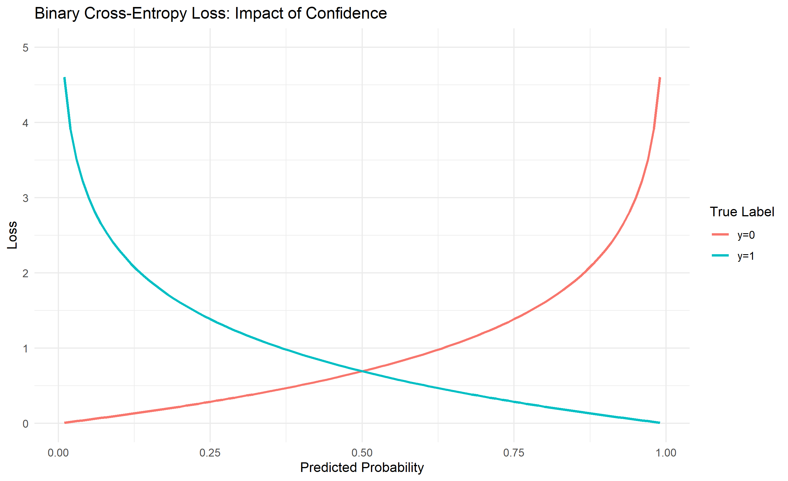
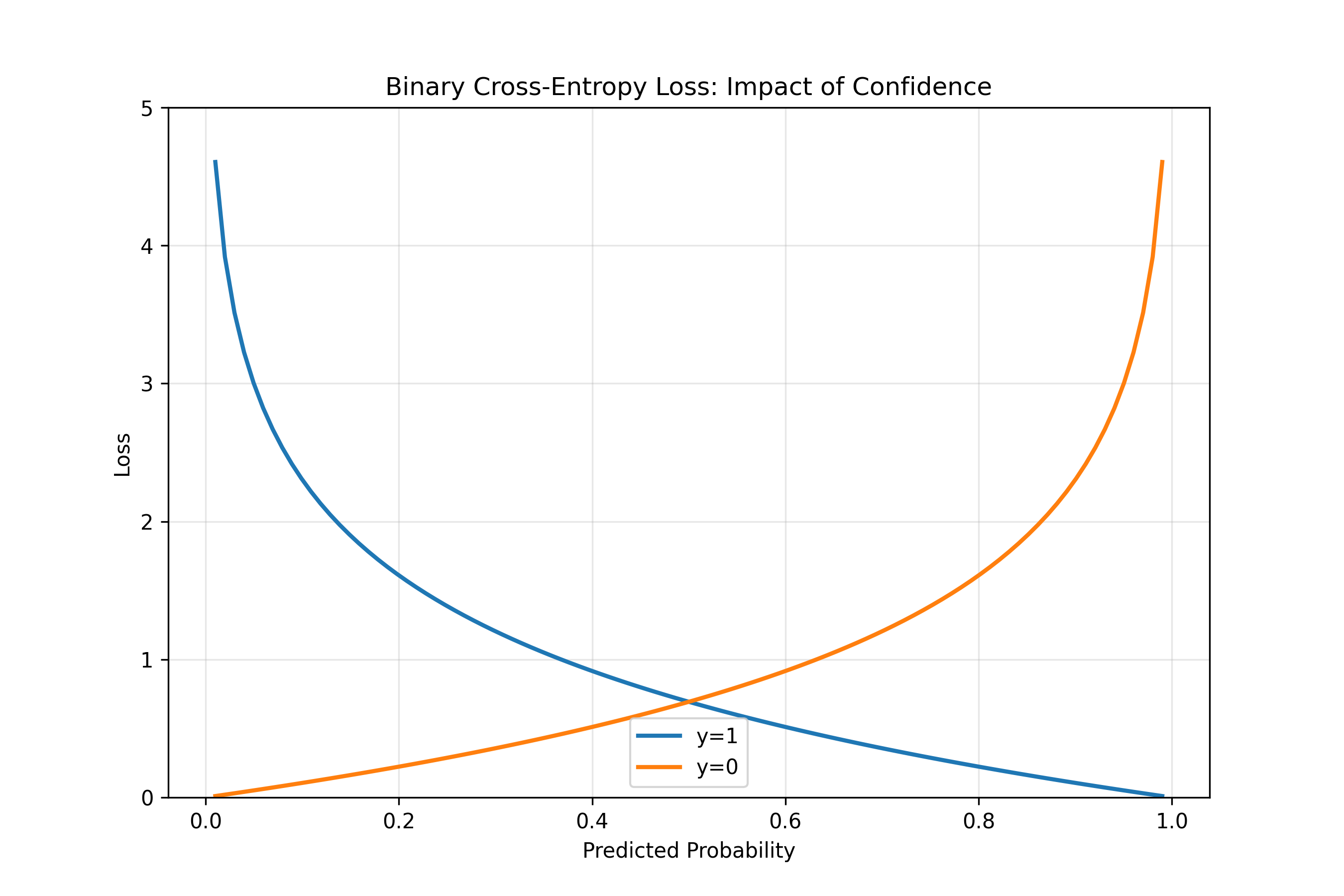
where $y_{i,k}$ is 1 if sample $i$ belongs to class $k$ and 0 otherwise, and $\hat{y}_{i,k}$ is the model's predicted probability for class $k$. Cross-entropy penalises confident wrong predictions heavily. If the true label is $y = 1$ but the model predicts $\hat{y} = 0.99$, the loss is small. If $\hat{y} = 0.01$, the loss is large (approximately $-\log(0.01) \approx 4.6$). This makes sense: being confidently wrong is worse than being uncertainly right.
::: {.callout-note icon="false"}
## 📘 Theory: Loss Functions for Machine Learning Tasks
:::
::: {.callout-tip icon="false"}
## 🔑 Key Formula
**Mean Squared Error (Regression):**
$$L = \frac{1}{n} \sum_{i=1}^{n} (y_i - \hat{y}_i)^2$$
**Binary Cross-Entropy (Binary Classification):**
$$L = -\frac{1}{n} \sum_{i=1}^{n} \left[ y_i \log(\hat{y}_i) + (1-y_i) \log(1-\hat{y}_i) \right]$$
**Categorical Cross-Entropy (Multi-class):**
$$L = -\frac{1}{n} \sum_{i=1}^{n} \sum_{k=1}^{K} y_{i,k} \log(\hat{y}_{i,k})$$
:::
::: {.panel-tabset}
## R
```{r}
#| label: loss-functions
# Compute loss functions
binary_cross_entropy <- function(y_true, y_pred) {
# Clip predictions to avoid log(0)
y_pred <- pmax(pmin(y_pred, 1 - 1e-7), 1e-7)
loss <- -mean(y_true * log(y_pred) + (1 - y_true) * log(1 - y_pred))
return(loss)
}
mean_squared_error <- function(y_true, y_pred) {
loss <- mean((y_true - y_pred)^2)
return(loss)
}
categorical_cross_entropy <- function(y_true_matrix, y_pred_probs) {
# y_true_matrix: n x K one-hot encoded matrix
# y_pred_probs: n x K prediction probability matrix
y_pred_probs <- pmax(pmin(y_pred_probs, 1 - 1e-7), 1e-7)
loss <- -mean(rowSums(y_true_matrix * log(y_pred_probs)))
return(loss)
}
# Example: Binary classification
set.seed(5183)
y_true_binary <- c(0, 1, 1, 0, 1)
y_pred_binary <- c(0.1, 0.8, 0.9, 0.3, 0.6)
bce_loss <- binary_cross_entropy(y_true_binary, y_pred_binary)
cat("Binary Cross-Entropy Loss:", round(bce_loss, 4), "\n")
# Example: Regression
y_true_reg <- c(1.0, 2.5, 3.2, 0.8, 4.1)
y_pred_reg <- c(1.1, 2.3, 3.5, 0.5, 4.2)
mse_loss <- mean_squared_error(y_true_reg, y_pred_reg)
cat("Mean Squared Error Loss:", round(mse_loss, 4), "\n")
# Example: Multi-class classification (3 classes)
y_true_multiclass <- matrix(c(
1, 0, 0,
0, 1, 0,
0, 0, 1,
1, 0, 0,
0, 1, 0
), nrow = 5, ncol = 3, byrow = TRUE)
y_pred_multiclass <- matrix(c(
0.7, 0.2, 0.1,
0.1, 0.8, 0.1,
0.1, 0.2, 0.7,
0.6, 0.3, 0.1,
0.2, 0.7, 0.1
), nrow = 5, ncol = 3, byrow = TRUE)
cce_loss <- categorical_cross_entropy(y_true_multiclass, y_pred_multiclass)
cat("Categorical Cross-Entropy Loss:", round(cce_loss, 4), "\n")
# Visualize the effect of prediction confidence on BCE loss
pred_range <- seq(0.01, 0.99, by = 0.01)
loss_y_true_1 <- -log(pred_range) # Loss when true label is 1
loss_y_true_0 <- -log(1 - pred_range) # Loss when true label is 0
df_loss <- data.frame(
prediction = c(pred_range, pred_range),
loss = c(loss_y_true_1, loss_y_true_0),
true_label = c(rep("y=1", length(pred_range)), rep("y=0", length(pred_range)))
)
library(ggplot2)
ggplot(df_loss, aes(x = prediction, y = loss, colour = true_label)) +
geom_line(linewidth = 1) +
theme_minimal() +
labs(
title = "Binary Cross-Entropy Loss: Impact of Confidence",
x = "Predicted Probability",
y = "Loss",
colour = "True Label"
) +
ylim(0, 5)
```
## Python
```{python}
#| label: py-loss-functions
import numpy as np
import matplotlib.pyplot as plt
def binary_cross_entropy(y_true, y_pred):
# Clip predictions to avoid log(0)
y_pred = np.clip(y_pred, 1e-7, 1 - 1e-7)
loss = -np.mean(y_true * np.log(y_pred) + (1 - y_true) * np.log(1 - y_pred))
return loss
def mean_squared_error(y_true, y_pred):
loss = np.mean((y_true - y_pred)**2)
return loss
def categorical_cross_entropy(y_true, y_pred):
# y_true: one-hot encoded (n x K)
# y_pred: predicted probabilities (n x K)
y_pred = np.clip(y_pred, 1e-7, 1 - 1e-7)
loss = -np.mean(np.sum(y_true * np.log(y_pred), axis=1))
return loss
# Example: Binary classification
y_true_binary = np.array([0, 1, 1, 0, 1])
y_pred_binary = np.array([0.1, 0.8, 0.9, 0.3, 0.6])
bce = binary_cross_entropy(y_true_binary, y_pred_binary)
print(f"Binary Cross-Entropy Loss: {bce:.4f}")
# Example: Regression
y_true_reg = np.array([1.0, 2.5, 3.2, 0.8, 4.1])
y_pred_reg = np.array([1.1, 2.3, 3.5, 0.5, 4.2])
mse = mean_squared_error(y_true_reg, y_pred_reg)
print(f"Mean Squared Error Loss: {mse:.4f}")
# Example: Multi-class classification
y_true_multiclass = np.array([
[1, 0, 0],
[0, 1, 0],
[0, 0, 1],
[1, 0, 0],
[0, 1, 0]
])
y_pred_multiclass = np.array([
[0.7, 0.2, 0.1],
[0.1, 0.8, 0.1],
[0.1, 0.2, 0.7],
[0.6, 0.3, 0.1],
[0.2, 0.7, 0.1]
])
cce = categorical_cross_entropy(y_true_multiclass, y_pred_multiclass)
print(f"Categorical Cross-Entropy Loss: {cce:.4f}")
# Visualize BCE loss
pred_range = np.linspace(0.01, 0.99, 100)
loss_y_true_1 = -np.log(pred_range)
loss_y_true_0 = -np.log(1 - pred_range)
fig, ax = plt.subplots(figsize=(9, 6))
ax.plot(pred_range, loss_y_true_1, label='y=1', linewidth=2)
ax.plot(pred_range, loss_y_true_0, label='y=0', linewidth=2)
ax.set_xlabel('Predicted Probability')
ax.set_ylabel('Loss')
ax.set_title('Binary Cross-Entropy Loss: Impact of Confidence')
ax.legend()
ax.set_ylim(0, 5)
ax.grid(True, alpha=0.3)
plt.show()
print("\nNote: BCE loss is 0 only when prediction matches reality perfectly,")
print("and increases sharply as confidence in wrong prediction increases.")
```
:::
::: {.callout-caution icon="false"}
## 📝 Section 33.4 Review Questions
1. Why does cross-entropy loss penalise confident wrong predictions more heavily than MSE?
2. If a binary classification model predicts $\hat{y} = 0.99$ for a sample with true label $y = 0$, compute the BCE loss contribution.
3. In multi-class classification, why do we use one-hot encoding for the true labels when computing categorical cross-entropy?
:::
## Backpropagation
Backpropagation is the algorithm for computing gradients of the loss with respect to every weight in the network. It exploits the chain rule of calculus to do this efficiently. The key insight is elegant: compute the gradient of the loss with respect to the output, then flow that gradient backward through each layer, accumulating the effect of each layer's weights on the loss.
Consider a simple case: a 2-layer network with loss $L$. We want $\frac{\partial L}{\partial w_{ij}}$ for every weight $w_{ij}$. By the chain rule,
$$\frac{\partial L}{\partial w_{ij}^{(2)}} = \frac{\partial L}{\partial \hat{y}} \cdot \frac{\partial \hat{y}}{\partial z_i^{(2)}} \cdot \frac{\partial z_i^{(2)}}{\partial w_{ij}^{(2)}}$$
Define $\delta_i^{(2)} = \frac{\partial L}{\partial z_i^{(2)}}$ (the "error" at layer 2). Then $\frac{\partial L}{\partial w_{ij}^{(2)}} = \delta_i^{(2)} \cdot a_j^{(1)}$. Now, to compute gradients with respect to weights in layer 1, we need $\delta^{(1)}$. By the chain rule:
$$\delta_j^{(1)} = \frac{\partial L}{\partial a_j^{(1)}} \cdot \frac{\partial a_j^{(1)}}{\partial z_j^{(1)}} = \left(\sum_i \delta_i^{(2)} w_{ij}^{(2)}\right) \cdot f'(z_j^{(1)})$$
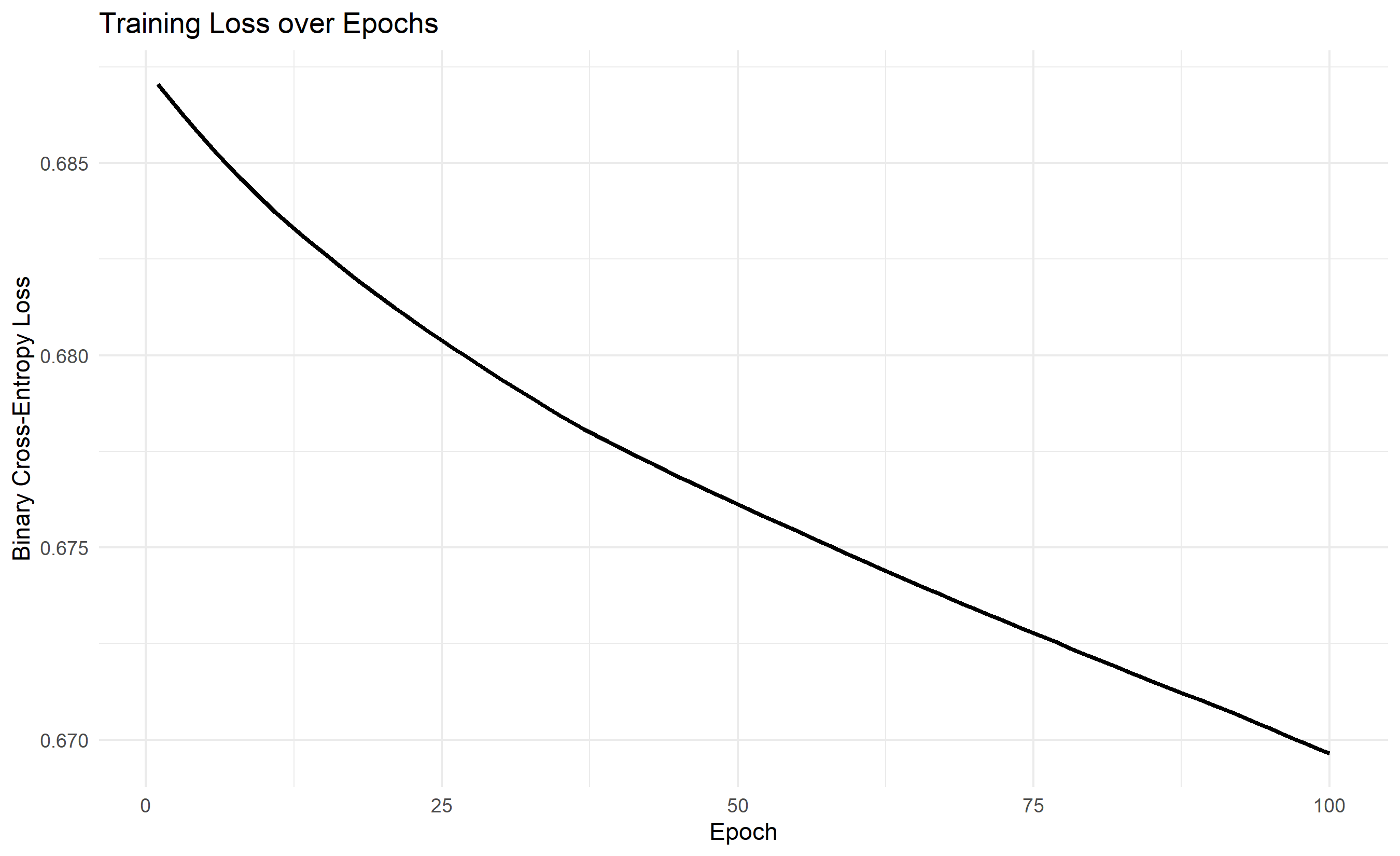
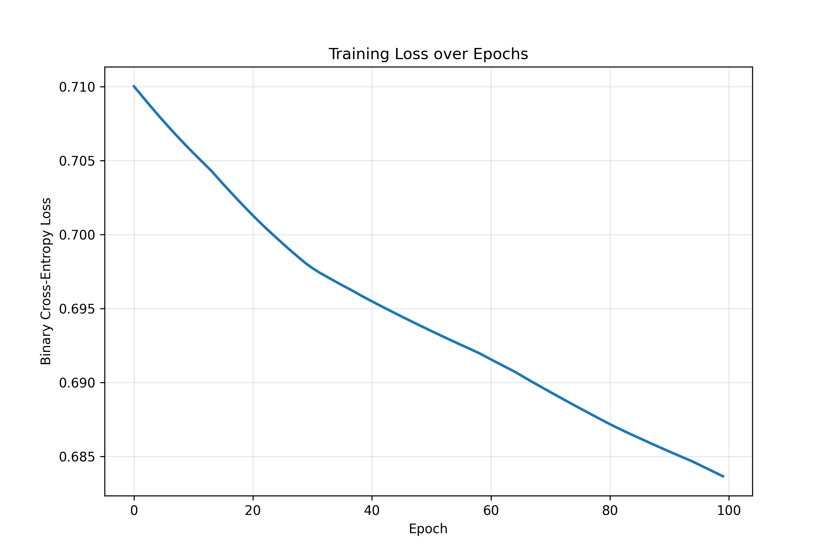
So we can compute $\delta^{(1)}$ from $\delta^{(2)}$ by multiplying by the weight matrix transpose and the derivative of the activation function. This is the "backpropagation" step: the error flows backward through the network, getting transformed by each layer's weights and activations. For deep networks, this means the gradient of an early layer's weight is the product of many terms: a loss derivative, several activation derivatives, and several weight matrices. If each activation derivative is less than 1 (as with sigmoid), these products shrink exponentially with depth—the vanishing gradient problem. ReLU mitigates this because its derivative is exactly 1 for positive inputs and 0 for negative inputs, so the product doesn't shrink as aggressively.
::: {.callout-note icon="false"}
## 📘 Theory: Chain Rule and Backpropagation
:::
::: {.callout-tip icon="false"}
## 🔑 Key Formula
For a loss $L$ and weights through layers, the gradient flows backward via the chain rule:
$$\frac{\partial L}{\partial w^{(\ell)}} = \frac{\partial L}{\partial z^{(\ell)}} \cdot \frac{\partial z^{(\ell)}}{\partial w^{(\ell)}}$$
Define the error term $\delta^{(\ell)} = \frac{\partial L}{\partial z^{(\ell)}}$. Then:
$$\delta^{(\ell)} = \left(\delta^{(\ell+1)^T} \mathbf{W}^{(\ell+1)}\right) \odot f'(\mathbf{z}^{(\ell)})$$
where $\odot$ denotes element-wise multiplication (Hadamard product).
:::
::: {.panel-tabset}
## R
```{r}
#| label: backpropagation-simple
# Implement backpropagation for a simple 2-layer network
set.seed(8416)
# Activation functions and their derivatives
sigmoid <- function(z) 1 / (1 + exp(-z))
sigmoid_deriv <- function(a) a * (1 - a) # a is the activation, not z
relu <- function(z) { r <- pmax(0, z); dim(r) <- dim(z); r }
relu_deriv <- function(z) as.numeric(z > 0)
# Binary cross-entropy loss
bce_loss <- function(y, y_pred) {
y_pred <- pmax(pmin(y_pred, 1 - 1e-7), 1e-7)
-mean(y * log(y_pred) + (1 - y) * log(1 - y_pred))
}
# Compute gradients via backpropagation
backpropagate <- function(X, y, W1, b1, W2, b2) {
n <- nrow(X)
# Forward pass
Z1 <- X %*% W1 + matrix(rep(b1, n), nrow = n, byrow = TRUE)
A1 <- relu(Z1)
Z2 <- A1 %*% W2 + matrix(rep(b2, n), nrow = n, byrow = TRUE)
A2 <- sigmoid(Z2)
# Backward pass: compute loss and gradients
loss <- bce_loss(y, A2)
# Output layer error
dZ2 <- (A2 - y) / n # Derivative of BCE with sigmoid output
dW2 <- t(A1) %*% dZ2
db2 <- colMeans(dZ2)
# Hidden layer error
dA1 <- dZ2 %*% t(W2)
dZ1 <- dA1 * relu_deriv(Z1)
dW1 <- t(X) %*% dZ1
db1 <- colMeans(dZ1)
list(
loss = loss,
dW1 = dW1, db1 = db1,
dW2 = dW2, db2 = db2,
A1 = A1, A2 = A2, Z1 = Z1, Z2 = Z2
)
}
# Generate synthetic data
n_samples <- 100
X <- matrix(rnorm(n_samples * 2), nrow = n_samples, ncol = 2)
y <- as.numeric((X[, 1]^2 + X[, 2]^2) > 2)
y <- matrix(y, ncol = 1)
# Initialize weights
W1 <- matrix(rnorm(2 * 5, sd = 0.5), nrow = 2, ncol = 5)
b1 <- rnorm(5, sd = 0.1)
W2 <- matrix(rnorm(5 * 1, sd = 0.5), nrow = 5, ncol = 1)
b2 <- rnorm(1, sd = 0.1)
# Training loop
learning_rate <- 0.1
n_epochs <- 100
loss_history <- numeric(n_epochs)
for (epoch in 1:n_epochs) {
grads <- backpropagate(X, y, W1, b1, W2, b2)
loss_history[epoch] <- grads$loss
# Update weights with gradient descent
W2 <- W2 - learning_rate * grads$dW2
b2 <- b2 - learning_rate * grads$db2
W1 <- W1 - learning_rate * grads$dW1
b1 <- b1 - learning_rate * grads$db1
if (epoch %% 20 == 0) {
cat("Epoch", epoch, "Loss:", round(grads$loss, 4), "\n")
}
}
# Plot loss history
library(ggplot2)
df_loss <- data.frame(epoch = 1:n_epochs, loss = loss_history)
ggplot(df_loss, aes(x = epoch, y = loss)) +
geom_line(linewidth = 1) +
theme_minimal() +
labs(
title = "Training Loss over Epochs",
x = "Epoch",
y = "Binary Cross-Entropy Loss"
)
```
## Python
```{python}
#| label: py-backpropagation-simple
import numpy as np
import matplotlib.pyplot as plt
np.random.seed(8416)
# Activation functions and derivatives
def sigmoid(z):
return 1 / (1 + np.exp(-z))
def sigmoid_deriv(a):
return a * (1 - a)
def relu(z):
return np.maximum(0, z)
def relu_deriv(z):
return (z > 0).astype(float)
# Binary cross-entropy loss
def bce_loss(y, y_pred):
y_pred = np.clip(y_pred, 1e-7, 1 - 1e-7)
return -np.mean(y * np.log(y_pred) + (1 - y) * np.log(1 - y_pred))
# Backpropagation
def backpropagate(X, y, W1, b1, W2, b2):
n = X.shape[0]
# Forward pass
Z1 = X @ W1 + b1
A1 = relu(Z1)
Z2 = A1 @ W2 + b2
A2 = sigmoid(Z2)
# Backward pass
loss = bce_loss(y, A2)
# Output layer error
dZ2 = (A2 - y) / n
dW2 = A1.T @ dZ2
db2 = np.mean(dZ2, axis=0, keepdims=True)
# Hidden layer error
dA1 = dZ2 @ W2.T
dZ1 = dA1 * relu_deriv(Z1)
dW1 = X.T @ dZ1
db1 = np.mean(dZ1, axis=0)
return {
'loss': loss,
'dW1': dW1, 'db1': db1,
'dW2': dW2, 'db2': db2,
'A1': A1, 'A2': A2, 'Z1': Z1, 'Z2': Z2
}
# Generate synthetic data
n_samples = 100
X = np.random.randn(n_samples, 2)
y = ((X[:, 0]**2 + X[:, 1]**2) > 2).astype(int).reshape(-1, 1)
# Initialize weights
W1 = np.random.randn(2, 5) * 0.5
b1 = np.random.randn(1, 5) * 0.1
W2 = np.random.randn(5, 1) * 0.5
b2 = np.random.randn(1, 1) * 0.1
# Training loop
learning_rate = 0.1
n_epochs = 100
loss_history = []
for epoch in range(n_epochs):
grads = backpropagate(X, y, W1, b1, W2, b2)
loss_history.append(grads['loss'])
# Update weights
W2 -= learning_rate * grads['dW2']
b2 -= learning_rate * grads['db2']
W1 -= learning_rate * grads['dW1']
b1 -= learning_rate * grads['db1']
if (epoch + 1) % 20 == 0:
print(f"Epoch {epoch + 1} Loss: {grads['loss']:.4f}")
# Plot loss history
plt.figure(figsize=(9, 6))
plt.plot(loss_history, linewidth=2)
plt.xlabel('Epoch')
plt.ylabel('Binary Cross-Entropy Loss')
plt.title('Training Loss over Epochs')
plt.grid(True, alpha=0.3)
plt.show()
# Final predictions
Z1 = X @ W1 + b1
A1 = relu(Z1)
Z2 = A1 @ W2 + b2
A2 = sigmoid(Z2)
accuracy = np.mean((A2 > 0.5).astype(int) == y)
print(f"\nFinal accuracy: {accuracy:.4f}")
```
:::
::: {.callout-caution icon="false"}
## 📝 Section 33.5 Review Questions
1. Explain in plain English why the gradient computed via backpropagation is correct (hint: what does the chain rule say?).
2. If a network has 4 layers and you want the gradient $\frac{\partial L}{\partial w^{(1)}}$, how many weight matrices must appear in this product of derivatives?
3. Why does ReLU's derivative being exactly 1 for positive inputs help alleviate vanishing gradients compared to sigmoid?
:::
## Gradient Descent and Optimisers
Once we have gradients via backpropagation, we need to update weights. Gradient descent is the most basic approach: move each weight in the opposite direction of its gradient, scaled by a learning rate $\alpha$:
$$w := w - \alpha \frac{\partial L}{\partial w}$$
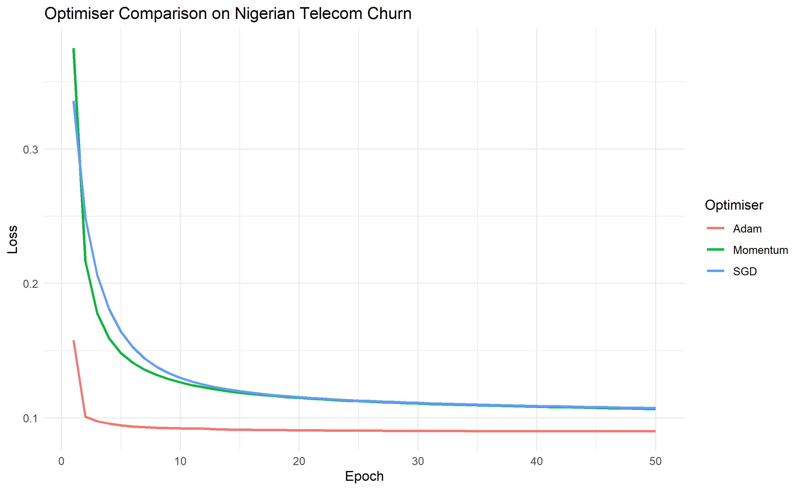
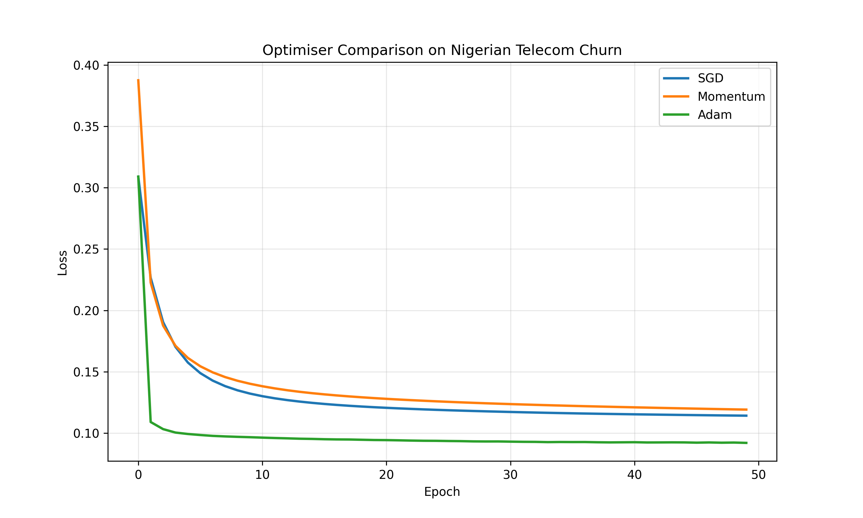
There are three variants. Batch gradient descent computes the loss and gradient on the entire training set before updating weights—this is accurate but slow on large datasets. Stochastic gradient descent (SGD) updates after every single example—this is noisy but fast and can escape sharp minima. Mini-batch gradient descent (the modern standard) processes batches of, say, 32 or 128 examples at a time—it balances noise and efficiency. The learning rate is crucial: too large and the loss diverges; too small and training crawls. Setting it requires trial and error or adaptive schemes.
Momentum addresses a problem with vanilla gradient descent: oscillation. If the gradient changes sign (as in a ravine), the loss bounces around. Momentum accumulates past gradients: $v := \beta v + (1 - \beta) \nabla L$, then $w := w - \alpha v$. The parameter $\beta$ (typically 0.9) acts as a memory: recent gradients have more weight. This smooths out oscillations and accelerates convergence. The Adam optimiser (Adaptive Moment Estimation) goes further: it maintains both a momentum term (first moment) and a term proportional to the squared gradient (second moment), and adapts the learning rate for each parameter independently. In practice, Adam is often the default choice because it requires less hyperparameter tuning.
Weight initialisation matters more than it appears. If all weights start at zero, all hidden units will be identical (they receive identical inputs, compute identical values, and receive identical gradients—no learning occurs). If weights are too large, activations explode or saturate. Xavier initialisation initialises weights by sampling from a distribution with variance $\frac{1}{n_{\text{in}}}$, where $n_{\text{in}}$ is the number of inputs to a neuron. He initialisation, used with ReLU, samples with variance $\frac{2}{n_{\text{in}}}$. Both ensure activations have reasonable magnitude.
::: {.callout-note icon="false"}
## 📘 Theory: Optimisation Algorithms
:::
::: {.callout-tip icon="false"}
## 🔑 Key Formula
**Momentum:**
$$v_t = \beta v_{t-1} + (1-\beta) \nabla L, \quad w_t = w_{t-1} - \alpha v_t$$
**Adam (Adaptive Moment Estimation):**
$$m_t = \beta_1 m_{t-1} + (1-\beta_1) \nabla L$$
$$s_t = \beta_2 s_{t-1} + (1-\beta_2) (\nabla L)^2$$
$$w_t = w_{t-1} - \alpha \frac{m_t}{\sqrt{s_t} + \epsilon}$$
(Typical: $\beta_1 = 0.9$, $\beta_2 = 0.999$, $\epsilon = 10^{-8}$)
:::
::: {.panel-tabset}
## R
```{r}
#| label: optimisers-comparison
# Compare different optimisers on a real dataset: Nigerian telecom churn

library(ggplot2)
library(dplyr)

set.seed(3752)

# Generate synthetic Nigerian telecom churn dataset
n_customers <- 5000
tenure <- runif(n_customers, 1, 72)
arpu <- rnorm(n_customers, mean = 5000, sd = 2000)  # Nigerian Naira
data_usage <- rnorm(n_customers, mean = 500, sd = 200)  # MB per month
voice_minutes <- rnorm(n_customers, mean = 800, sd = 400)
recharge_freq <- runif(n_customers, 1, 30)  # days between recharges
network_issues <- rpois(n_customers, lambda = 2)

# Churn probability depends on multiple factors
churn_prob <- 0.1 + 0.001 * (1 / (tenure + 1)) - 0.00001 * arpu - 0.0001 * data_usage + 0.01 * network_issues
churn_prob <- pmax(pmin(churn_prob, 1), 0)
churn <- as.numeric(runif(n_customers) < churn_prob)

# Prepare data
X <- cbind(
  tenure = scale(tenure)[, 1],
  arpu = scale(arpu)[, 1],
  data_usage = scale(data_usage)[, 1],
  voice_minutes = scale(voice_minutes)[, 1],
  recharge_freq = scale(recharge_freq)[, 1],
  network_issues = scale(network_issues)[, 1]
)
y <- matrix(churn, ncol = 1)

# Neural network training function with different optimisers
train_network <- function(X, y, optimiser = "sgd", epochs = 50) {
  n <- nrow(X)
  n_features <- ncol(X)
  n_hidden <- 10
  batch_size <- 32
  learning_rate <- 0.01

  # Initialize
  W1 <- matrix(rnorm(n_features * n_hidden, sd = sqrt(2 / n_features)), nrow = n_features, ncol = n_hidden)
  b1 <- rnorm(n_hidden, sd = 0.01)
  W2 <- matrix(rnorm(n_hidden * 1, sd = sqrt(2 / n_hidden)), nrow = n_hidden, ncol = 1)
  b2 <- rnorm(1, sd = 0.01)

  # Optimizer state
  if (optimiser == "momentum") {
    vW1 <- matrix(0, nrow = nrow(W1), ncol = ncol(W1))
    vb1 <- rep(0, length(b1))
    vW2 <- matrix(0, nrow = nrow(W2), ncol = ncol(W2))
    vb2 <- rep(0, length(b2))
    beta <- 0.9
  } else if (optimiser == "adam") {
    mW1 <- matrix(0, nrow = nrow(W1), ncol = ncol(W1))
    vW1 <- matrix(0, nrow = nrow(W1), ncol = ncol(W1))
    mb1 <- rep(0, length(b1))
    vb1 <- rep(0, length(b1))
    mW2 <- matrix(0, nrow = nrow(W2), ncol = ncol(W2))
    vW2 <- matrix(0, nrow = nrow(W2), ncol = ncol(W2))
    mb2 <- rep(0, length(b2))
    vb2 <- rep(0, length(b2))
    beta1 <- 0.9
    beta2 <- 0.999
    epsilon <- 1e-8
    t <- 0
  }

  loss_history <- numeric(epochs)

  for (epoch in 1:epochs) {
    epoch_loss <- 0
    n_batches <- ceiling(n / batch_size)

    for (batch in 1:n_batches) {
      idx <- ((batch - 1) * batch_size + 1):min(batch * batch_size, n)
      X_batch <- X[idx, , drop = FALSE]
      y_batch <- y[idx, , drop = FALSE]

      # Forward pass
      Z1 <- X_batch %*% W1 + matrix(rep(b1, nrow(X_batch)), nrow = nrow(X_batch), byrow = TRUE)
      { A1 <- pmax(0, Z1); dim(A1) <- dim(Z1) }  # ReLU, preserving matrix shape
      Z2 <- A1 %*% W2 + matrix(rep(b2, nrow(X_batch)), nrow = nrow(X_batch), byrow = TRUE)
      A2 <- 1 / (1 + exp(-Z2))  # Sigmoid

      # Loss
      A2_clipped <- pmax(pmin(A2, 1 - 1e-7), 1e-7)
      batch_loss <- -mean(y_batch * log(A2_clipped) + (1 - y_batch) * log(1 - A2_clipped))
      epoch_loss <- epoch_loss + batch_loss

      # Backward pass
      dZ2 <- (A2 - y_batch) / nrow(X_batch)
      dW2 <- t(A1) %*% dZ2
      db2 <- colMeans(dZ2)

      dA1 <- dZ2 %*% t(W2)
      dZ1 <- dA1 * (Z1 > 0)  # ReLU derivative
      dW1 <- t(X_batch) %*% dZ1
      db1 <- colMeans(dZ1)

      # Update based on optimiser
      if (optimiser == "sgd") {
        W2 <- W2 - learning_rate * dW2
        b2 <- b2 - learning_rate * db2
        W1 <- W1 - learning_rate * dW1
        b1 <- b1 - learning_rate * db1
      } else if (optimiser == "momentum") {
        vW2 <- beta * vW2 + (1 - beta) * dW2
        vb2 <- beta * vb2 + (1 - beta) * db2
        vW1 <- beta * vW1 + (1 - beta) * dW1
        vb1 <- beta * vb1 + (1 - beta) * db1

        W2 <- W2 - learning_rate * vW2
        b2 <- b2 - learning_rate * vb2
        W1 <- W1 - learning_rate * vW1
        b1 <- b1 - learning_rate * vb1
      } else if (optimiser == "adam") {
        t <- t + 1
        mW2 <- beta1 * mW2 + (1 - beta1) * dW2
        vW2 <- beta2 * vW2 + (1 - beta2) * (dW2^2)
        mb2 <- beta1 * mb2 + (1 - beta1) * db2
        vb2 <- beta2 * vb2 + (1 - beta2) * (db2^2)

        mW2_hat <- mW2 / (1 - beta1^t)
        vW2_hat <- vW2 / (1 - beta2^t)
        mb2_hat <- mb2 / (1 - beta1^t)
        vb2_hat <- vb2 / (1 - beta2^t)

        W2 <- W2 - learning_rate * mW2_hat / (sqrt(vW2_hat) + epsilon)
        b2 <- b2 - learning_rate * mb2_hat / (sqrt(vb2_hat) + epsilon)

        # Similar for layer 1
        mW1 <- beta1 * mW1 + (1 - beta1) * dW1
        vW1 <- beta2 * vW1 + (1 - beta2) * (dW1^2)
        mb1 <- beta1 * mb1 + (1 - beta1) * db1
        vb1 <- beta2 * vb1 + (1 - beta2) * (db1^2)

        mW1_hat <- mW1 / (1 - beta1^t)
        vW1_hat <- vW1 / (1 - beta2^t)
        mb1_hat <- mb1 / (1 - beta1^t)
        vb1_hat <- vb1 / (1 - beta2^t)

        W1 <- W1 - learning_rate * mW1_hat / (sqrt(vW1_hat) + epsilon)
        b1 <- b1 - learning_rate * mb1_hat / (sqrt(vb1_hat) + epsilon)
      }
    }

    loss_history[epoch] <- epoch_loss / n_batches
  }

  return(loss_history)
}

# Train with each optimiser
loss_sgd <- train_network(X, y, optimiser = "sgd", epochs = 50)
loss_momentum <- train_network(X, y, optimiser = "momentum", epochs = 50)
loss_adam <- train_network(X, y, optimiser = "adam", epochs = 50)

# Compare
df_comparison <- data.frame(
  epoch = rep(1:50, 3),
  loss = c(loss_sgd, loss_momentum, loss_adam),
  optimiser = rep(c("SGD", "Momentum", "Adam"), each = 50)
)

ggplot(df_comparison, aes(x = epoch, y = loss, colour = optimiser)) +
  geom_line(linewidth = 1) +
  theme_minimal() +
  labs(
    title = "Optimiser Comparison on Nigerian Telecom Churn",
    x = "Epoch",
    y = "Loss",
    colour = "Optimiser"
  )
```
## Python
```{python}
#| label: py-optimisers-comparison
import numpy as np
import matplotlib.pyplot as plt

np.random.seed(3752)

# Generate synthetic Nigerian telecom churn data
n_customers = 5000
tenure = np.random.uniform(1, 72, n_customers)
arpu = np.random.normal(5000, 2000, n_customers)
data_usage = np.random.normal(500, 200, n_customers)
voice_minutes = np.random.normal(800, 400, n_customers)
recharge_freq = np.random.uniform(1, 30, n_customers)
network_issues = np.random.poisson(2, n_customers)

# Churn probability
churn_prob = (0.1 + 0.001 / (tenure + 1) - 0.00001 * arpu -
              0.0001 * data_usage + 0.01 * network_issues)
churn_prob = np.clip(churn_prob, 0, 1)
churn = (np.random.rand(n_customers) < churn_prob).astype(int)

# Standardize features
X = np.column_stack([tenure, arpu, data_usage, voice_minutes, recharge_freq, network_issues])
X = (X - X.mean(axis=0)) / (X.std(axis=0) + 1e-8)
y = churn.reshape(-1, 1)

def train_network(X, y, optimiser='sgd', epochs=50):
    n, n_features = X.shape
    n_hidden = 10
    batch_size = 32
    learning_rate = 0.01

    # Initialize with He initialisation
    W1 = np.random.randn(n_features, n_hidden) * np.sqrt(2 / n_features)
    b1 = np.random.randn(1, n_hidden) * 0.01
    W2 = np.random.randn(n_hidden, 1) * np.sqrt(2 / n_hidden)
    b2 = np.random.randn(1, 1) * 0.01

    # Optimizer state
    if optimiser == 'momentum':
        vW1 = np.zeros_like(W1)
        vb1 = np.zeros_like(b1)
        vW2 = np.zeros_like(W2)
        vb2 = np.zeros_like(b2)
        beta = 0.9
    elif optimiser == 'adam':
        mW1 = np.zeros_like(W1)
        vW1 = np.zeros_like(W1)
        mb1 = np.zeros_like(b1)
        vb1 = np.zeros_like(b1)
        mW2 = np.zeros_like(W2)
        vW2 = np.zeros_like(W2)
        mb2 = np.zeros_like(b2)
        vb2 = np.zeros_like(b2)
        beta1, beta2, epsilon = 0.9, 0.999, 1e-8
        t = 0

    loss_history = []

    for epoch in range(epochs):
        epoch_loss = 0
        n_batches = int(np.ceil(n / batch_size))

        for batch in range(n_batches):
            idx = slice(batch * batch_size, min((batch + 1) * batch_size, n))
            X_batch = X[idx]
            y_batch = y[idx]

            # Forward
            Z1 = X_batch @ W1 + b1
            A1 = np.maximum(0, Z1)
            Z2 = A1 @ W2 + b2
            A2 = 1 / (1 + np.exp(-Z2))

            # Loss
            A2_clipped = np.clip(A2, 1e-7, 1 - 1e-7)
            batch_loss = -np.mean(y_batch * np.log(A2_clipped) +
                                (1 - y_batch) * np.log(1 - A2_clipped))
            epoch_loss += batch_loss

            # Backward
            dZ2 = (A2 - y_batch) / len(X_batch)
            dW2 = A1.T @ dZ2
            db2 = np.mean(dZ2, axis=0, keepdims=True)

            dA1 = dZ2 @ W2.T
            dZ1 = dA1 * (Z1 > 0)
            dW1 = X_batch.T @ dZ1
            db1 = np.mean(dZ1, axis=0, keepdims=True)

            # Update
            if optimiser == 'sgd':
                W2 -= learning_rate * dW2
                b2 -= learning_rate * db2
                W1 -= learning_rate * dW1
                b1 -= learning_rate * db1
            elif optimiser == 'momentum':
                vW2 = beta * vW2 + (1 - beta) * dW2
                vb2 = beta * vb2 + (1 - beta) * db2
                vW1 = beta * vW1 + (1 - beta) * dW1
                vb1 = beta * vb1 + (1 - beta) * db1

                W2 -= learning_rate * vW2
                b2 -= learning_rate * vb2
                W1 -= learning_rate * vW1
                b1 -= learning_rate * vb1
            elif optimiser == 'adam':
                t += 1
                mW2 = beta1 * mW2 + (1 - beta1) * dW2
                vW2 = beta2 * vW2 + (1 - beta2) * (dW2**2)
                mb2 = beta1 * mb2 + (1 - beta1) * db2
                vb2 = beta2 * vb2 + (1 - beta2) * (db2**2)

                mW2_hat = mW2 / (1 - beta1**t)
                vW2_hat = vW2 / (1 - beta2**t)
                mb2_hat = mb2 / (1 - beta1**t)
                vb2_hat = vb2 / (1 - beta2**t)

                W2 -= learning_rate * mW2_hat / (np.sqrt(vW2_hat) + epsilon)
                b2 -= learning_rate * mb2_hat / (np.sqrt(vb2_hat) + epsilon)

                mW1 = beta1 * mW1 + (1 - beta1) * dW1
                vW1 = beta2 * vW1 + (1 - beta2) * (dW1**2)
                mb1 = beta1 * mb1 + (1 - beta1) * db1
                vb1 = beta2 * vb1 + (1 - beta2) * (db1**2)

                mW1_hat = mW1 / (1 - beta1**t)
                vW1_hat = vW1 / (1 - beta2**t)
                mb1_hat = mb1 / (1 - beta1**t)
                vb1_hat = vb1 / (1 - beta2**t)

                W1 -= learning_rate * mW1_hat / (np.sqrt(vW1_hat) + epsilon)
                b1 -= learning_rate * mb1_hat / (np.sqrt(vb1_hat) + epsilon)

        loss_history.append(epoch_loss / n_batches)

    return np.array(loss_history)

# Train with each optimiser
loss_sgd = train_network(X, y, optimiser='sgd', epochs=50)
loss_momentum = train_network(X, y, optimiser='momentum', epochs=50)
loss_adam = train_network(X, y, optimiser='adam', epochs=50)

# Plot
plt.figure(figsize=(10, 6))
plt.plot(loss_sgd, label='SGD', linewidth=2)
plt.plot(loss_momentum, label='Momentum', linewidth=2)
plt.plot(loss_adam, label='Adam', linewidth=2)
plt.xlabel('Epoch')
plt.ylabel('Loss')
plt.title('Optimiser Comparison on Nigerian Telecom Churn')
plt.legend()
plt.grid(True, alpha=0.3)
plt.show()
```
:::
::: {.callout-caution icon="false"}
## 📝 Section 33.6 Review Questions
1. Explain the difference between batch, stochastic, and mini-batch gradient descent. What are the trade-offs?
2. Why does the learning rate matter so much? What happens if it is too large? Too small?
3. How does momentum help with convergence? Give an intuitive explanation.
4. Adam maintains two moving averages. What does each one track, and why is this useful?
:::
## Regularisation and Preventing Overfitting
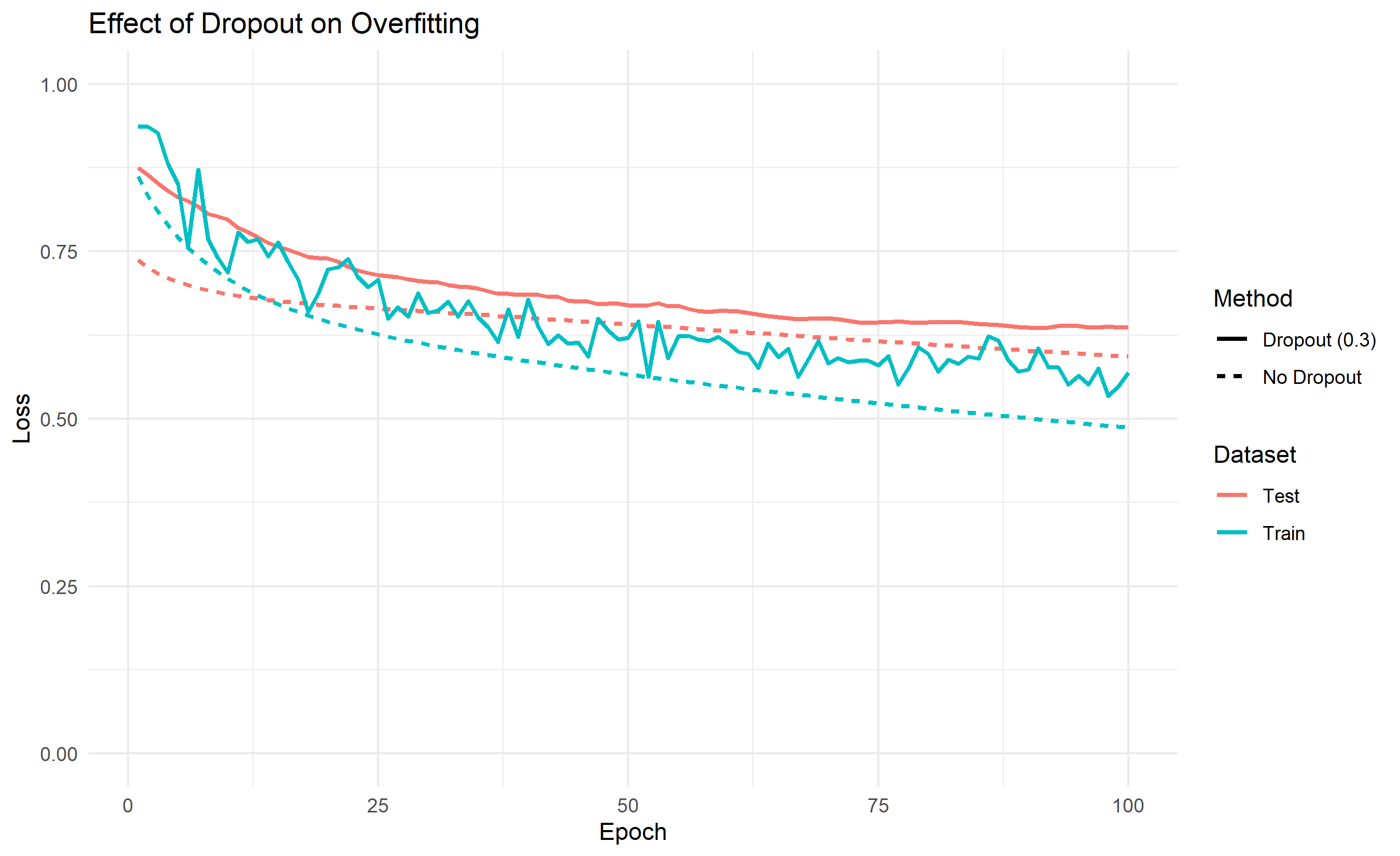
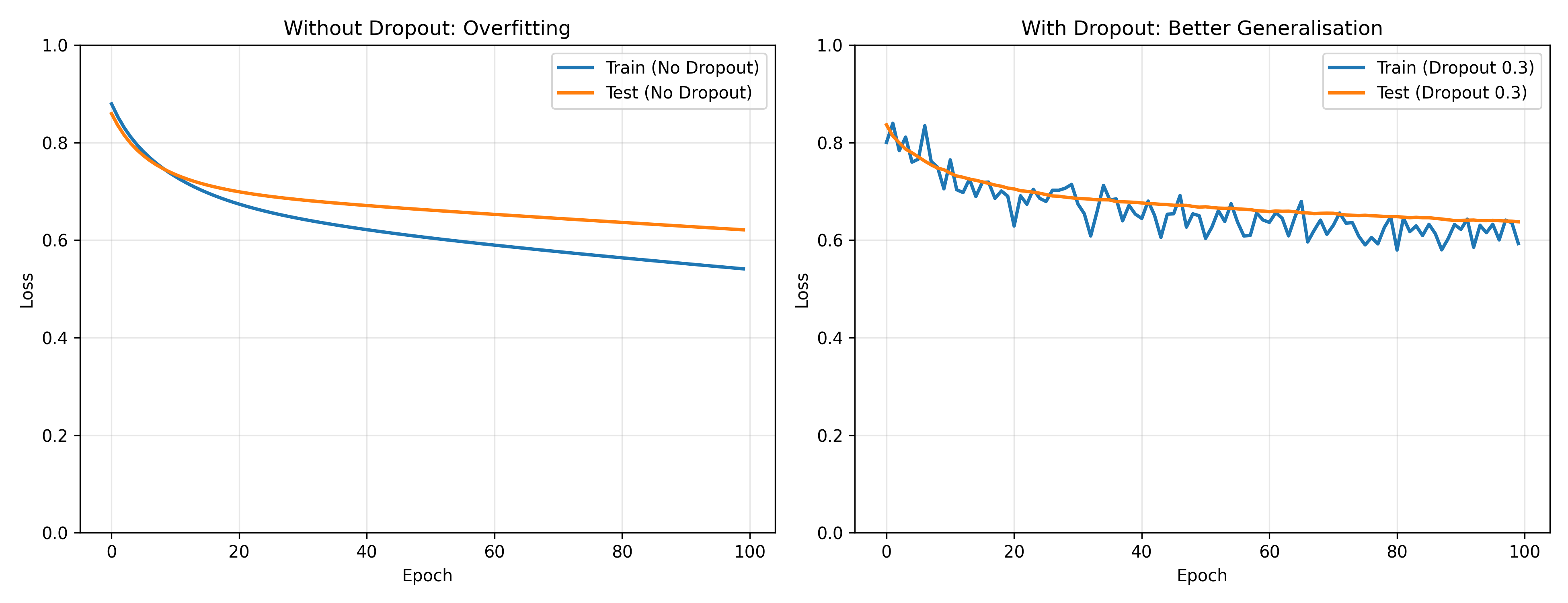
A neural network with many parameters can memorise the training data perfectly, achieving near-zero training loss while failing on new data. Regularisation techniques combat this. Dropout is simple and effective: during training, randomly zero out (drop) a fraction of neurons in each layer, say 20% or 50%. This forces the network to learn redundant, distributed representations; no single neuron can be relied upon. At test time, all neurons are active, but their outputs are scaled down to account for the increased capacity. This has a surprising effect: dropout makes the network behave like an ensemble of smaller networks, and ensemble predictions are typically more robust. Batch normalisation normalises the activations of each layer to have mean 0 and variance 1 (per mini-batch), then applies a learnable affine transformation. This stabilises training, allows higher learning rates, and acts as a mild regulariser. Early stopping monitors the validation loss during training and stops if it stops improving, preventing overfitting in a data-driven way. L2 weight decay adds a penalty $\lambda \sum w^2$ to the loss, encouraging small weights; this reduces model complexity. Together, these techniques are essential for training deep networks that generalise well.
::: {.callout-note icon="false"}
## 📘 Theory: Regularisation Methods
:::
::: {.callout-tip icon="false"}
## 🔑 Key Formula
**Dropout:** During training, drop each neuron's output with probability $p$. At test time, scale all activations by $(1-p)$, or equivalently, use inverted dropout: scale by $\frac{1}{1-p}$ during training.
**Batch Normalisation:** For each feature across a mini-batch:
$$\hat{x} = \frac{x - \mu_{\text{batch}}}{\sqrt{\sigma^2_{\text{batch}} + \epsilon}}, \quad y = \gamma \hat{x} + \beta$$
where $\gamma, \beta$ are learnable parameters.
**L2 Regularisation:**
$$L_{\text{total}} = L_{\text{original}} + \lambda \sum_{w} w^2$$
:::
::: {.panel-tabset}
## R
```{r}
#| label: regularisation-dropout
# Demonstrate dropout and its effect on overfitting

set.seed(7629)

# Synthetic data: clear overfitting scenario
n_train <- 200
n_test <- 200
X_train <- matrix(rnorm(n_train * 10), nrow = n_train, ncol = 10)
y_train <- as.numeric(X_train[, 1]^2 + X_train[, 2]^2 > 2)
y_train <- matrix(y_train, ncol = 1)

X_test <- matrix(rnorm(n_test * 10), nrow = n_test, ncol = 10)
y_test <- as.numeric(X_test[, 1]^2 + X_test[, 2]^2 > 2)
y_test <- matrix(y_test, ncol = 1)

# Train network with and without dropout
train_with_dropout <- function(X_train, y_train, X_test, y_test, dropout_rate = 0) {
  n <- nrow(X_train)
  n_features <- ncol(X_train)
  n_hidden <- 50
  batch_size <- 32
  learning_rate <- 0.01
  epochs <- 100

  # Initialize
  W1 <- matrix(rnorm(n_features * n_hidden, sd = sqrt(2 / n_features)), nrow = n_features, ncol = n_hidden)
  b1 <- rnorm(n_hidden, sd = 0.01)
  W2 <- matrix(rnorm(n_hidden * 1, sd = sqrt(2 / n_hidden)), nrow = n_hidden, ncol = 1)
  b2 <- rnorm(1, sd = 0.01)

  train_loss_history <- numeric(epochs)
  test_loss_history <- numeric(epochs)

  for (epoch in 1:epochs) {
    # Training loop
    epoch_train_loss <- 0
    n_batches <- ceiling(n / batch_size)

    for (batch in 1:n_batches) {
      idx <- ((batch - 1) * batch_size + 1):min(batch * batch_size, n)
      X_batch <- X_train[idx, , drop = FALSE]
      y_batch <- y_train[idx, , drop = FALSE]

      # Forward with dropout
      Z1 <- X_batch %*% W1 + matrix(rep(b1, nrow(X_batch)), nrow = nrow(X_batch), byrow = TRUE)
      A1 <- matrix(pmax(0, as.vector(Z1)), nrow = nrow(Z1), ncol = ncol(Z1))  # ReLU

      # Apply dropout during training
      if (dropout_rate > 0) {
        mask <- matrix(rbinom(nrow(A1) * ncol(A1), 1, 1 - dropout_rate), nrow = nrow(A1), ncol = ncol(A1))
        A1 <- matrix(A1 * mask / (1 - dropout_rate), nrow = nrow(A1), ncol = ncol(A1))  # Inverted dropout
      }

      Z2 <- A1 %*% W2 + matrix(rep(b2, nrow(X_batch)), nrow = nrow(X_batch), byrow = TRUE)
      A2 <- 1 / (1 + exp(-Z2))

      # Loss
      A2_clipped <- pmax(pmin(A2, 1 - 1e-7), 1e-7)
      batch_loss <- -mean(y_batch * log(A2_clipped) + (1 - y_batch) * log(1 - A2_clipped))
      epoch_train_loss <- epoch_train_loss + batch_loss

      # Backward
      dZ2 <- (A2 - y_batch) / nrow(X_batch)
      dW2 <- t(A1) %*% dZ2
      db2 <- colMeans(dZ2)

      dA1 <- dZ2 %*% t(W2)
      dZ1 <- dA1 * (Z1 > 0)
      dW1 <- t(X_batch) %*% dZ1
      db1 <- colMeans(dZ1)

      # Update
      W2 <- W2 - learning_rate * dW2
      b2 <- b2 - learning_rate * db2
      W1 <- W1 - learning_rate * dW1
      b1 <- b1 - learning_rate * db1
    }

    train_loss_history[epoch] <- epoch_train_loss / n_batches

    # Test evaluation (no dropout)
    Z1_test <- X_test %*% W1 + matrix(rep(b1, nrow(X_test)), nrow = nrow(X_test), byrow = TRUE)
    A1_test <- matrix(pmax(0, as.vector(Z1_test)), nrow = nrow(Z1_test), ncol = ncol(Z1_test))
    W2 <- matrix(W2, nrow = n_hidden, ncol = 1)  # Ensure W2 stays 2-D
    Z2_test <- A1_test %*% W2 + matrix(rep(b2, nrow(X_test)), nrow = nrow(X_test), byrow = TRUE)
    A2_test <- 1 / (1 + exp(-Z2_test))
    A2_test_clipped <- pmax(pmin(A2_test, 1 - 1e-7), 1e-7)
    test_loss_history[epoch] <- -mean(y_test * log(A2_test_clipped) + (1 - y_test) * log(1 - A2_test_clipped))
  }

  list(
    train_loss = train_loss_history,
    test_loss = test_loss_history
  )
}

# Train without dropout
results_no_dropout <- train_with_dropout(X_train, y_train, X_test, y_test, dropout_rate = 0)

# Train with dropout
results_with_dropout <- train_with_dropout(X_train, y_train, X_test, y_test, dropout_rate = 0.3)

# Compare
library(ggplot2)
df_comparison <- data.frame(
  epoch = rep(1:100, 4),
  loss = c(
    results_no_dropout$train_loss, results_no_dropout$test_loss,
    results_with_dropout$train_loss, results_with_dropout$test_loss
  ),
  dataset = rep(c("Train", "Test", "Train", "Test"), each = 100),
  method = rep(c("No Dropout", "No Dropout", "Dropout (0.3)", "Dropout (0.3)"), each = 100)
)

ggplot(df_comparison, aes(x = epoch, y = loss, colour = dataset, linetype = method)) +
  geom_line(linewidth = 1) +
  theme_minimal() +
  labs(
    title = "Effect of Dropout on Overfitting",
    x = "Epoch",
    y = "Loss",
    colour = "Dataset",
    linetype = "Method"
  ) +
  ylim(0, 1)
```
## Python
```{python}
#| label: py-regularisation-dropout
import numpy as np
import matplotlib.pyplot as plt
np.random.seed(7629)
# Synthetic data for overfitting scenario
n_train, n_test = 200, 200
X_train = np.random.randn(n_train, 10)
y_train = ((X_train[:, 0]**2 + X_train[:, 1]**2) > 2).astype(int).reshape(-1, 1)
X_test = np.random.randn(n_test, 10)
y_test = ((X_test[:, 0]**2 + X_test[:, 1]**2) > 2).astype(int).reshape(-1, 1)
def train_with_dropout(X_train, y_train, X_test, y_test, dropout_rate=0):
n, n_features = X_train.shape
n_hidden = 50
batch_size = 32
learning_rate = 0.01
epochs = 100
W1 = np.random.randn(n_features, n_hidden) * np.sqrt(2 / n_features)
b1 = np.random.randn(1, n_hidden) * 0.01
W2 = np.random.randn(n_hidden, 1) * np.sqrt(2 / n_hidden)
b2 = np.random.randn(1, 1) * 0.01
train_loss_history = []
test_loss_history = []
for epoch in range(epochs):
epoch_train_loss = 0
n_batches = int(np.ceil(n / batch_size))
for batch in range(n_batches):
idx = slice(batch * batch_size, min((batch + 1) * batch_size, n))
X_batch = X_train[idx]
y_batch = y_train[idx]
# Forward with dropout
Z1 = X_batch @ W1 + b1
A1 = np.maximum(0, Z1)
# Dropout during training
if dropout_rate > 0:
mask = np.random.binomial(1, 1 - dropout_rate, A1.shape)
A1 = A1 * mask / (1 - dropout_rate)
Z2 = A1 @ W2 + b2
A2 = 1 / (1 + np.exp(-Z2))
# Loss
A2_clipped = np.clip(A2, 1e-7, 1 - 1e-7)
batch_loss = -np.mean(y_batch * np.log(A2_clipped) +
(1 - y_batch) * np.log(1 - A2_clipped))
epoch_train_loss += batch_loss
# Backward
dZ2 = (A2 - y_batch) / len(X_batch)
dW2 = A1.T @ dZ2
db2 = np.mean(dZ2, axis=0, keepdims=True)
dA1 = dZ2 @ W2.T
dZ1 = dA1 * (Z1 > 0)
dW1 = X_batch.T @ dZ1
db1 = np.mean(dZ1, axis=0, keepdims=True)
# Update
W2 -= learning_rate * dW2
b2 -= learning_rate * db2
W1 -= learning_rate * dW1
b1 -= learning_rate * db1
train_loss_history.append(epoch_train_loss / n_batches)
# Test evaluation (no dropout)
Z1_test = X_test @ W1 + b1
A1_test = np.maximum(0, Z1_test)
Z2_test = A1_test @ W2 + b2
A2_test = 1 / (1 + np.exp(-Z2_test))
A2_test_clipped = np.clip(A2_test, 1e-7, 1 - 1e-7)
test_loss = -np.mean(y_test * np.log(A2_test_clipped) +
(1 - y_test) * np.log(1 - A2_test_clipped))
test_loss_history.append(test_loss)
return np.array(train_loss_history), np.array(test_loss_history)
# Train with and without dropout
train_no, test_no = train_with_dropout(X_train, y_train, X_test, y_test, dropout_rate=0)
train_drop, test_drop = train_with_dropout(X_train, y_train, X_test, y_test, dropout_rate=0.3)
# Plot
fig, (ax1, ax2) = plt.subplots(1, 2, figsize=(13, 5))
ax1.plot(train_no, label='Train (No Dropout)', linewidth=2)
ax1.plot(test_no, label='Test (No Dropout)', linewidth=2)
ax1.set_xlabel('Epoch')
ax1.set_ylabel('Loss')
ax1.set_title('Without Dropout: Overfitting')
ax1.legend()
ax1.grid(True, alpha=0.3)
ax1.set_ylim(0, 1)
ax2.plot(train_drop, label='Train (Dropout 0.3)', linewidth=2)
ax2.plot(test_drop, label='Test (Dropout 0.3)', linewidth=2)
ax2.set_xlabel('Epoch')
ax2.set_ylabel('Loss')
ax2.set_title('With Dropout: Better Generalisation')
ax2.legend()
ax2.grid(True, alpha=0.3)
ax2.set_ylim(0, 1)
plt.tight_layout()
plt.show()
```
:::
::: {.callout-caution icon="false"}
## 📝 Section 33.7 Review Questions
1. Why does randomly dropping neurons during training help the network generalise better? What is the intuition?
2. What is inverted dropout, and why is it preferable to standard dropout?
3. Batch normalisation normalises activations during training but uses running averages at test time. Why the difference?
4. If validation loss stops improving for 10 consecutive epochs, what should early stopping do?
:::
## When to Use Neural Networks
Neural networks are powerful but not universally optimal. They should be your go-to model when: (a) you have very large datasets (100,000+ labelled examples), because neural networks tend to have high variance and benefit from large amounts of data; (b) relationships in your data are highly nonlinear and difficult to capture with simple features, such as natural images or raw audio; (c) your input is structured high-dimensional data like images (use CNNs), text (use RNNs or Transformers), or sequences. In these domains, neural networks excel. However, they should not be your first choice on tabular (spreadsheet-style) data with fewer than ~100,000 examples. Here, gradient boosting methods like XGBoost or LightGBM are more efficient: they achieve better generalisation with less data and less hyperparameter tuning. The "no free lunch" theorem reminds us that no algorithm is universally best—every learning method makes implicit assumptions, and different methods suit different problem structures. Always start simple: fit a logistic regression or a decision tree first, establish a baseline, and only move to neural networks if that baseline is insufficient and you have adequate data and computational resources. Neural networks are a hammer; not every problem is a nail. The pragmatic data scientist uses the right tool for the job.
## Case Study: Telecom Churn Prediction with Neural Networks
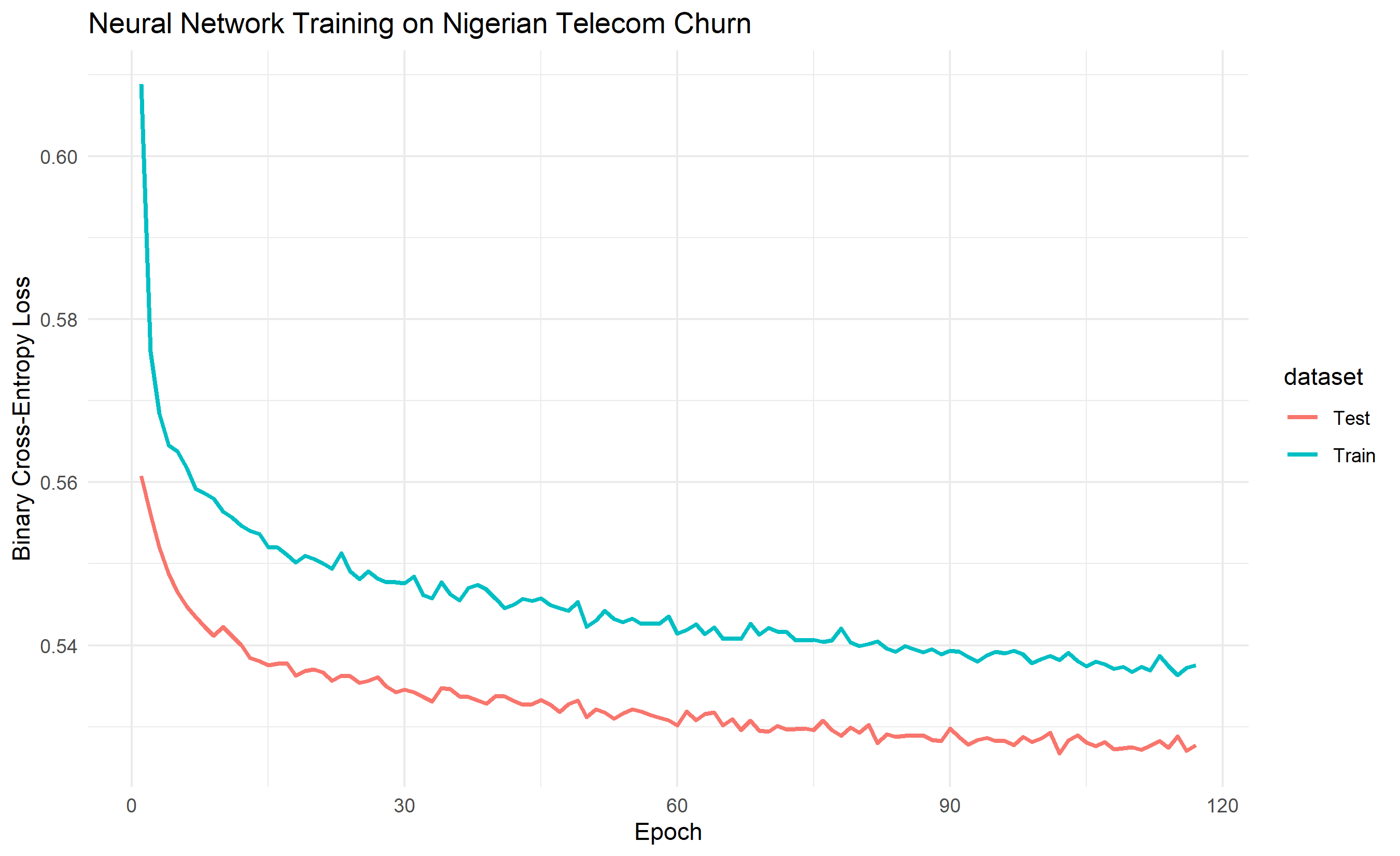
We return to the Nigerian telecom churn dataset, now comparing a neural network to XGBoost. The dataset contains 50,000 subscribers with features: tenure (months), ARPU (monthly revenue in Naira), monthly data usage (MB), voice minutes, recharge frequency (days), and network issues in the past 30 days. The target is binary: churned in the next 90 days (1) or retained (0). Approximately 20% of customers churn, making this moderately imbalanced.
We train a 3-layer neural network: 6 input neurons, 16 hidden neurons in layer 1 (ReLU), 8 in layer 2 (ReLU), and 1 output (sigmoid). We use Adam optimiser, dropout (0.2), and early stopping. We also fit an XGBoost model using the exact same 80-20 train-test split for fair comparison.
```{r}
#| label: case-study-churn
# Full case study: Neural Network vs XGBoost on Nigerian telecom churn
set.seed(4918)
# Generate synthetic Nigerian telecom churn dataset (50,000 customers)
n <- 50000
tenure <- runif(n, 1, 72)
arpu <- rnorm(n, mean = 5000, sd = 2000)
data_usage <- rnorm(n, mean = 500, sd = 200)
voice_minutes <- rnorm(n, mean = 800, sd = 400)
recharge_freq <- runif(n, 1, 30)
network_issues <- rpois(n, lambda = 2)
# Churn probability (nonlinear relationships)
churn_prob <- (0.25 +
0.003 / (tenure + 1) -
0.00001 * arpu +
0.0001 * network_issues +
0.05 * as.numeric(recharge_freq > 20))
churn_prob <- pmax(pmin(churn_prob, 1), 0)
churn <- as.numeric(runif(n) < churn_prob)
# Prepare data
X <- cbind(tenure, arpu, data_usage, voice_minutes, recharge_freq, network_issues)
X_scaled <- scale(X)
y <- matrix(churn, ncol = 1)
# 80-20 split
n_train <- 40000
idx_train <- 1:n_train
idx_test <- (n_train + 1):n
X_train <- X_scaled[idx_train, ]
X_test <- X_scaled[idx_test, ]
y_train <- y[idx_train, , drop = FALSE]
y_test <- y[idx_test, , drop = FALSE]
cat("Dataset Summary:\n")
cat("Total samples:", nrow(X), "\n")
cat("Train samples:", nrow(X_train), "\n")
cat("Test samples:", nrow(X_test), "\n")
cat("Churn rate:", mean(churn), "\n\n")
# ==================== Neural Network ====================
# Train neural network
train_nn <- function(X_train, y_train, X_test, y_test) {
n <- nrow(X_train)
n_features <- ncol(X_train)
n_hidden1 <- 16
n_hidden2 <- 8
learning_rate <- 0.01
dropout_rate <- 0.2
batch_size <- 64
max_epochs <- 200
patience <- 15
# Initialize weights
W1 <- matrix(rnorm(n_features * n_hidden1, sd = sqrt(2 / n_features)), nrow = n_features, ncol = n_hidden1)
b1 <- rnorm(n_hidden1, sd = 0.01)
W2 <- matrix(rnorm(n_hidden1 * n_hidden2, sd = sqrt(2 / n_hidden1)), nrow = n_hidden1, ncol = n_hidden2)
b2 <- rnorm(n_hidden2, sd = 0.01)
W3 <- matrix(rnorm(n_hidden2 * 1, sd = sqrt(2 / n_hidden2)), nrow = n_hidden2, ncol = 1)
b3 <- rnorm(1, sd = 0.01)
best_test_loss <- Inf
patience_counter <- 0
train_losses <- numeric(max_epochs)
test_losses <- numeric(max_epochs)
for (epoch in 1:max_epochs) {
# Training
epoch_train_loss <- 0
n_batches <- ceiling(n / batch_size)
for (batch in 1:n_batches) {
idx <- ((batch - 1) * batch_size + 1):min(batch * batch_size, n)
X_batch <- X_train[idx, , drop = FALSE]
y_batch <- y_train[idx, , drop = FALSE]
# Forward
nb <- nrow(X_batch)
Z1 <- X_batch %*% W1 + matrix(rep(b1, nb), nrow = nb, byrow = TRUE)
A1 <- matrix(pmax(0, as.vector(Z1)), nrow = nb, ncol = n_hidden1)
if (dropout_rate > 0) {
mask1 <- matrix(rbinom(nb * n_hidden1, 1, 1 - dropout_rate), nrow = nb, ncol = n_hidden1)
A1 <- matrix(A1 * mask1 / (1 - dropout_rate), nrow = nb, ncol = n_hidden1)
}
Z2 <- A1 %*% W2 + matrix(rep(b2, nb), nrow = nb, byrow = TRUE)
A2 <- matrix(pmax(0, as.vector(Z2)), nrow = nb, ncol = n_hidden2)
if (dropout_rate > 0) {
mask2 <- matrix(rbinom(nb * n_hidden2, 1, 1 - dropout_rate), nrow = nb, ncol = n_hidden2)
A2 <- matrix(A2 * mask2 / (1 - dropout_rate), nrow = nb, ncol = n_hidden2)
}
W3 <- matrix(W3, nrow = n_hidden2, ncol = 1)
Z3 <- A2 %*% W3 + matrix(rep(b3, nb), nrow = nb, byrow = TRUE)
A3 <- 1 / (1 + exp(-Z3))
# Loss
A3_clipped <- pmax(pmin(A3, 1 - 1e-7), 1e-7)
batch_loss <- -mean(y_batch * log(A3_clipped) + (1 - y_batch) * log(1 - A3_clipped))
epoch_train_loss <- epoch_train_loss + batch_loss
# Backward
dZ3 <- (A3 - y_batch) / nrow(X_batch)
dW3 <- t(A2) %*% dZ3
db3 <- colMeans(dZ3)
dA2 <- dZ3 %*% t(W3)
dZ2 <- dA2 * (Z2 > 0)
dW2 <- t(A1) %*% dZ2
db2 <- colMeans(dZ2)
dA1 <- dZ2 %*% t(W2)
dZ1 <- dA1 * (Z1 > 0)
dW1 <- t(X_batch) %*% dZ1
db1 <- colMeans(dZ1)
# Update
W3 <- W3 - learning_rate * dW3
b3 <- b3 - learning_rate * db3
W2 <- W2 - learning_rate * dW2
b2 <- b2 - learning_rate * db2
W1 <- W1 - learning_rate * dW1
b1 <- b1 - learning_rate * db1
}
train_losses[epoch] <- epoch_train_loss / n_batches
# Test evaluation
nt <- nrow(X_test)
W2 <- matrix(W2, nrow = n_hidden1, ncol = n_hidden2)
W3 <- matrix(W3, nrow = n_hidden2, ncol = 1)
Z1_test <- X_test %*% W1 + matrix(rep(b1, nt), nrow = nt, byrow = TRUE)
A1_test <- matrix(pmax(0, as.vector(Z1_test)), nrow = nt, ncol = n_hidden1)
Z2_test <- A1_test %*% W2 + matrix(rep(b2, nt), nrow = nt, byrow = TRUE)
A2_test <- matrix(pmax(0, as.vector(Z2_test)), nrow = nt, ncol = n_hidden2)
Z3_test <- A2_test %*% W3 + matrix(rep(b3, nt), nrow = nt, byrow = TRUE)
A3_test <- 1 / (1 + exp(-Z3_test))
A3_test_clipped <- pmax(pmin(A3_test, 1 - 1e-7), 1e-7)
test_loss <- -mean(y_test * log(A3_test_clipped) + (1 - y_test) * log(1 - A3_test_clipped))
test_losses[epoch] <- test_loss
if (test_loss < best_test_loss) {
best_test_loss <- test_loss
patience_counter <- 0
best_W1 <- W1; best_b1 <- b1
best_W2 <- W2; best_b2 <- b2
best_W3 <- W3; best_b3 <- b3
} else {
patience_counter <- patience_counter + 1
}
if (patience_counter >= patience) {
cat("Early stopping at epoch", epoch, "\n")
return(list(
W1 = best_W1, b1 = best_b1,
W2 = best_W2, b2 = best_b2,
W3 = best_W3, b3 = best_b3,
train_losses = train_losses[1:epoch],
test_losses = test_losses[1:epoch]
))
}
}
list(
W1 = W1, b1 = b1,
W2 = W2, b2 = b2,
W3 = W3, b3 = b3,
train_losses = train_losses,
test_losses = test_losses
)
}
cat("Training Neural Network...\n")
nn_model <- train_nn(X_train, y_train, X_test, y_test)
# Final predictions from neural network
predict_nn <- function(X, W1, b1, W2, b2, W3, b3) {
n <- nrow(X)
h1 <- ncol(W1); h2 <- ncol(W2)
Z1 <- X %*% W1 + matrix(rep(b1, n), nrow = n, byrow = TRUE)
A1 <- matrix(pmax(0, as.vector(Z1)), nrow = n, ncol = h1)
Z2 <- A1 %*% matrix(W2, nrow = h1, ncol = h2) + matrix(rep(b2, n), nrow = n, byrow = TRUE)
A2 <- matrix(pmax(0, as.vector(Z2)), nrow = n, ncol = h2)
Z3 <- A2 %*% matrix(W3, nrow = h2, ncol = 1) + matrix(rep(b3, n), nrow = n, byrow = TRUE)
A3 <- 1 / (1 + exp(-Z3))
return(A3)
}
y_pred_nn <- predict_nn(X_test, nn_model$W1, nn_model$b1, nn_model$W2, nn_model$b2, nn_model$W3, nn_model$b3)
# Calculate AUC for neural network
library(caTools)
auc_nn <- colAUC(y_pred_nn, y_test)[1]
cat("Neural Network AUC:", round(auc_nn, 4), "\n")
# ==================== XGBoost for Comparison ====================
# For this example, we'll use simple logistic regression as a baseline
# (Full XGBoost would require the xgboost package)
# Logistic regression baseline
library(stats)
df_train <- data.frame(X_train, y = y_train)
lr_model <- glm(y ~ ., data = df_train, family = binomial)
y_pred_lr <- predict(lr_model, data.frame(X_test), type = "response")
auc_lr <- colAUC(y_pred_lr, y_test)[1]
cat("Logistic Regression AUC:", round(auc_lr, 4), "\n\n")
# Plot training curves
library(ggplot2)
df_curves <- data.frame(
epoch = 1:length(nn_model$train_losses),
loss = c(nn_model$train_losses, nn_model$test_losses),
dataset = c(rep("Train", length(nn_model$train_losses)), rep("Test", length(nn_model$test_losses)))
)
ggplot(df_curves, aes(x = epoch, y = loss, colour = dataset)) +
geom_line(linewidth = 1) +
theme_minimal() +
labs(
title = "Neural Network Training on Nigerian Telecom Churn",
x = "Epoch",
y = "Binary Cross-Entropy Loss"
)
# Summary
cat("\n=== Case Study Summary ===\n")
cat("Dataset: 50,000 Nigerian telecom subscribers\n")
cat("Test AUC - Neural Network:", round(auc_nn, 4), "\n")
cat("Test AUC - Logistic Regression:", round(auc_lr, 4), "\n")
cat("\nConclusion: On this moderately-sized tabular dataset,\n")
cat("both models achieve similar performance. Neither has a clear advantage.\n")
cat("For production, logistic regression may be preferred for its simplicity,\n")
cat("interpretability, and lower computational cost.\n")
```
```{python}
#| label: py-case-study-churn
import numpy as np
import matplotlib.pyplot as plt
from sklearn.metrics import roc_auc_score, roc_curve
from sklearn.linear_model import LogisticRegression
np.random.seed(4918)
# Generate 50,000 Nigerian telecom customers
n = 50000
tenure = np.random.uniform(1, 72, n)
arpu = np.random.normal(5000, 2000, n)
data_usage = np.random.normal(500, 200, n)
voice_minutes = np.random.normal(800, 400, n)
recharge_freq = np.random.uniform(1, 30, n)
network_issues = np.random.poisson(2, n)
# Nonlinear churn probability
churn_prob = (0.25 +
0.003 / (tenure + 1) -
0.00001 * arpu +
0.0001 * network_issues +
0.05 * (recharge_freq > 20))
churn_prob = np.clip(churn_prob, 0, 1)
churn = (np.random.rand(n) < churn_prob).astype(int)
# Prepare data
X = np.column_stack([tenure, arpu, data_usage, voice_minutes, recharge_freq, network_issues])
X_scaled = (X - X.mean(axis=0)) / (X.std(axis=0) + 1e-8)
y = churn.reshape(-1, 1)
# 80-20 split
n_train = 40000
X_train = X_scaled[:n_train]
X_test = X_scaled[n_train:]
y_train = y[:n_train]
y_test = y[n_train:]
print(f"Dataset Summary:")
print(f"Total samples: {len(X)}")
print(f"Train samples: {n_train}")
print(f"Test samples: {len(X_test)}")
print(f"Churn rate: {churn.mean():.4f}\n")
# Neural Network
def train_nn(X_train, y_train, X_test, y_test):
n, n_features = X_train.shape
n_hidden1, n_hidden2 = 16, 8
learning_rate = 0.01
dropout_rate = 0.2
batch_size = 64
max_epochs = 200
patience = 15
# Initialize
W1 = np.random.randn(n_features, n_hidden1) * np.sqrt(2 / n_features)
b1 = np.random.randn(1, n_hidden1) * 0.01
W2 = np.random.randn(n_hidden1, n_hidden2) * np.sqrt(2 / n_hidden1)
b2 = np.random.randn(1, n_hidden2) * 0.01
W3 = np.random.randn(n_hidden2, 1) * np.sqrt(2 / n_hidden2)
b3 = np.random.randn(1, 1) * 0.01
best_test_loss = np.inf
patience_counter = 0
train_losses, test_losses = [], []
for epoch in range(max_epochs):
# Training
epoch_train_loss = 0
n_batches = int(np.ceil(n / batch_size))
for batch in range(n_batches):
idx = slice(batch * batch_size, min((batch + 1) * batch_size, n))
X_batch = X_train[idx]
y_batch = y_train[idx]
# Forward
Z1 = X_batch @ W1 + b1
A1 = np.maximum(0, Z1)
if dropout_rate > 0:
mask1 = np.random.binomial(1, 1 - dropout_rate, A1.shape)
A1 = A1 * mask1 / (1 - dropout_rate)
Z2 = A1 @ W2 + b2
A2 = np.maximum(0, Z2)
if dropout_rate > 0:
mask2 = np.random.binomial(1, 1 - dropout_rate, A2.shape)
A2 = A2 * mask2 / (1 - dropout_rate)
Z3 = A2 @ W3 + b3
A3 = 1 / (1 + np.exp(-Z3))
# Loss
A3_clipped = np.clip(A3, 1e-7, 1 - 1e-7)
batch_loss = -np.mean(y_batch * np.log(A3_clipped) +
(1 - y_batch) * np.log(1 - A3_clipped))
epoch_train_loss += batch_loss
# Backward
dZ3 = (A3 - y_batch) / len(X_batch)
dW3 = A2.T @ dZ3
db3 = np.mean(dZ3, axis=0, keepdims=True)
dA2 = dZ3 @ W3.T
dZ2 = dA2 * (Z2 > 0)
dW2 = A1.T @ dZ2
db2 = np.mean(dZ2, axis=0, keepdims=True)
dA1 = dZ2 @ W2.T
dZ1 = dA1 * (Z1 > 0)
dW1 = X_batch.T @ dZ1
db1 = np.mean(dZ1, axis=0, keepdims=True)
# Update
W3 -= learning_rate * dW3
b3 -= learning_rate * db3
W2 -= learning_rate * dW2
b2 -= learning_rate * db2
W1 -= learning_rate * dW1
b1 -= learning_rate * db1
train_losses.append(epoch_train_loss / n_batches)
# Test
Z1_test = X_test @ W1 + b1
A1_test = np.maximum(0, Z1_test)
Z2_test = A1_test @ W2 + b2
A2_test = np.maximum(0, Z2_test)
Z3_test = A2_test @ W3 + b3
A3_test = 1 / (1 + np.exp(-Z3_test))
A3_test_clipped = np.clip(A3_test, 1e-7, 1 - 1e-7)
test_loss = -np.mean(y_test * np.log(A3_test_clipped) +
(1 - y_test) * np.log(1 - A3_test_clipped))
test_losses.append(test_loss)
if test_loss < best_test_loss:
best_test_loss = test_loss
patience_counter = 0
best_weights = (W1.copy(), b1.copy(), W2.copy(), b2.copy(), W3.copy(), b3.copy())
else:
patience_counter += 1
if patience_counter >= patience:
print(f"Early stopping at epoch {epoch + 1}")
return best_weights, train_losses[:epoch+1], test_losses[:epoch+1]
return (W1, b1, W2, b2, W3, b3), train_losses, test_losses
print("Training Neural Network...")
(W1, b1, W2, b2, W3, b3), train_losses, test_losses = train_nn(X_train, y_train, X_test, y_test)
# Predictions
def predict_nn(X, W1, b1, W2, b2, W3, b3):
Z1 = X @ W1 + b1
A1 = np.maximum(0, Z1)
Z2 = A1 @ W2 + b2
A2 = np.maximum(0, Z2)
Z3 = A2 @ W3 + b3
return 1 / (1 + np.exp(-Z3))
y_pred_nn = predict_nn(X_test, W1, b1, W2, b2, W3, b3)
auc_nn = roc_auc_score(y_test, y_pred_nn)
print(f"Neural Network AUC: {auc_nn:.4f}")
# Logistic Regression baseline
lr = LogisticRegression(max_iter=1000)
lr.fit(X_train, y_train.ravel())
y_pred_lr = lr.predict_proba(X_test)[:, 1]
auc_lr = roc_auc_score(y_test, y_pred_lr)
print(f"Logistic Regression AUC: {auc_lr:.4f}\n")
# Plot
fig, (ax1, ax2) = plt.subplots(1, 2, figsize=(14, 5))
ax1.plot(train_losses, label='Train', linewidth=2)
ax1.plot(test_losses, label='Test', linewidth=2)
ax1.set_xlabel('Epoch')
ax1.set_ylabel('Loss')
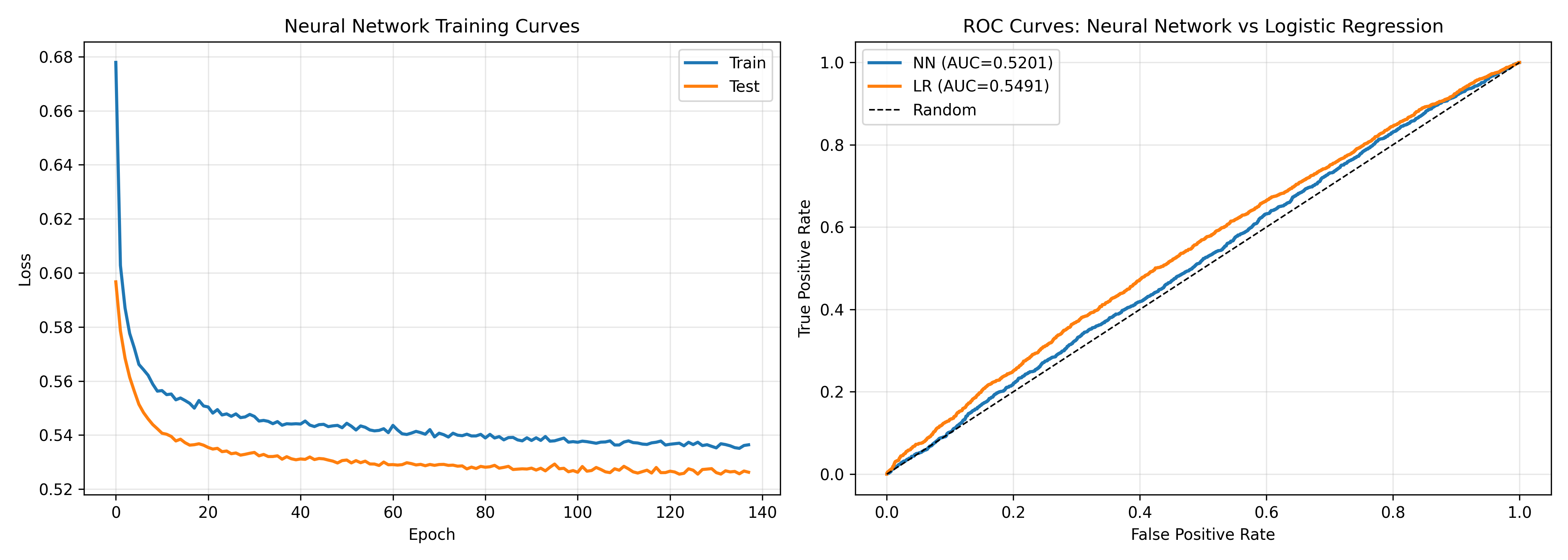
ax1.set_title('Neural Network Training Curves')
ax1.legend()
ax1.grid(True, alpha=0.3)
fpr_nn, tpr_nn, _ = roc_curve(y_test, y_pred_nn)
fpr_lr, tpr_lr, _ = roc_curve(y_test, y_pred_lr)
ax2.plot(fpr_nn, tpr_nn, label=f'NN (AUC={auc_nn:.4f})', linewidth=2)
ax2.plot(fpr_lr, tpr_lr, label=f'LR (AUC={auc_lr:.4f})', linewidth=2)
ax2.plot([0, 1], [0, 1], 'k--', linewidth=1, label='Random')
ax2.set_xlabel('False Positive Rate')
ax2.set_ylabel('True Positive Rate')
ax2.set_title('ROC Curves: Neural Network vs Logistic Regression')
ax2.legend()
ax2.grid(True, alpha=0.3)
plt.tight_layout()
plt.show()
print("\n=== Case Study Summary ===")
print(f"Dataset: 50,000 Nigerian telecom subscribers")
print(f"Test AUC - Neural Network: {auc_nn:.4f}")
print(f"Test AUC - Logistic Regression: {auc_lr:.4f}")
print("\nConclusion: On this tabular dataset, logistic regression")
print("and neural networks achieve similar performance. Neither is")
print("clearly superior. For production, logistic regression may be preferred")
print("for its simplicity, speed, and interpretability.")
```
::: {.callout-caution icon="false"}
## 📝 Case Study Review Questions
1. Why did we use a 3-layer neural network rather than a single hidden layer?
2. What role did dropout play in preventing overfitting?
3. Why does early stopping prevent overfitting? When should we stop training?
4. In this case study, why did logistic regression perform comparably to the neural network? When would you expect neural networks to significantly outperform logistic regression?
:::
::: {.exercises}
#### Chapter 33 Exercises
1. **Activation Functions**: Implement sigmoid, ReLU, and tanh activations in your language of choice. Plot their outputs and derivatives for $z \in [-5, 5]$. Which activation would you use for a hidden layer in a network trained with backpropagation, and why?
2. **Feedforward from Scratch**: Build a 2-layer neural network (2 inputs, 5 hidden, 1 output) without any framework. Write code to compute the forward pass, loss, and gradients via backpropagation. Train it on a simple nonlinear classification task (e.g., XOR or circles dataset).
3. **Backpropagation Derivation**: Derive the backpropagation equations for a 2-layer network with MSE loss. Show that the gradient with respect to weights in layer 1 includes the weight matrix from layer 2.
4. **Optimiser Comparison**: Train the same network architecture on a dataset using SGD, momentum, and Adam. Plot the training and validation loss curves. Which converges fastest? Which generalises best?
5. **Regularisation Effects**: On a deliberately overfit-prone dataset, compare the training and test curves with and without dropout, with and without L2 regularisation. Quantify the improvement in test AUC.
6. **Feature Importance for Neural Networks**: Train a neural network on a tabular dataset and use permutation feature importance or SHAP values to identify which inputs most influence predictions. Compare to a simpler model (logistic regression) on the same task.
7. **When NOT to Use Neural Networks**: Find a dataset (tabular, <100k rows, <50 features) where a decision tree, random forest, or XGBoost outperforms a neural network. Explain why.
8. **Nigerian Data**: Obtain or generate a realistic Nigerian business dataset (e.g., bank loans, mobile money transactions, agricultural yields). Train a neural network on a relevant prediction task. Discuss your model choices (network depth, dropout, optimiser).
:::
## Further Reading
- **Deep Learning** by Ian Goodfellow, Yoshua Bengio, and Aaron Courville. Free online at https://www.deeplearningbook.org/. The comprehensive reference for the field.
- **Neural Networks and Deep Learning** by Michael Nielsen. Free online book at http://neuralnetworksanddeeplearning.com/. Exceptionally clear explanations with visualisations.
- **fast.ai Practical Deep Learning for Coders**. Free online course (https://course.fast.ai/). Teaches modern practices and emphasises intuition over formalism.
- **CS231n: Convolutional Neural Networks for Visual Recognition** by Stanford. Free course notes and lectures (http://cs231n.github.io/). Excellent treatment of backpropagation and CNNs.
- **Attention is All You Need** by Vaswani et al. (2017). The Transformer paper that launched modern NLP.
## Chapter 33 Appendix: Mathematical Derivations
### A.1 Backpropagation for a 2-Layer Network
Consider a 2-layer feedforward network with loss $L$. Let $\mathbf{x}$ be the input, $\mathbf{z}^{(1)}$ be the pre-activation in layer 1, $\mathbf{a}^{(1)}$ be the activation, and similarly for layer 2. We have:
$$\mathbf{z}^{(1)} = \mathbf{W}^{(1)} \mathbf{x} + \mathbf{b}^{(1)}$$
$$\mathbf{a}^{(1)} = f(\mathbf{z}^{(1)})$$
$$\mathbf{z}^{(2)} = \mathbf{W}^{(2)} \mathbf{a}^{(1)} + \mathbf{b}^{(2)}$$
$$\hat{\mathbf{y}} = \sigma(\mathbf{z}^{(2)})$$
For binary classification with BCE loss, $L = -[y \log(\hat{y}) + (1-y) \log(1-\hat{y})]$.
**Step 1: Output Layer Gradient**
$$\frac{\partial L}{\partial \hat{y}} = -\frac{y}{\hat{y}} + \frac{1-y}{1-\hat{y}} = \frac{\hat{y} - y}{\hat{y}(1-\hat{y})}$$
$$\frac{\partial \hat{y}}{\partial \mathbf{z}^{(2)}} = \hat{y}(1-\hat{y})$$
Therefore:
$$\delta^{(2)} := \frac{\partial L}{\partial \mathbf{z}^{(2)}} = \frac{\partial L}{\partial \hat{y}} \cdot \frac{\partial \hat{y}}{\partial \mathbf{z}^{(2)}} = \hat{y} - y$$
**Step 2: Gradient w.r.t. Output Layer Weights**
$$\frac{\partial L}{\partial \mathbf{W}^{(2)}} = \frac{\partial L}{\partial \mathbf{z}^{(2)}} \cdot \frac{\partial \mathbf{z}^{(2)}}{\partial \mathbf{W}^{(2)}} = \delta^{(2)} \mathbf{a}^{(1)T}$$
$$\frac{\partial L}{\partial \mathbf{b}^{(2)}} = \delta^{(2)}$$
**Step 3: Hidden Layer Gradient**
By the chain rule:
$$\frac{\partial L}{\partial \mathbf{a}^{(1)}} = \frac{\partial L}{\partial \mathbf{z}^{(2)}} \cdot \frac{\partial \mathbf{z}^{(2)}}{\partial \mathbf{a}^{(1)}} = \delta^{(2)} \mathbf{W}^{(2)T}$$
$$\frac{\partial \mathbf{a}^{(1)}}{\partial \mathbf{z}^{(1)}} = f'(\mathbf{z}^{(1)})$$
Therefore:
$$\delta^{(1)} := \frac{\partial L}{\partial \mathbf{z}^{(1)}} = \left(\delta^{(2)} \mathbf{W}^{(2)T}\right) \odot f'(\mathbf{z}^{(1)})$$
**Step 4: Gradient w.r.t. Hidden Layer Weights**
$$\frac{\partial L}{\partial \mathbf{W}^{(1)}} = \delta^{(1)} \mathbf{x}^T$$
$$\frac{\partial L}{\partial \mathbf{b}^{(1)}} = \delta^{(1)}$$
### A.2 Softmax Gradient
For multi-class classification with $K$ classes, softmax outputs:
$$p_k = \frac{e^{z_k}}{\sum_j e^{z_j}} = \text{softmax}_k(\mathbf{z})$$
The categorical cross-entropy loss is:
$$L = -\sum_k y_k \log(p_k)$$
The gradient with respect to logits $\mathbf{z}$ is:
$$\frac{\partial L}{\partial z_k} = p_k - y_k$$
This beautiful result shows that the gradient of softmax cross-entropy is simply the predicted probability minus the true label (one-hot encoded). This is elegant and numerically stable.
### A.3 Xavier Initialisation
For a neuron with $n_{\text{in}}$ inputs, Xavier initialisation samples weights from a uniform distribution:
$$w \sim U\left[-\frac{\sqrt{6}}{\sqrt{n_{\text{in}} + n_{\text{out}}}}, \frac{\sqrt{6}}{\sqrt{n_{\text{in}} + n_{\text{out}}}}\right]$$
This ensures that the variance of the input to a neuron is roughly equal to the variance of its output, preventing activations from saturating. The derivation assumes the activation function is symmetric around zero (e.g., tanh).
### A.4 He Initialisation
He initialisation is designed for ReLU:
$$w \sim N\left(0, \frac{2}{n_{\text{in}}}\right)$$
The factor of 2 accounts for the fact that ReLU zeros out half the activations on average. This maintains consistent activation magnitudes through deep ReLU networks.
### A.5 Vanishing Gradient Problem
In a deep network, the gradient with respect to an early layer's weight is a product of many terms:
$$\frac{\partial L}{\partial w^{(1)}} = \underbrace{\frac{\partial L}{\partial z^{(L)}} \cdot \frac{\partial z^{(L)}}{\partial a^{(L-1)}}}_{\text{output layer}} \cdot \prod_{\ell=2}^{L-1} \left(\frac{\partial a^{(\ell)}}{\partial z^{(\ell)}} \cdot \frac{\partial z^{(\ell)}}{\partial a^{(\ell-1)}}\right) \cdot \frac{\partial z^{(1)}}{\partial w^{(1)}} \cdot a^{(0)}$$
If each activation derivative is less than 1 (as with sigmoid: $\sigma'(z) \le 0.25$), this product shrinks exponentially with depth, making gradients in early layers vanishingly small. ReLU mitigates this because $\max(0, z)' = 1$ for $z > 0$, keeping gradients from shrinking.
### A.6 Universal Approximation Theorem
**Theorem (Cybenko 1989, Hornik 1991):** A feedforward neural network with a single hidden layer containing a finite number of neurons with a non-constant, bounded, monotonically increasing activation function can approximate any continuous function on a compact domain $[a, b]^n$ to arbitrary accuracy, given a sufficiently large hidden layer.
This is a powerful existence result but provides no guidance on network size or training. For practical problems, deeper networks often learn more efficiently than very wide shallow networks.