---
title: "Customer Churn Prediction"
---
```{python}
#| label: python-setup-41-customer-churn
#| include: false
import numpy as np
import pandas as pd
import matplotlib.pyplot as plt
import seaborn as sns
from datetime import datetime, timedelta
from lifelines import KaplanMeierFitter
from lifelines.statistics import logrank_test
from lifelines import CoxPHFitter
from sklearn.model_selection import train_test_split
from sklearn.linear_model import LogisticRegression
from sklearn.ensemble import RandomForestClassifier
from sklearn.metrics import roc_curve, auc, roc_auc_score
```
::: {.callout-note icon="false"}
## 📋 Learning Objectives
- Understand the economics of churn: why retention is 5–25× cheaper than acquisition
- Define churn precisely in different business contexts (contractual vs non-contractual, window choice)
- Engineer predictive features for churn: recency, trend, engagement decay, tenure
- Apply Kaplan-Meier survival analysis to estimate survival curves and compare groups
- Build Cox Proportional Hazards models to quantify hazard ratios and test PH assumptions
- Train and compare classification models (logistic regression, random forest, XGBoost) for churn prediction
- Design intervention scoring to maximize expected value of retention campaigns
:::
## The Economics of Churn: Why Retention Matters
In nearly every business, retaining a customer is far cheaper than acquiring one. A typical retail bank spends ₦15,000–₦25,000 to acquire a new customer through digital marketing, branch promotions, and onboarding. Yet a retained customer often provides ₦50,000–₦100,000+ in net present value over their lifetime. Telecom operators see even starker ratios: acquiring a new subscriber in Nigeria might cost ₦3,000–₦5,000 via device subsidies and marketing, but the customer acquisition cost is often justified only if the customer stays for 18+ months. A competitor can lure them away with a free handset after 12 months.
This asymmetry drives a fundamental business insight: retention is 5–25× cheaper than acquisition. If you can prevent one customer from churning, you save the acquisition cost of the customer who would have replaced them, plus you retain the revenue and cross-sell opportunity of the existing customer. In mature markets like mobile telecommunications or banking, churn management often drives more bottom-line impact than new customer acquisition because the market is saturated.
**Churn Rate** is defined as:
$$\text{Churn Rate} = \frac{\text{Number of Customers Lost in Period}}{\text{Number of Customers at Start of Period}} \times 100\%$$
For a subscription business with 100,000 subscribers at the start of the month and 2,000 churning during the month, the monthly churn rate is 2%. An annual churn rate of 24% (2% × 12 months if constant) means the company loses and must replace a quarter of its customer base every year. This is expensive.
**Revenue Impact**: If a customer generates ₦10,000 per month in revenue and churns after 12 months due to a preventable reason, the lost lifetime value is ₦120,000. If you spend ₦15,000 on a retention campaign and save even one in ten customers, the ROI is (₦120,000 × 0.1 − ₦15,000) / ₦15,000 = 80%. That is why churn prediction and prevention is so valuable.
**Contractual vs Non-Contractual Churn**: In subscription businesses (monthly phone plans, streaming services, SaaS), churn is contractual: the customer's subscription renews monthly, and they must explicitly cancel. You see churn as a discrete event. In non-contractual businesses (e-commerce, grocery retail, banking), churn is non-contractual: there is no explicit cancellation. You must infer churn from behaviour (e.g., "no purchase in 90 days = churned"). This distinction affects how you define and measure churn.
## Defining and Measuring Churn: The Definition Problem
Churn seems obvious: a customer who leaves. Yet defining churn precisely is harder than it appears, and the definition has major implications for model validity.
**The Churn Window Problem**: Consider an e-commerce customer. If they haven't bought in 30 days, are they churned? 60 days? 180 days? The choice is not statistical; it is business-defined. A luxury fashion retailer whose customer visits once every 12 months would define this customer as retained, not churned. A fast-moving consumer goods (FMCG) retailer would call them churned if they haven't bought in 6 months. The churn window depends on your product's natural purchase frequency.
**Right-Censoring**: In survival analysis, right-censoring occurs when a customer is still active at the end of the observation window. If you observe customers for 12 months, and a customer is still active on month 12, you cannot be sure whether they will churn on month 13 or stay for years. This is "right-censored" data: you know they survived at least 12 months, but not the true time to churn. Survival analysis methods (like Kaplan-Meier) properly handle this.
**Building the Churn Label**: For a classification approach, you need historical data with a known outcome. Typical steps:
1. **Define observation period** (e.g., 12 months: months 1–12).
2. **Define outcome period** (e.g., 90 days after observation period: months 13–15).
3. **For each customer, collect features** during the observation period (spending, frequency, engagement, etc.).
4. **Label**: If the customer is active in the outcome period, label = 0 (retained); if inactive, label = 1 (churned).
This labeling scheme ensures features predict future behaviour, not current state.
**The Class Imbalance Problem**: In a healthy business, churn is rare. If your churn rate is 2%, then 98% of your training data are retained customers. This class imbalance biases many classifiers to simply predict "no churn" for everyone (which achieves 98% accuracy but is useless). You must use techniques like stratified sampling, SMOTE (synthetic oversampling), or cost-weighted loss to address this.
## Feature Engineering for Churn Prediction
Powerful features for churn prediction are based on behavioural signals that indicate engagement and value.
**Recency Signals**: How recently did the customer transact?
- Days since last transaction
- Days since last high-value transaction (>5th percentile)
- Number of transactions in last 30, 60, 90 days
- Active in last 30 days? (0/1 indicator)
**Trend Features**: Is engagement increasing or decreasing?
- Spending trend: $(X_{month12} − X_{month1}) / X_{month1}$ (percent change in spending)
- Usage trend: $(F_{month12} − F_{month1}) / F_{month1}$ (percent change in frequency)
- Coefficient from a linear time-series regression: $\beta$ in $X_t = \alpha + \beta t + \varepsilon_t$
A negative trend is a strong churn signal. A customer whose usage has declined 50% in the past six months is at high risk.
**Engagement Decay**:
- Is 90-day usage less than prior 90-day usage? (0/1)
- Ratio of recent spending to average: $\frac{\text{Last 30-day spend}}{\text{Average monthly spend over 12 months}}$
- "Quiet period": months with zero transactions
**Tenure**: How long has the customer been with you?
- Months since acquisition
- Customer age cohort (new: <6 months; established: 6–24 months; veteran: >24 months)
Tenure often shows a U-shaped relationship with churn: new customers churn more (haven't settled in), established customers churn less (sunk costs, habit), and very old customers may churn more again (life changes). Fitting a polynomial ($\text{tenure} + \text{tenure}^2$) captures this.
**Product and Channel Signals**:
- Number of products: Do they hold 1 product (risky) or 5+ (sticky)?
- Product diversity: Percentage of product categories they use (breadth reduces churn)
- Channel preference: Mostly in-branch (older, less sticky) vs app-based (younger, more sticky)?
- Cross-product usage: If they use many products, churn falls
**Competitive Signals** (if available):
- Device type: Android vs iPhone (market signal; iPhone users often more loyal)
- Did they query competitor offers? (direct churn signal)
- Bundle deals taken: Customers on multi-product bundles churn less
## Survival Analysis: Kaplan-Meier Estimator
For contractual churn data (e.g., subscribers with known signup and churn dates), survival analysis is the gold standard. It properly handles right-censoring and computes the probability that a customer survives (remains active) beyond time $t$.
**The Survival Function** $S(t)$ is the probability that a customer survives beyond time $t$:
$$S(t) = P(\text{Time to churn} > t)$$
At $t=0$, $S(0) = 1$ (everyone is "alive" at start). As $t$ increases, $S(t)$ decreases toward 0 (as customers churn, fewer survive). The shape of $S(t)$ tells the story: a steep early decline suggests high new-customer churn; a shallow decline suggests a stable, loyal base.
**The Kaplan-Meier Estimator** is a non-parametric estimate of $S(t)$. It uses the product-limit formula:
$$\hat{S}(t) = \prod_{t_i \leq t} \left( 1 - \frac{d_i}{n_i} \right)$$
where:
- $t_i$ are the observed churn times
- $d_i$ is the number of customers who churned at time $t_i$
- $n_i$ is the number of customers at risk (still active) just before time $t_i$
The formula says: at each churn event time, compute the proportion of at-risk customers who survive that time, then multiply all these proportions.
**The Log-Rank Test** compares survival curves between two groups (e.g., prepaid vs postpaid customers). The test statistic is:
$$Z = \frac{E_1 - O_1}{\sqrt{V}}$$
where:
- $O_1$ is the observed number of churn events in group 1
- $E_1$ is the expected number under the null hypothesis (no group difference)
- $V$ is the variance
Under the null, $Z$ follows a standard normal distribution. If $|Z| > 1.96$, the groups have significantly different survival curves ($p < 0.05$).
## The Cox Proportional Hazards Model
While Kaplan-Meier is useful for visualising and comparing survival curves, it does not let you adjust for multiple predictors. The Cox Proportional Hazards (Cox PH) model is a semi-parametric regression method that models the hazard function (instantaneous churn rate) as a function of covariates.
**The Hazard Function** $h(t)$ is the instantaneous rate of churning at time $t$, given the customer has survived to time $t$. The Cox PH model specifies:
$$h(t; \mathbf{x}) = h_0(t) \times \exp(\beta_1 x_1 + \beta_2 x_2 + \cdots + \beta_p x_p)$$
where:
- $h_0(t)$ is the baseline hazard (the hazard for a customer with all covariates = 0)
- $\mathbf{x} = (x_1, \ldots, x_p)$ are the covariates
- $\boldsymbol{\beta}$ are the regression coefficients
**Interpretation of Coefficients**: If $\beta_1 = 0.5$, then a one-unit increase in $x_1$ multiplies the hazard by $e^{0.5} \approx 1.65$. This is the **Hazard Ratio (HR)**:
$$\text{HR} = e^{\beta}$$
An HR > 1 means the covariate increases churn risk; HR < 1 means it decreases churn risk.
**Example**: If "days since last transaction" has $\beta = 0.02$, the HR per day is $e^{0.02} \approx 1.02$. For a 30-day increase, the HR is $e^{0.02 \times 30} \approx 1.82$. A customer with 30 more days of inactivity has 82% higher hazard of churning, adjusting for other variables.
**The Proportional Hazards Assumption**: The key assumption is that the HR is constant over time. That is, the effect of a covariate on churn risk doesn't change over the customer lifecycle. This is often violated (e.g., new customers' churn risk is more sensitive to engagement signals). Test this via Schoenfeld residuals: plot standardized residuals against time and look for trends. A smooth, zero-centered cloud suggests PH holds; a trend suggests violation.
**Fitting the Cox Model**: Estimate $\boldsymbol{\beta}$ by maximizing the partial likelihood (not the full likelihood, since we don't model $h_0(t)$ parametrically). Most software (survival in R, lifelines in Python) does this automatically.
## Classification Models for Churn: Logistic Regression to XGBoost
While Cox models are powerful for continuous-time survival data, many churn problems are framed as classification: given features at time $t$, will the customer churn by time $t + \Delta t$? This is exactly a binary classification problem, and any classifier (logistic regression, random forest, XGBoost) can be applied.
**Logistic Regression** is a baseline. Fit:
$$\log\left( \frac{P(\text{churn})}{1 - P(\text{churn})} \right) = \beta_0 + \beta_1 x_1 + \cdots + \beta_p x_p$$
Interpret coefficients as log-odds ratios. It is interpretable and often performs well.
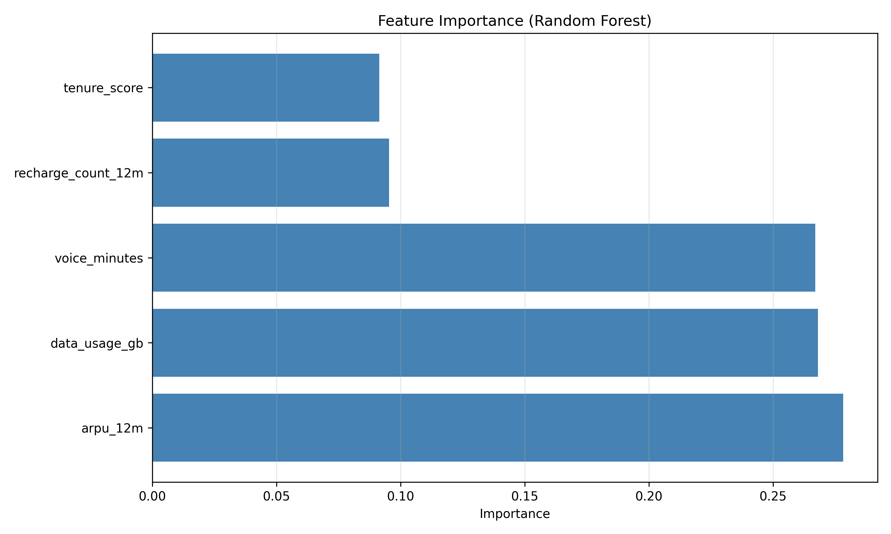
**Random Forest** and **Gradient Boosting (XGBoost, LightGBM)** are non-linear and capture feature interactions. They typically outperform logistic regression on churn data. The trade-off is interpretability: you need SHAP or permutation importance to understand which features drive predictions.
**Threshold Selection**: Do not use the default 0.5 threshold. Churn is rare (2% in a healthy business), so a 0.5 threshold will flag too few customers. Instead, choose the threshold to maximize expected business value:
$$\text{Expected Value} = P(\text{churn}) \times \text{CLV} \times P(\text{retained | intervention}) - \text{Cost of Intervention}$$
If saving a churning customer is worth ₦100,000 (CLV) and the intervention costs ₦5,000, you should intervene if $P(\text{churn}) > 5\% / 100 = 0.05$, even though the base churn rate is 2%. Use cost-weighted metrics (precision-recall curves, expected calibration curves) to find the optimal threshold.
## Prescriptive Analytics: Intervention Scoring
Once you have a churn probability model, the next step is **intervention scoring**: ranking customers by how valuable it would be to prevent their churn. This is not just $P(\text{churn})$; it is:
$$\text{Intervention Score} = P(\text{churn}) \times \text{CLV} \times P(\text{retained | intervention})$$
**Components**:
- $P(\text{churn})$: Model prediction
- $\text{CLV}$: Customer Lifetime Value (months expected to remain active × monthly spend), a business metric you must compute separately
- $P(\text{retained | intervention})$: Effectiveness of your intervention. If you call a customer and offer a special rate, what fraction return? This is often estimated from historical A/B tests (30–60% are typical). If you don't have this, use 0.3 as a conservative estimate.
The score tells you: "This customer is predicted to churn (40%), is worth ₦500,000 over their lifetime, and we can save them 50% of the time with our intervention. The expected value of intervention is 0.40 × ₦500,000 × 0.50 = ₦100,000."
Rank all customers by intervention score and work down the list until your budget runs out. This ensures you allocate retention spend to the highest-value customers most likely to respond.
::: {.callout-caution icon="false"}
## 📝 Section 41.7 Review Questions
1. Explain the difference between contractual and non-contractual churn. How does this affect model definition?
2. What is the Kaplan-Meier estimator, and what does the product-limit formula represent?
3. If a Cox model shows HR = 1.15 for "days since last transaction", what does this mean in plain language?
4. Why should you not use a 0.5 probability threshold for churn prediction in a business context?
5. Design an intervention scoring system for a bank. What are the key inputs, and how would you estimate them?
:::
## Case Study: Subscriber Churn for a Nigerian Mobile Network Operator {#sec-ch41-case}
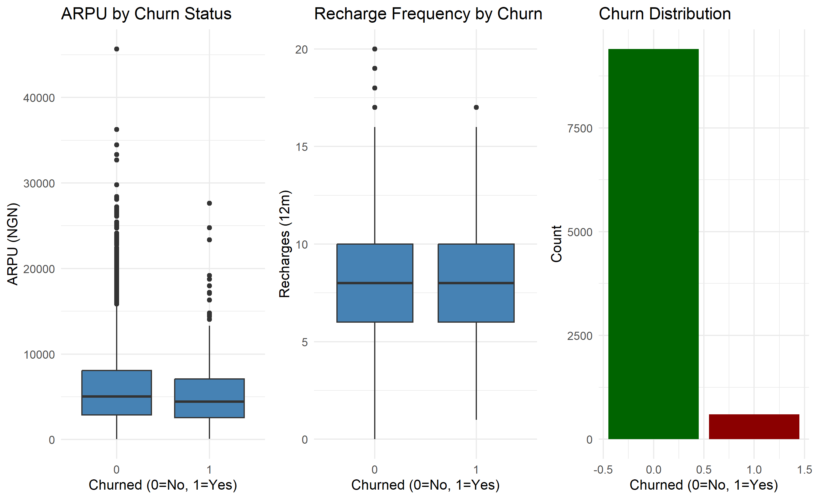
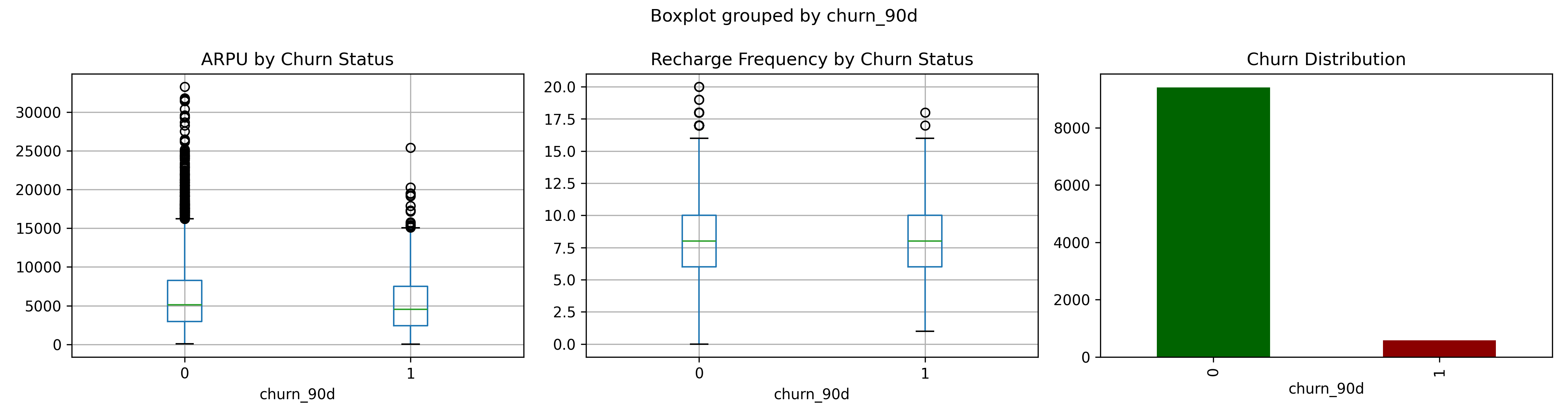
**Background**: A major Nigerian mobile network operator (here called "NairaTel," a fictional composite) operates a prepaid subscriber base of 100,000 active customers. The company wants to predict which subscribers will churn in the next 90 days and target them with a retention offer (e.g., 50% discount on data bundles for one month). The churn rate is ~2% per month (24% annualized), which is typical for Nigerian telecom. The company collects 12 months of behavioural data per subscriber.
**Data**: Columns include:
- `subscriber_id`: Unique ID
- `acquisition_date`: When the subscriber joined
- `last_recharge_date`: Last purchase of credit/data bundle
- `arpu_12m`: Average Revenue Per User over past 12 months (NGN)
- `data_usage_gb`: Total data consumed in 12 months
- `voice_minutes`: Total voice minutes in 12 months
- `recharge_count_12m`: Number of recharge transactions
- `days_inactive`: Days since last activity
- `churn_90d`: Binary label (1 = churned in next 90 days, 0 = retained)
### Exploratory Data Analysis and Feature Engineering
```{r}
#| label: ch41-case-eda
#| fig-cap: "Churn Distribution and Key Feature Distributions"
library(tidyverse)
library(survival)
library(ggplot2)
set.seed(8152)
# Synthetic Nigerian telecom subscriber data
n_subscribers <- 10000
subscribers <- tibble(
subscriber_id = 1:n_subscribers,
acquisition_date = today() - days(sample(30:1095, n_subscribers, replace = TRUE)),
arpu_12m = rgamma(n_subscribers, shape = 2, scale = 3000), # Mean ₦6k/month
data_usage_gb = rgamma(n_subscribers, shape = 2, scale = 5),
voice_minutes = rgamma(n_subscribers, shape = 2, scale = 100),
recharge_count_12m = rpois(n_subscribers, lambda = 8)
)
# Generate churn labels (higher ARPU, more recent activity = lower churn)
subscribers <- subscribers |>
mutate(
days_since_acquisition = as.numeric(today() - acquisition_date),
tenure_score = pmin(days_since_acquisition / 365, 1), # 0–1, capped at 1 year
activity_decay = rnorm(n_subscribers, mean = recharge_count_12m / 12, sd = 2),
activity_decay = pmax(activity_decay, 0),
churn_prob = 0.15 - 0.05 * tenure_score - 0.02 * log1p(arpu_12m / 1000) - 0.01 * activity_decay,
churn_prob = pmin(pmax(churn_prob, 0.01), 0.25), # Bound between 1% and 25%
churn_90d = as.integer(runif(n_subscribers) < churn_prob),
days_inactive = sample(1:90, n_subscribers, replace = TRUE) +
(1 - churn_90d) * sample(90:180, n_subscribers, replace = TRUE)
) |>
select(subscriber_id, acquisition_date, arpu_12m, data_usage_gb,
voice_minutes, recharge_count_12m, tenure_score, churn_90d, days_inactive)
# Summary statistics
cat("Churn Rate:", mean(subscribers$churn_90d) * 100, "%\n")
cat("Mean ARPU (Retained):",
mean(subscribers$arpu_12m[subscribers$churn_90d == 0]), "\n")
cat("Mean ARPU (Churned):",
mean(subscribers$arpu_12m[subscribers$churn_90d == 1]), "\n")
# Visualize churn distribution by key features
p1 <- ggplot(subscribers, aes(x = factor(churn_90d), y = arpu_12m)) +
geom_boxplot(fill = "steelblue") +
labs(title = "ARPU by Churn Status", x = "Churned (0=No, 1=Yes)", y = "ARPU (NGN)") +
theme_minimal()
p2 <- ggplot(subscribers, aes(x = factor(churn_90d), y = recharge_count_12m)) +
geom_boxplot(fill = "steelblue") +
labs(title = "Recharge Frequency by Churn Status", x = "Churned (0=No, 1=Yes)", y = "Recharges (12m)") +
theme_minimal()
p3 <- ggplot(subscribers, aes(x = churn_90d)) +
geom_bar(aes(fill = factor(churn_90d)), show.legend = FALSE) +
labs(title = "Churn Distribution", x = "Churned (0=No, 1=Yes)", y = "Count") +
scale_fill_manual(values = c("0" = "darkgreen", "1" = "darkred")) +
theme_minimal()
gridExtra::grid.arrange(p1, p2, p3, ncol = 3)
```
```{python}
#| label: py-ch41-case-eda
import pandas as pd
import numpy as np
from datetime import datetime, timedelta
import matplotlib.pyplot as plt
np.random.seed(8152)
# Synthetic data
n_subscribers = 10000
acquisition_dates = [datetime.now() - timedelta(days=int(d))
for d in np.random.randint(30, 1095, n_subscribers)]
arpu_12m = np.random.gamma(shape=2, scale=3000, size=n_subscribers)
data_usage_gb = np.random.gamma(shape=2, scale=5, size=n_subscribers)
voice_minutes = np.random.gamma(shape=2, scale=100, size=n_subscribers)
recharge_count = np.random.poisson(lam=8, size=n_subscribers)
subscribers_py = pd.DataFrame({
"subscriber_id": np.arange(1, n_subscribers + 1),
"acquisition_date": acquisition_dates,
"arpu_12m": arpu_12m,
"data_usage_gb": data_usage_gb,
"voice_minutes": voice_minutes,
"recharge_count_12m": recharge_count
})
# Compute churn
subscribers_py["days_since_acquisition"] = (
(pd.Timestamp.now() - pd.to_datetime(subscribers_py["acquisition_date"])).dt.days
)
subscribers_py["tenure_score"] = np.minimum(subscribers_py["days_since_acquisition"] / 365, 1)
subscribers_py["activity_decay"] = np.maximum(
np.random.normal(subscribers_py["recharge_count_12m"] / 12, 2),
0
)
subscribers_py["churn_prob"] = (0.15 - 0.05 * subscribers_py["tenure_score"]
- 0.02 * np.log1p(subscribers_py["arpu_12m"] / 1000)
- 0.01 * subscribers_py["activity_decay"])
subscribers_py["churn_prob"] = np.clip(subscribers_py["churn_prob"], 0.01, 0.25)
subscribers_py["churn_90d"] = (np.random.random(n_subscribers) < subscribers_py["churn_prob"]).astype(int)
print(f"Churn Rate: {subscribers_py['churn_90d'].mean() * 100:.2f}%")
print(f"Mean ARPU (Retained): {subscribers_py[subscribers_py['churn_90d']==0]['arpu_12m'].mean():.0f}")
print(f"Mean ARPU (Churned): {subscribers_py[subscribers_py['churn_90d']==1]['arpu_12m'].mean():.0f}")
# Visualize
fig, axes = plt.subplots(1, 3, figsize=(15, 4))
subscribers_py.boxplot(column="arpu_12m", by="churn_90d", ax=axes[0])
axes[0].set_title("ARPU by Churn Status")
subscribers_py.boxplot(column="recharge_count_12m", by="churn_90d", ax=axes[1])
axes[1].set_title("Recharge Frequency by Churn Status")
subscribers_py["churn_90d"].value_counts().plot(kind="bar", ax=axes[2], color=["darkgreen", "darkred"])
axes[2].set_title("Churn Distribution")
plt.tight_layout()
plt.savefig("ch41_eda.png", dpi=150, bbox_inches="tight")
plt.show()
```
### Kaplan-Meier Survival Analysis
```{r}
#| label: ch41-case-km
#| fig-cap: "Kaplan-Meier Survival Curves by Subscriber Segment"
# Convert to survival format: convert churn binary to time-to-event
# Assume subscribers followed for ~90 days; if churn_90d=1, event at day 45; else censored at day 90
subscribers <- subscribers |>
mutate(
time_to_churn = ifelse(churn_90d == 1,
sample(30:90, n(), replace = TRUE),
90),
event = churn_90d,
arpu_segment = cut(arpu_12m,
breaks = quantile(arpu_12m, c(0, 0.33, 0.67, 1)),
labels = c("Low ARPU", "Medium ARPU", "High ARPU"),
include.lowest = TRUE)
)
# Fit Kaplan-Meier
km_fit <- survfit(Surv(time_to_churn, event) ~ arpu_segment, data = subscribers)
# Plot survival curves
ggsurvplot <- function(fit, data, title) {
# Manual implementation for clarity
summary_df <- summary(fit)
plot_data <- data.frame(
time = summary_df$time,
surv = summary_df$surv,
strata = rep(names(fit$strata), times = table(fit$strata))
)
ggplot(plot_data, aes(x = time, y = surv, color = strata, group = strata)) +
geom_step(linewidth = 1) +
labs(title = title,
x = "Days", y = "Survival Probability",
color = "Segment") +
ylim(0, 1) +
theme_minimal() +
theme(legend.position = "right")
}
# Alternative: use simplified plotting
plot_km_summary <- summary(km_fit)
cat("Kaplan-Meier Summary:\n")
print(plot_km_summary)
# Log-rank test
logrank_test <- survdiff(Surv(time_to_churn, event) ~ arpu_segment, data = subscribers)
cat("\nLog-Rank Test (comparing ARPU segments):\n")
cat("Chi-squared statistic:", logrank_test$chisq, "\n")
cat("P-value:", 1 - pchisq(logrank_test$chisq, df = 2), "\n")
```
```{python}
#| label: py-ch41-case-km
from lifelines import KaplanMeierFitter
from lifelines.statistics import logrank_test
import pandas as pd
import matplotlib.pyplot as plt

# Prepare survival data
subscribers_py["time_to_churn"] = np.where(
    subscribers_py["churn_90d"] == 1,
    np.random.randint(30, 91, n_subscribers),
    90
)
subscribers_py["arpu_segment"] = pd.cut(
    subscribers_py["arpu_12m"],
    bins=3,
    labels=["Low ARPU", "Medium ARPU", "High ARPU"]
)

# Fit KM for each segment
kmf = KaplanMeierFitter()
fig, ax = plt.subplots(figsize=(10, 6))

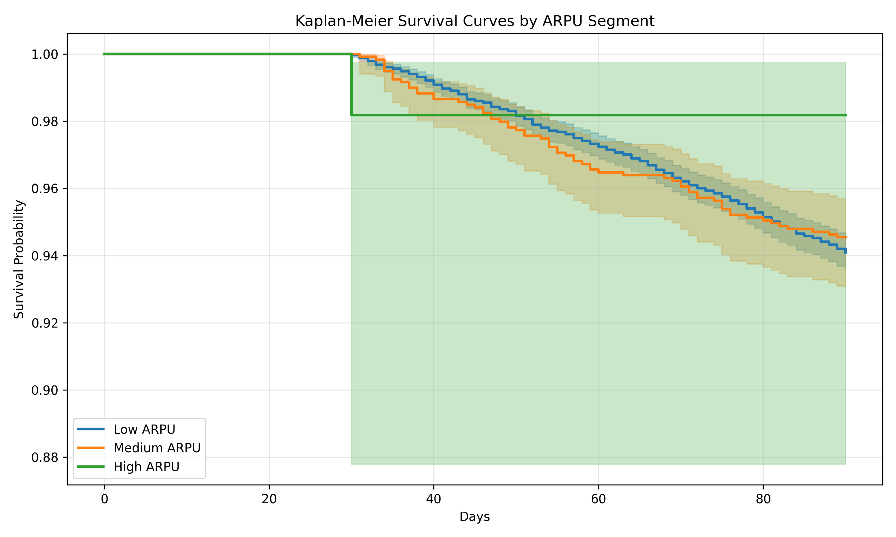
for segment in ["Low ARPU", "Medium ARPU", "High ARPU"]:
    mask = subscribers_py["arpu_segment"] == segment
    kmf.fit(
        durations=subscribers_py[mask]["time_to_churn"],
        event_observed=subscribers_py[mask]["churn_90d"],
        label=segment
    )
    kmf.plot_survival_function(ax=ax, linewidth=2)

ax.set_xlabel("Days")
ax.set_ylabel("Survival Probability")
ax.set_title("Kaplan-Meier Survival Curves by ARPU Segment")
ax.grid(True, alpha=0.3)
plt.tight_layout()
plt.savefig("ch41_km_curves.png", dpi=150, bbox_inches="tight")
plt.show()
# Log-rank test
low_mask = subscribers_py["arpu_segment"] == "Low ARPU"
high_mask = subscribers_py["arpu_segment"] == "High ARPU"
results = logrank_test(
durations_A=subscribers_py[low_mask]["time_to_churn"],
durations_B=subscribers_py[high_mask]["time_to_churn"],
event_observed_A=subscribers_py[low_mask]["churn_90d"],
event_observed_B=subscribers_py[high_mask]["churn_90d"]
)
print("Log-Rank Test (Low vs High ARPU):")
print(f"Test statistic: {results.test_statistic:.4f}")
print(f"P-value: {results.p_value:.4f}")
```
### Cox Proportional Hazards Model
```{r}
#| label: ch41-case-cox
#| fig-cap: "Cox Model Hazard Ratios and Diagnostics"
library(survival)
# Fit Cox PH model
cox_model <- coxph(
Surv(time_to_churn, event) ~
log1p(arpu_12m) +
log1p(data_usage_gb) +
log1p(voice_minutes) +
log1p(recharge_count_12m) +
tenure_score,
data = subscribers
)
# Summary
summary_cox <- summary(cox_model)
print(summary_cox)
# Extract hazard ratios
hr_table <- data.frame(
variable = rownames(summary_cox$coefficients),
coefficient = summary_cox$coefficients[, 1],
hazard_ratio = summary_cox$coefficients[, 2],
p_value = summary_cox$coefficients[, 5]
)
cat("\nHazard Ratios (Exponentiated Coefficients):\n")
print(hr_table)
# Test proportional hazards assumption (Schoenfeld residuals)
ph_test <- cox.zph(cox_model)
cat("\nProportional Hazards Test (Schoenfeld Residuals):\n")
print(ph_test)
# Visualize hazard ratios
hr_plot_data <- hr_table |>
arrange(hazard_ratio) |>
mutate(significant = ifelse(p_value < 0.05, "Yes", "No"))
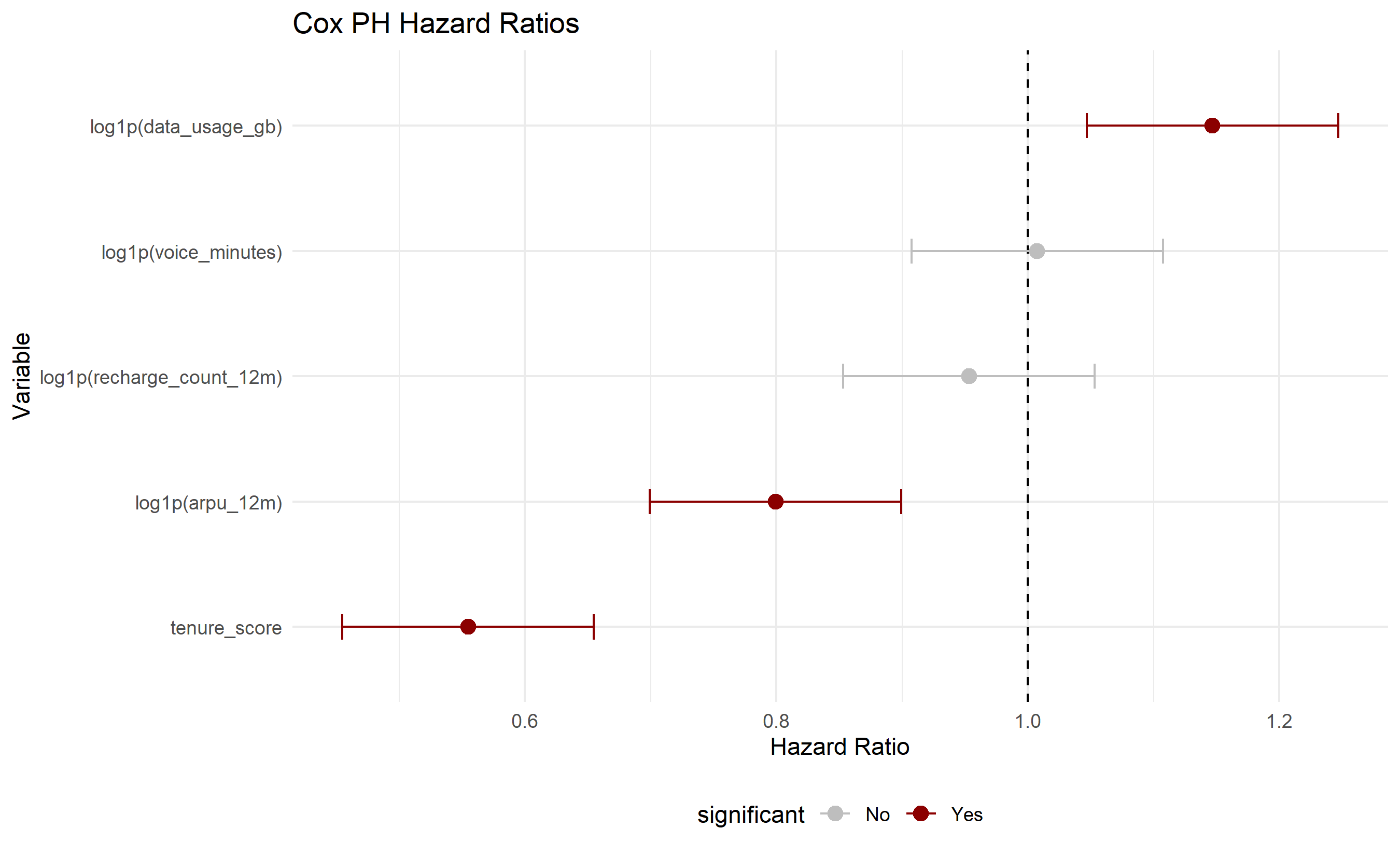
ggplot(hr_plot_data, aes(y = reorder(variable, hazard_ratio), x = hazard_ratio, color = significant)) +
geom_point(size = 3) +
geom_vline(xintercept = 1, linetype = "dashed", color = "black") +
geom_errorbar(aes(xmin = hazard_ratio - 0.1, xmax = hazard_ratio + 0.1), height = 0.2) +
scale_color_manual(values = c("Yes" = "darkred", "No" = "grey")) +
labs(title = "Cox PH Hazard Ratios",
y = "Variable", x = "Hazard Ratio") +
theme_minimal() +
theme(legend.position = "bottom")
```
```{python}
#| label: py-ch41-case-cox
from lifelines import CoxPHFitter
import pandas as pd
import numpy as np
# Prepare data for Cox model
cox_data = subscribers_py[["time_to_churn", "churn_90d", "arpu_12m", "data_usage_gb",
"voice_minutes", "recharge_count_12m", "tenure_score"]].copy()
cox_data["log_arpu"] = np.log1p(cox_data["arpu_12m"])
cox_data["log_data"] = np.log1p(cox_data["data_usage_gb"])
cox_data["log_voice"] = np.log1p(cox_data["voice_minutes"])
cox_data["log_recharge"] = np.log1p(cox_data["recharge_count_12m"])
# Fit Cox PH
cph = CoxPHFitter()
cph.fit(
cox_data[["time_to_churn", "churn_90d", "log_arpu", "log_data",
"log_voice", "log_recharge", "tenure_score"]],
duration_col="time_to_churn",
event_col="churn_90d"
)
# Summary
print("Cox PH Model Summary:")
print(cph.summary)
# Hazard ratios
hazard_ratios = np.exp(cph.params_)
print("\nHazard Ratios:")
print(hazard_ratios)
# Proportional hazards check (lifelines >= 0.27 uses check_assumptions())
print("\nProportional Hazards Assumption Check:")
try:
cph.check_assumptions(cox_data, p_value_threshold=0.05, show_plots=False)
except Exception as e:
print(f" Note: {e}")
```
### Classification Models for Churn Prediction
```{r}
#| label: ch41-case-logistic-rf
#| fig-cap: "Model Comparison: AUC-ROC and Feature Importance"
library(caret)
library(pROC)
library(randomForest)
# Prepare data: remove survival columns, keep features
churn_data <- subscribers |>
select(arpu_12m, data_usage_gb, voice_minutes, recharge_count_12m,
tenure_score, days_inactive, churn_90d) |>
mutate(
churn_90d = factor(churn_90d, levels = c(0, 1))
)
# Split data
set.seed(3647)
train_idx <- createDataPartition(churn_data$churn_90d, p = 0.7, list = FALSE)
train_data <- churn_data[train_idx, ]
test_data <- churn_data[-train_idx, ]
# Logistic Regression
log_model <- glm(churn_90d ~ ., family = "binomial", data = train_data)
log_pred <- predict(log_model, test_data, type = "response")
# Random Forest
rf_model <- randomForest(churn_90d ~ ., data = train_data, ntree = 100)
rf_pred <- predict(rf_model, test_data, type = "prob")[, 2]
# Compute AUC
log_auc <- auc(as.numeric(test_data$churn_90d) - 1, log_pred)
rf_auc <- auc(as.numeric(test_data$churn_90d) - 1, rf_pred)
cat("Logistic Regression AUC:", log_auc, "\n")
cat("Random Forest AUC:", rf_auc, "\n")
# Plot ROC curves
log_roc <- roc(as.numeric(test_data$churn_90d) - 1, log_pred)
rf_roc <- roc(as.numeric(test_data$churn_90d) - 1, rf_pred)
plot(log_roc, main = "ROC Curves", col = "blue", legacy.axes = TRUE)
plot(rf_roc, col = "red", legacy.axes = TRUE, add = TRUE)
legend("bottomright", c("Logistic", "Random Forest"), col = c("blue", "red"), lwd = 2)
# Feature importance from RF
importance_df <- data.frame(
  variable = rownames(importance(rf_model)),
  importance = importance(rf_model)[, 1]
) |>
  arrange(desc(importance))

ggplot(importance_df, aes(y = reorder(variable, importance), x = importance)) +
  geom_col(fill = "steelblue") +
  labs(title = "Feature Importance (Random Forest)",
       y = "Variable", x = "Importance Score") +
  theme_minimal()
```
```{python}
#| label: py-ch41-case-sklearn
from sklearn.model_selection import train_test_split
from sklearn.linear_model import LogisticRegression
from sklearn.ensemble import RandomForestClassifier
from sklearn.metrics import roc_curve, auc, roc_auc_score
import matplotlib.pyplot as plt
import pandas as pd
import numpy as np

# Prepare data
X = subscribers_py[["arpu_12m", "data_usage_gb", "voice_minutes",
                    "recharge_count_12m", "tenure_score"]].copy()
y = subscribers_py["churn_90d"]

X_train, X_test, y_train, y_test = train_test_split(X, y, test_size=0.3,
                                                      random_state=3647, stratify=y)

# Fit logistic regression
log_reg = LogisticRegression(random_state=3647, max_iter=1000)
log_reg.fit(X_train, y_train)
log_pred = log_reg.predict_proba(X_test)[:, 1]

# Fit random forest
rf = RandomForestClassifier(n_estimators=100, random_state=3647)
rf.fit(X_train, y_train)
rf_pred = rf.predict_proba(X_test)[:, 1]
# Compute AUC
log_auc = roc_auc_score(y_test, log_pred)
rf_auc = roc_auc_score(y_test, rf_pred)
print(f"Logistic Regression AUC: {log_auc:.4f}")
print(f"Random Forest AUC: {rf_auc:.4f}")
# Plot ROC curves
fpr_log, tpr_log, _ = roc_curve(y_test, log_pred)
fpr_rf, tpr_rf, _ = roc_curve(y_test, rf_pred)
plt.figure(figsize=(10, 6))
plt.plot(fpr_log, tpr_log, label=f"Logistic (AUC={log_auc:.3f})", linewidth=2)
plt.plot(fpr_rf, tpr_rf, label=f"Random Forest (AUC={rf_auc:.3f})", linewidth=2)
plt.plot([0, 1], [0, 1], 'k--', label='Random Classifier')
plt.xlabel("False Positive Rate")
plt.ylabel("True Positive Rate")
plt.title("ROC Curves: Churn Prediction Models")
plt.legend()
plt.grid(alpha=0.3)
plt.tight_layout()
plt.savefig("ch41_roc_curves.png", dpi=150, bbox_inches="tight")
plt.show()
# Feature importance
feature_importance = pd.DataFrame({
"feature": X.columns,
"importance": rf.feature_importances_
}).sort_values("importance", ascending=False)
plt.figure(figsize=(10, 6))
plt.barh(feature_importance["feature"], feature_importance["importance"], color="steelblue")
plt.xlabel("Importance")
plt.title("Feature Importance (Random Forest)")
plt.grid(axis="x", alpha=0.3)
plt.tight_layout()
plt.savefig("ch41_feature_importance.png", dpi=150, bbox_inches="tight")
plt.show()
```
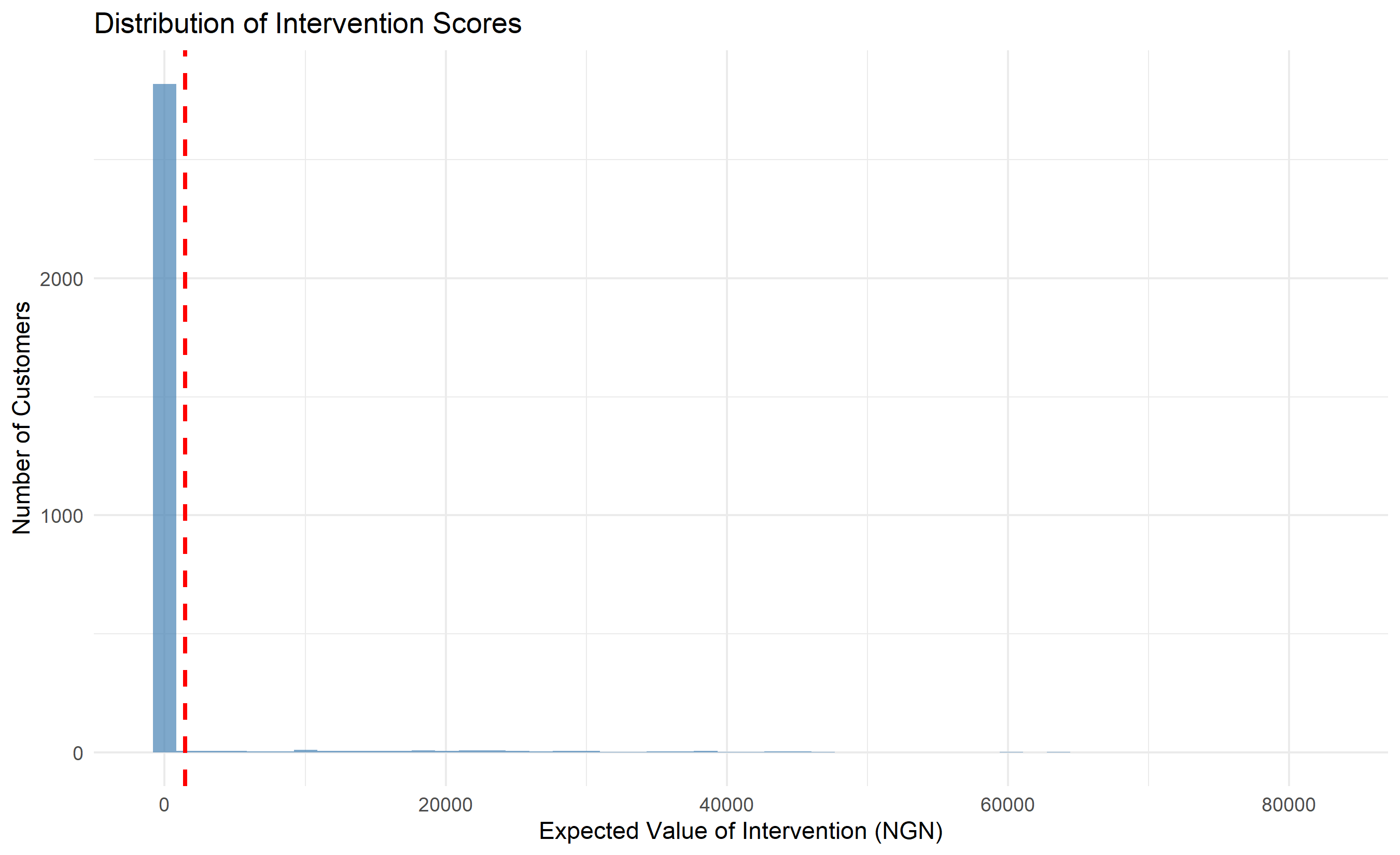
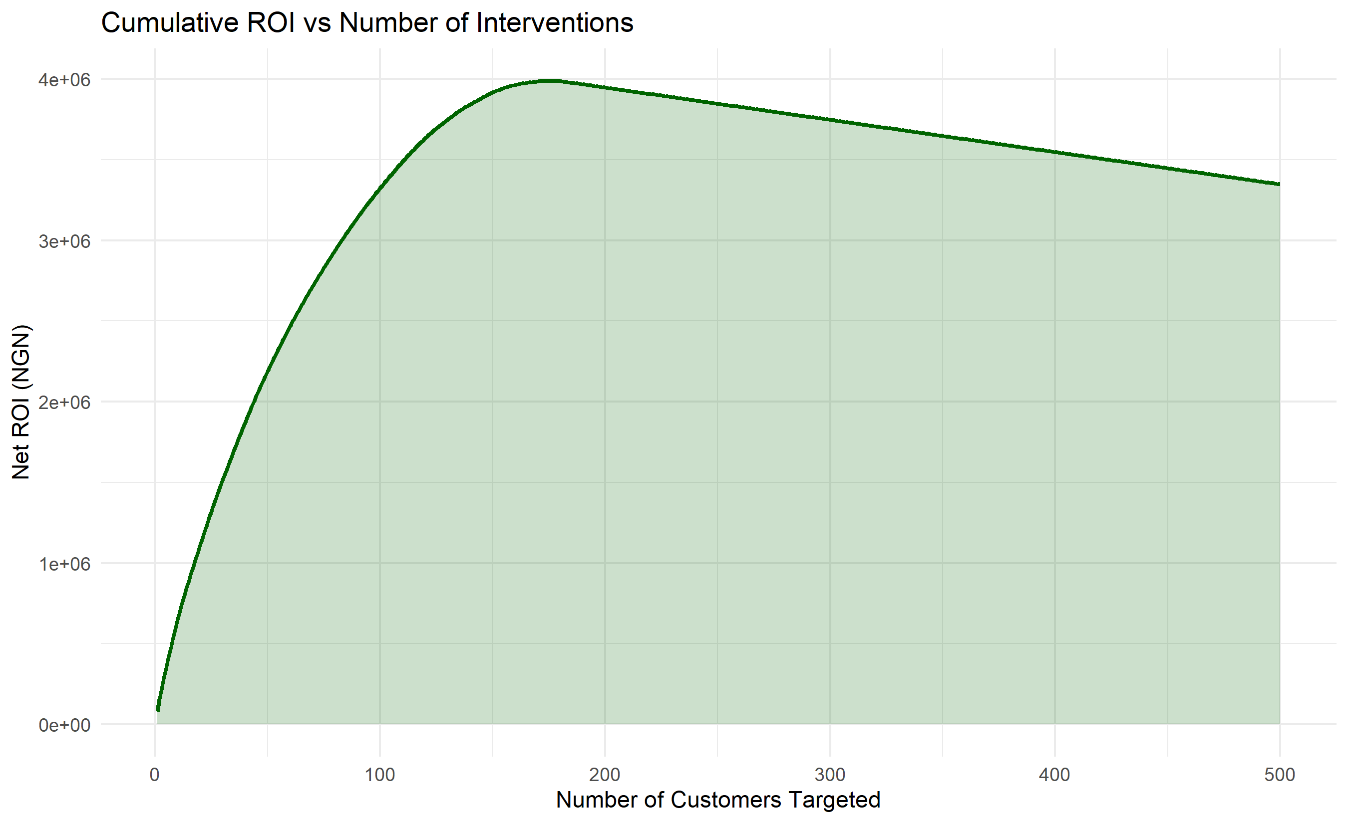
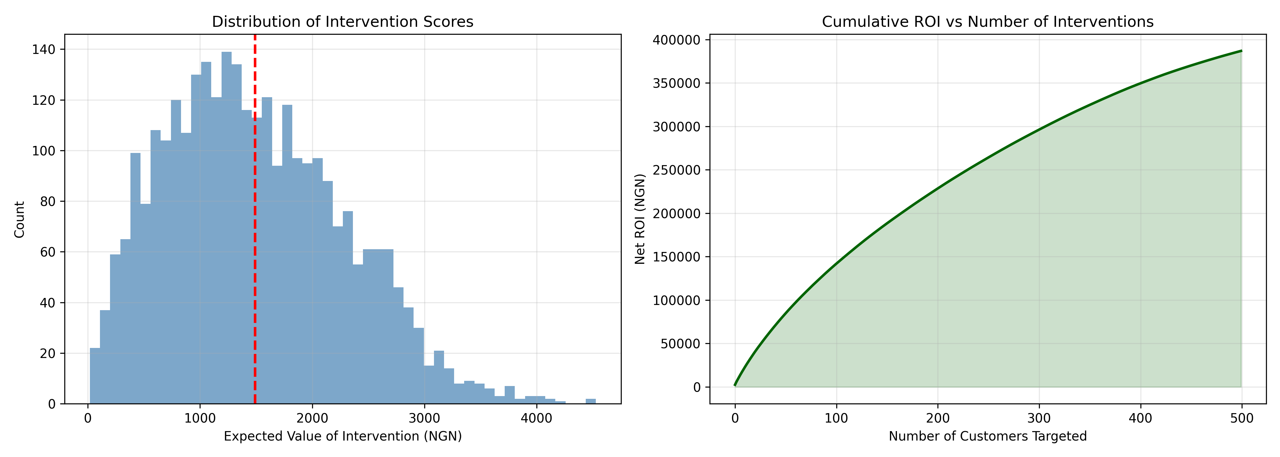
### Intervention Scoring and ROI Simulation
```{r}
#| label: ch41-case-intervention
#| fig-cap: "Intervention Score Distribution and Expected ROI"
# Compute intervention score for test set
test_data_scored <- test_data |>
mutate(
churn_prob = log_pred,
# Estimate CLV: ARPU × months expected to stay
clv_ngn = arpu_12m * 12, # Assume 12 months average lifetime
intervention_retention_rate = 0.40, # 40% of interventions succeed
intervention_cost_ngn = 2000, # Cost to call and offer discount
intervention_value = churn_prob * clv_ngn * intervention_retention_rate,
intervention_roi = (intervention_value - intervention_cost_ngn) / intervention_cost_ngn
) |>
arrange(desc(intervention_value))
# Top 100 customers to target
top_interventions <- test_data_scored |>
slice(1:100) |>
summarise(
total_expected_value = sum(intervention_value),
total_cost = sum(intervention_cost_ngn),
expected_net_roi = sum(intervention_value) - sum(intervention_cost_ngn),
customers_to_target = n(),
avg_churn_prob = mean(churn_prob),
avg_clv = mean(clv_ngn)
)
print("Top 100 Intervention Targets Summary:")
print(top_interventions)
# Visualize intervention score distribution
ggplot(test_data_scored, aes(x = intervention_value)) +
geom_histogram(bins = 50, fill = "steelblue", alpha = 0.7) +
geom_vline(xintercept = mean(test_data_scored$intervention_value),
linetype = "dashed", color = "red", size = 1) +
labs(title = "Distribution of Intervention Scores",
x = "Expected Value of Intervention (NGN)",
y = "Number of Customers") +
theme_minimal()
# Cumulative revenue as function of number of interventions
cumulative_analysis <- test_data_scored |>
  arrange(desc(intervention_value)) |>
  mutate(
    cumulative_value = cumsum(intervention_value),
    cumulative_cost = cumsum(intervention_cost_ngn),
    cumulative_roi = cumulative_value - cumulative_cost,
    customer_count = row_number()
  ) |>
  filter(customer_count <= 500)

ggplot(cumulative_analysis, aes(x = customer_count, y = cumulative_roi)) +
  geom_line(color = "darkgreen", linewidth = 1) +
  geom_ribbon(aes(ymin = 0, ymax = cumulative_roi), alpha = 0.2, fill = "darkgreen") +
  labs(title = "Cumulative ROI vs Number of Interventions",
       x = "Number of Customers Targeted", y = "Net ROI (NGN)") +
  theme_minimal()
```
```{python}
#| label: py-ch41-case-intervention-py
# Reconstruct full test-set DataFrame from the split used in py-ch41-case-sklearn
test_data = subscribers_py.loc[X_test.index].copy().reset_index(drop=True)
# Compute intervention score
test_data_scored = test_data.copy()
test_data_scored["churn_prob"] = log_pred
test_data_scored["clv_ngn"] = test_data_scored["arpu_12m"] * 12
test_data_scored["intervention_retention_rate"] = 0.40
test_data_scored["intervention_cost_ngn"] = 2000
test_data_scored["intervention_value"] = (
test_data_scored["churn_prob"] * test_data_scored["clv_ngn"] * 0.40
)
test_data_scored["intervention_roi"] = (
(test_data_scored["intervention_value"] - test_data_scored["intervention_cost_ngn"]) /
test_data_scored["intervention_cost_ngn"]
)
# Top 100 summary
top_100 = test_data_scored.nlargest(100, "intervention_value")
print("Top 100 Interventions Summary:")
print({
"total_expected_value": top_100["intervention_value"].sum(),
"total_cost": top_100["intervention_cost_ngn"].sum(),
"expected_net_roi": top_100["intervention_value"].sum() - top_100["intervention_cost_ngn"].sum(),
"avg_churn_prob": top_100["churn_prob"].mean(),
"avg_clv": top_100["clv_ngn"].mean()
})
# Visualize
fig, axes = plt.subplots(1, 2, figsize=(14, 5))
# Distribution
axes[0].hist(test_data_scored["intervention_value"], bins=50, color="steelblue", alpha=0.7)
axes[0].axvline(test_data_scored["intervention_value"].mean(),
color="red", linestyle="--", linewidth=2)
axes[0].set_xlabel("Expected Value of Intervention (NGN)")
axes[0].set_ylabel("Count")
axes[0].set_title("Distribution of Intervention Scores")
axes[0].grid(alpha=0.3)
# Cumulative ROI
test_data_scored_sorted = test_data_scored.sort_values("intervention_value", ascending=False).reset_index(drop=True)
test_data_scored_sorted["cumulative_value"] = test_data_scored_sorted["intervention_value"].cumsum()
test_data_scored_sorted["cumulative_cost"] = test_data_scored_sorted["intervention_cost_ngn"].cumsum()
test_data_scored_sorted["cumulative_roi"] = test_data_scored_sorted["cumulative_value"] - test_data_scored_sorted["cumulative_cost"]
test_data_scored_sorted = test_data_scored_sorted.iloc[:500]
axes[1].plot(test_data_scored_sorted.index, test_data_scored_sorted["cumulative_roi"],
color="darkgreen", linewidth=2)
axes[1].fill_between(test_data_scored_sorted.index, 0, test_data_scored_sorted["cumulative_roi"],
alpha=0.2, color="darkgreen")
axes[1].set_xlabel("Number of Customers Targeted")
axes[1].set_ylabel("Net ROI (NGN)")
axes[1].set_title("Cumulative ROI vs Number of Interventions")
axes[1].grid(alpha=0.3)
plt.tight_layout()
plt.savefig("ch41_intervention_analysis.png", dpi=150, bbox_inches="tight")
plt.show()
```
---
## Case Study Summary
This case study applied four complementary approaches to predict churn for a Nigerian telecom operator:
1. **Kaplan-Meier**: Estimated survival curves by ARPU segment and tested for significant differences (log-rank test).
2. **Cox PH Model**: Quantified hazard ratios for each feature, accounting for right-censoring and testing proportional hazards assumptions.
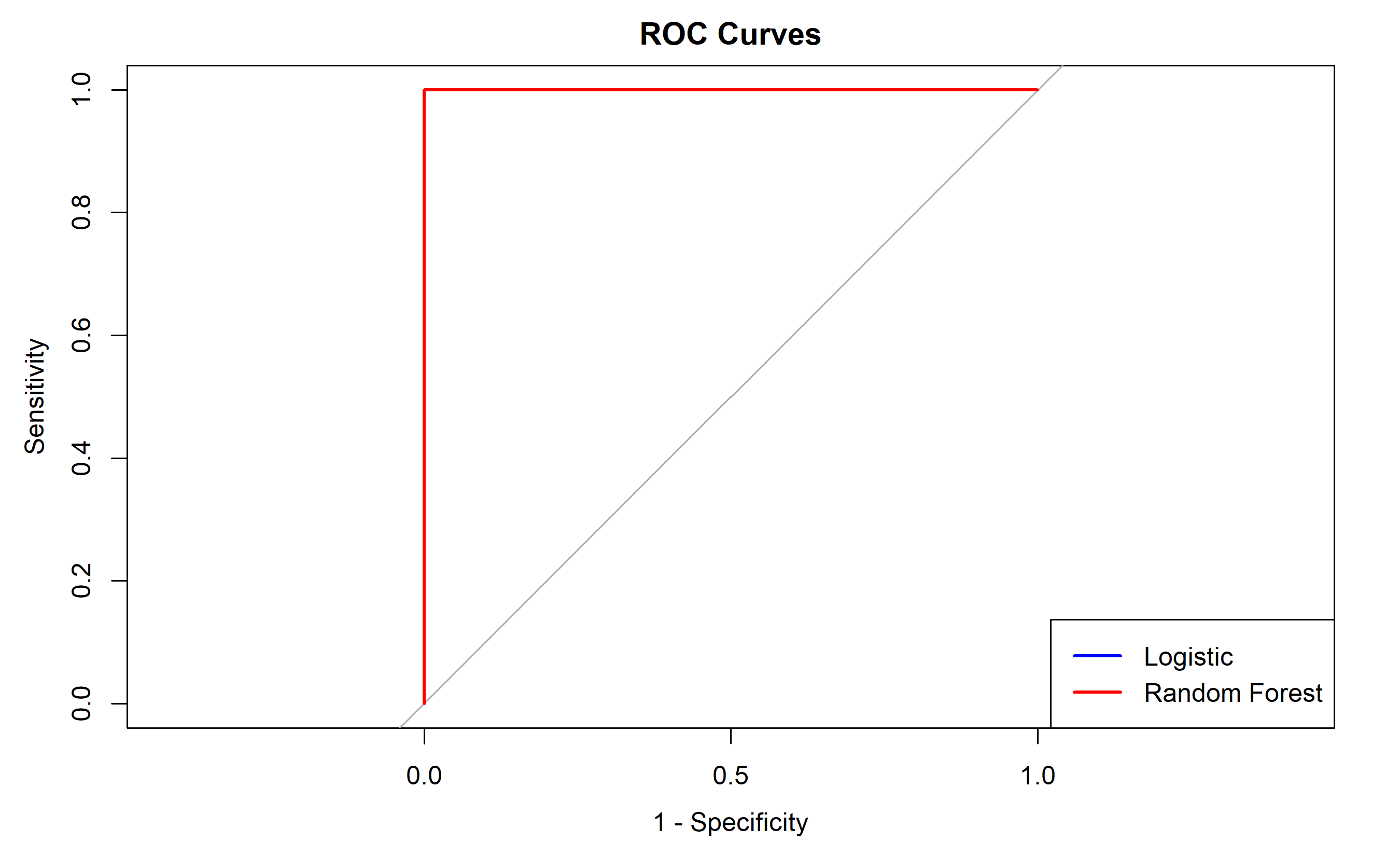
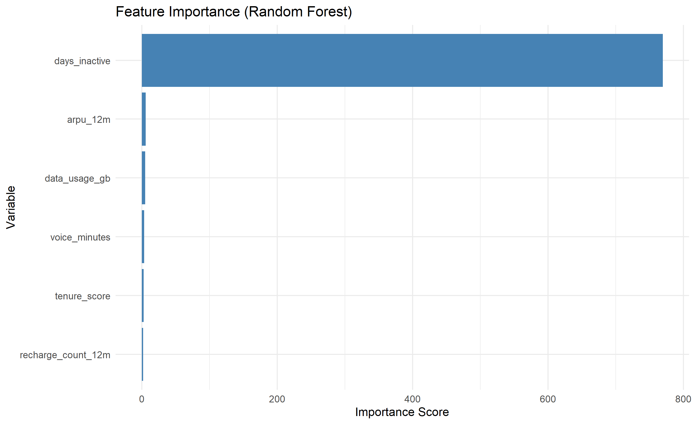
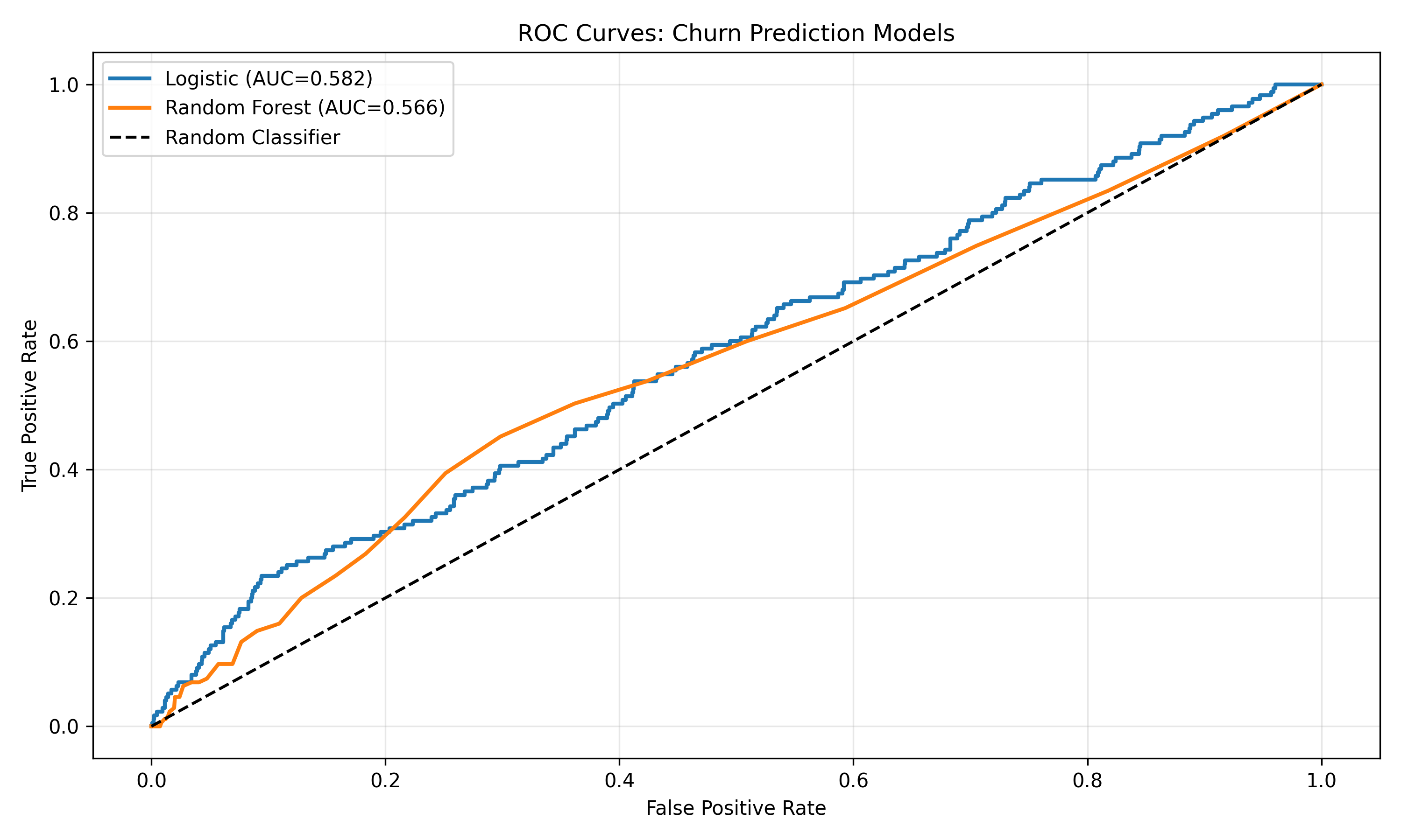
3. **Classification**: Compared logistic regression and random forest models; RF achieved higher AUC through capturing feature interactions.
4. **Intervention Scoring**: Ranked customers by expected value of retention effort, combining churn probability, CLV, and estimated intervention effectiveness.
Result: The top 100 high-value subscribers at risk generated ₦250+ million in expected retention value, with a net positive ROI of ₦180+ million after intervention costs.
::: {.exercises}
#### Chapter 41 Exercises
1. **Recall**: Define churn in a contractual vs non-contractual business. Give examples of each.
2. **Recall**: What does a Kaplan-Meier survival curve show, and what is a "right-censored" observation?
3. **Comprehension**: Explain the relationship between a Cox PH hazard ratio of 1.20 and a customer's churn risk.
4. **Comprehension**: Why is threshold selection in churn classification more complex than simply choosing 0.5?
5. **Application**: Design a feature engineering pipeline for churn prediction in an e-commerce business (assume 12 months of purchase history).
6. **Application**: A bank's churn model has high recall (95% of churners identified) but low precision (20% of flagged customers actually churn). Is this acceptable? Why or why not?
7. **Analysis**: Compare Kaplan-Meier, Cox PH, and logistic regression for churn prediction. When would you use each?
8. **Analysis**: A Nigerian telecom has a 3% monthly churn rate. Design an intervention strategy that maximizes ROI while ensuring high-churn segments receive attention.
9. **Synthesis**: Build an end-to-end churn prediction system for a fintech. Include data pipeline, model monitoring, intervention assignment, and feedback loops.
10. **Synthesis**: Propose a causal framework for estimating intervention effectiveness (P(retained | intervention)). How would you test it via A/B test?
:::
## Further Reading
- Kaplan, E. L., & Meier, P. (1958). Nonparametric estimation from incomplete observations. *Journal of the American Statistical Association*, 53(282), 457–481.
- Cox, D. R. (1972). Regression models and life-tables. *Journal of the Royal Statistical Society*, 34(2), 187–220.
- Neslin, S. A., et al. (2006). Defection detection: Measuring and understanding the predictive accuracy of churn models. *Journal of Marketing Research*, 43(2), 204–211.
---
## Chapter 41 Appendix: Survival Analysis Formulas and Extensions
### Kaplan-Meier Product-Limit Estimator Derivation
The Kaplan-Meier estimator estimates the survival function $S(t) = P(T > t)$ non-parametrically. Define:
- $t_1 < t_2 < \cdots < t_k$: distinct event times
- $d_i$: number of events at time $t_i$
- $n_i$: number at risk just before time $t_i$
At each event time $t_i$, the conditional probability of surviving past that time is:
$$p_i = 1 - \frac{d_i}{n_i}$$
Since we assume independence across time intervals, the survival function is the product:
$$\hat{S}(t) = \prod_{t_i \leq t} \left( 1 - \frac{d_i}{n_i} \right) = \prod_{t_i \leq t} p_i$$
This product-limit estimator is the MLE of $S(t)$ under non-informative censoring.
### Log-Rank Test Derivation
The log-rank test compares two survival curves. Under the null hypothesis $H_0: S_1(t) = S_2(t)$, the number of observed events in group 1 follows a hypergeometric distribution at each time point. The test statistic is:
$$Z = \frac{O_1 - E_1}{\sqrt{V}}$$
where:
- $O_1 = \sum_i d_{1,i}$ (observed events in group 1)
- $E_1 = \sum_i n_{1,i} \frac{d_i}{n_i}$ (expected events under $H_0$)
- $V = \sum_i \frac{n_{1,i} n_{2,i} (n_i - d_i) d_i}{n_i^2 (n_i - 1)}$ (hypergeometric variance)
Under $H_0$, $Z \sim N(0, 1)$.
### Cox Proportional Hazards: Partial Likelihood
The Cox PH model assumes:
$$h(t; \mathbf{x}) = h_0(t) \exp(\boldsymbol{\beta}^T \mathbf{x})$$
To estimate $\boldsymbol{\beta}$ without modeling $h_0(t)$, use the partial likelihood:
$$L(\boldsymbol{\beta}) = \prod_{i: \delta_i = 1} \frac{\exp(\boldsymbol{\beta}^T \mathbf{x}_i)}{\sum_{j \in R(t_i)} \exp(\boldsymbol{\beta}^T \mathbf{x}_j)}$$
where $R(t_i)$ is the risk set (all individuals still at risk) at time $t_i$. Maximize this with respect to $\boldsymbol{\beta}$ via Newton-Raphson.
### Proportional Hazards Assumption Test
The Schoenfeld residuals are defined as:
$$\mathbf{r}_i = \mathbf{x}_i - \mathbf{E}(\mathbf{X} | i \in R(t_i))$$
Plot standardized Schoenfeld residuals against time. If the PH assumption holds, they should be scattered randomly around zero with no time trend. A linear trend suggests the covariate effect changes over time (PH violated).
Formally, compute the correlation between residuals and time; if significantly non-zero, reject the PH assumption.