20  Random Forests, Gradient Boosting, and Ensemble Methods

Note📋 Learning Objectives

By the end of this chapter, you will be able to:

• Understand the wisdom of crowds principle and why ensembles outperform single models
• Explain the bias-variance trade-off and how ensembles reduce variance
• Implement bootstrap aggregation (bagging) from scratch
• Build and tune Random Forests for classification and regression
• Train and deploy Gradient Boosting models (XGBoost, LightGBM)
• Interpret variable importance from ensemble models
• Apply learning curves and early stopping to detect overfitting
• Compare decision trees, Random Forests, and boosted models on the same dataset
• Conduct hyperparameter grid search with cross-validation

20.1 The Wisdom of Crowds: Why Many Weak Models Beat One Strong One

In 1907, the statistician Francis Galton attended a livestock fair in England. Visitors were invited to guess the weight of an ox. About 800 people submitted guesses — farmers, butchers, and curious onlookers. Most individual guesses were wrong. Some were wildly off. But Galton noticed something remarkable: when he calculated the median of all the guesses, the answer was 1,207 pounds. The actual weight of the ox: 1,198 pounds. A crowd of 800 imperfect guessers was collectively more accurate than any single expert.

This is the wisdom of crowds — and it is the central idea behind ensemble learning in machine learning.

Consider a fraud detection model at a Nigerian bank. A single decision tree might be 78% accurate — it makes some correct decisions and some wrong ones. Now suppose you train 500 different decision trees, each on a slightly different random sample of the training data. Each tree makes its own set of mistakes. But — and this is crucial — the mistakes are different for different trees. Tree 47 might misclassify a particular transaction that Tree 203 gets right. Tree 119 might flag a legitimate transaction that Trees 312 and 445 correctly approve. When you let all 500 trees vote, the majority vote is almost always right, because the errors cancel out. The result: a collection of individually weak models combines into a collectively strong one.

This is Random Forest — and it consistently ranks among the most reliable, accurate, and robust models in practical machine learning. Unlike a single decision tree (which can be overly sensitive to the exact training data it saw), a Random Forest is stable. Unlike a deep neural network (which requires enormous datasets and computational resources), a Random Forest trains quickly and works well on datasets of almost any size. It handles missing values, mixed data types, and non-linear relationships gracefully. In a survey of Kaggle competition winners across many years, Random Forest and gradient boosting (its close relative) were the most frequently cited model families.

Ensemble methods combine multiple models — the “weak learners” — to achieve better predictions than any single model could achieve alone. The key theoretical insight: if models make independent errors, averaging their predictions reduces variance without increasing bias.

Note📘 Theory: Why Ensembles Work

Suppose we have B independent estimators \(\hat{f}_1(x), \hat{f}_2(x), \ldots, \hat{f}_B(x)\) of the true function f(x), each with bias β and variance σ².

Single model: - Bias = β - Variance = σ² - Mean Squared Error = β² + σ²

Ensemble (averaging): \[\hat{f}_{ensemble}(x) = \frac{1}{B} \sum_{b=1}^{B} \hat{f}_b(x)\]

• Bias = β (unchanged; if each estimator is biased, the average is too)
• Variance = σ²/B (reduced by factor B!)
• Mean Squared Error = β² + σ²/B

Conclusion: Ensembles reduce variance without increasing bias, provided the base learners are uncorrelated. High correlation among learners means the ensemble variance reduction is minimal.

Tip🔑 Key Formula: Ensemble Variance Reduction

Single model: \(MSE = Bias^2 + Variance\)

Ensemble average (independent errors): \(MSE = Bias^2 + \frac{Variance}{B}\)

The variance reduction depends on how uncorrelated the base learners are.

20.1.1 The Bias-Variance Trade-off

Caution📝 Section 15.1 Review Questions

1. What does it mean for ensemble members to be “independent”? Are decision trees on the same data independent?
2. Why doesn’t ensemble averaging reduce bias, only variance?
3. If ensemble members are perfectly correlated (all identical), what is the variance reduction?
4. For what value of B does variance reduction plateau in practice?

20.2 Bootstrap Aggregation (Bagging)

Bagging creates diversity among ensemble members by training each on a bootstrap sample (random sample with replacement from the original data).

Note📘 Theory: Bootstrap Aggregation

Bootstrap sampling: From a dataset of n samples, draw n samples uniformly at random with replacement. About 63% of original samples are included (the rest are repeats).

Bagging algorithm:

for b = 1 to B:
    S_b ← bootstrap sample from original data
    fit_model(b) ← train a (usually unstable) learner on S_b

predictions ← average(fit_model(1), fit_model(2), ..., fit_model(B))

Why bagging works: - Each bootstrap sample is slightly different, so fitted models differ. - Averaging the models reduces variance. - Bagging works best with unstable learners (high variance, low bias): decision trees, neural networks. It provides little benefit for stable learners (linear regression, KNN).

Out-of-bag (OOB) error: For each sample, ~37% of bootstrap samples do not contain it (the “out-of-bag” samples). We can predict this sample using only the ensemble members trained on bootstrap samples that excluded it. This gives a free validation estimate, no need for a separate test set.

\[OOB\text{-}Error = \frac{1}{n} \sum_{i=1}^{n} L(y_i, f_{-i}(x_i))\]

where \(f_{-i}\) is the ensemble of models trained on bootstrap samples not containing sample i.

Tip🔑 Key Formula: Out-of-Bag Error

\[OOB\text{-}Error = \frac{1}{n} \sum_{i=1}^{n} L(y_i, \hat{f}_{OOB,i}(x_i))\]

OOB error is approximately equal to k-fold CV error (for large B and k).

20.2.1 Implementing Bagging from Scratch

R

library(tidyverse)
library(rpart)

# Bagging implementation
bagging <- function(data, target_col, n_bags = 50, min_samples = 5) {
  n <- nrow(data)

  # Store predictions from each bag (for OOB later)
  oob_predictions <- matrix(NA, nrow = n, ncol = n_bags)
  oob_counts <- rep(0, n)

  bag_models <- list()

  for (b in 1:n_bags) {
    # Bootstrap sample
    bag_idx <- sample(1:n, size = n, replace = TRUE)
    bag_data <- data[bag_idx, ]

    # Track which samples are out-of-bag
    oob_idx <- setdiff(1:n, unique(bag_idx))

    # Fit decision tree
    model <- rpart(
      as.formula(paste(target_col, "~ .")),
      data = bag_data,
      method = "class",
      control = rpart.control(minsplit = min_samples, minbucket = 1, cp = 0)
    )

    bag_models[[b]] <- model

    # OOB predictions
    if (length(oob_idx) > 0) {
      oob_pred <- predict(model, data[oob_idx, ], type = "class")
      oob_predictions[oob_idx, b] <- as.numeric(oob_pred) - 1  # Convert to 0/1
      oob_counts[oob_idx] <- oob_counts[oob_idx] + 1
    }
  }

  # Calculate OOB error
  oob_votes <- rowSums(oob_predictions, na.rm = TRUE)
  oob_pred_avg <- oob_votes / oob_counts
  oob_pred_class <- ifelse(oob_pred_avg > 0.5, 1, 0)

  return(list(
    models = bag_models,
    oob_error = mean(oob_pred_class != (as.numeric(data[[target_col]]) - 1)),
    oob_predictions = oob_predictions
  ))
}

# Demo on fraud data
set.seed(2026)
library(rpart)

# Simplified fraud dataset
fraud_simple <- tibble(
  claim_amount = rgamma(300, 2, scale = 200000),
  claimant_age = sample(25:70, 300, replace = TRUE),
  reported_quickly = sample(0:1, 300, replace = TRUE),
  fraud = sample(0:1, 300, replace = TRUE, prob = c(0.9, 0.1))
) |>
  mutate(
    claim_amount = pmax(claim_amount, 10000),
    fraud = as.factor(fraud)
  )

# Train bagging ensemble
bag_result <- bagging(fraud_simple, "fraud", n_bags = 50)

cat("OOB Error (Bagging):", round(bag_result$oob_error, 4), "\n")
#> OOB Error (Bagging): 0.1133

# Compare with single tree
single_tree <- rpart(
  fraud ~ ., data = fraud_simple, method = "class",
  control = rpart.control(minsplit = 5, minbucket = 1, cp = 0)
)
single_pred <- predict(single_tree, fraud_simple, type = "class")
single_error <- mean(single_pred != fraud_simple$fraud)

cat("Single Tree Error:", round(single_error, 4), "\n")
#> Single Tree Error: 0.0467
cat("Improvement:", round(single_error - bag_result$oob_error, 4), "\n")
#> Improvement: -0.0667

Python

import numpy as np
import pandas as pd
from sklearn.tree import DecisionTreeClassifier
from sklearn.metrics import accuracy_score

def bagging_ensemble(X, y, n_bags=50, random_state=None):
    """Simple bagging implementation."""
    n_samples = len(y)

    if random_state is not None:
        np.random.seed(random_state)

    models = []
    oob_predictions = np.zeros((n_samples, n_bags))
    oob_counts = np.zeros(n_samples)

    for b in range(n_bags):
        # Bootstrap sample
        bag_idx = np.random.choice(n_samples, size=n_samples, replace=True)
        X_bag = X.iloc[bag_idx]
        y_bag = y.iloc[bag_idx]

        # Out-of-bag indices
        oob_idx = np.setdiff1d(np.arange(n_samples), np.unique(bag_idx))

        # Fit decision tree
        tree = DecisionTreeClassifier(max_depth=10, random_state=b)
        tree.fit(X_bag, y_bag)
        models.append(tree)

        # OOB predictions
        if len(oob_idx) > 0:
            oob_pred = tree.predict(X.iloc[oob_idx])
            oob_predictions[oob_idx, b] = oob_pred
            oob_counts[oob_idx] += 1

    # OOB error
    oob_votes = oob_predictions.sum(axis=1)
    oob_pred_avg = oob_votes / oob_counts
    oob_pred_class = (oob_pred_avg > 0.5).astype(int)
    oob_error = np.mean(oob_pred_class != y.values)

    return models, oob_error, oob_predictions

# Demo
np.random.seed(2026)
fraud_simple = pd.DataFrame({
    'claim_amount': np.random.gamma(2, 200000, 300),
    'claimant_age': np.random.randint(25, 71, 300),
    'reported_quickly': np.random.randint(0, 2, 300),
    'fraud': np.random.choice([0, 1], 300, p=[0.9, 0.1])
})
fraud_simple['claim_amount'] = fraud_simple['claim_amount'].clip(lower=10000)

X = fraud_simple.drop('fraud', axis=1)
y = fraud_simple['fraud']

# Bagging
models, oob_error, _ = bagging_ensemble(X, y, n_bags=50, random_state=2026)
print(f"OOB Error (Bagging): {oob_error:.4f}")
#> OOB Error (Bagging): 0.1467

# Single tree
tree = DecisionTreeClassifier(max_depth=10, random_state=2026)
tree.fit(X, y)
#> DecisionTreeClassifier(max_depth=10, random_state=2026)
single_error = 1 - tree.score(X, y)
print(f"Single Tree Error: {single_error:.4f}")
#> Single Tree Error: 0.0467
print(f"Improvement: {single_error - oob_error:.4f}")
#> Improvement: -0.1000

Caution📝 Section 15.2 Review Questions

1. In bootstrap sampling with n = 100, what fraction of samples are expected to appear in a single bootstrap sample?
2. Why is OOB error a valid estimate of test error?
3. For which types of base learners is bagging most effective?
4. How does bagging differ from k-fold cross-validation?

20.3 Random Forests

Random Forests are bagging ensembles of decision trees with an additional twist: at each split, we consider only a random subset of features. This decorrelates the trees further, reducing variance.

Note📘 Theory: Random Forests

Algorithm:

for b = 1 to B:
    S_b ← bootstrap sample from original data
    tree_b ← grow decision tree on S_b:
        at each split:
            sample m features from p total features (m = √p for classification)
            find best split among the m features
            grow without pruning (high variance, low bias learner)

predictions ← average(tree_1, tree_2, ..., tree_B)

Key hyperparameters: - n_estimators (B): Number of trees. More trees = better, but with diminishing returns. Typically 100–1000. - max_features (m): Number of features to consider at each split. Common choices: - Classification: m = √p (sqrt of total features) - Regression: m = p/3 - Can also set to a fixed number or range (0.5, “sqrt”, “log2”) - max_depth: Maximum tree depth. Usually left unbounded (trees grow fully) to maximize variance. - min_samples_split / min_samples_leaf: Stopping criteria. - max_samples: Size of bootstrap samples. Default is n (100% of data).

Feature importance in Random Forests: Two approaches:

1. Impurity-based importance: Average decrease in impurity across all trees. \[Importance(X_j) = \frac{1}{B} \sum_{b=1}^{B} Importance_b(X_j)\]

2. Permutation importance: For each tree, permute feature j on OOB samples, measure the drop in accuracy. More robust to feature correlation.

Why feature subsampling helps: Without it (just bagging), strong features will be selected at the root of most trees, causing high correlation. Subsampling forces weaker features into early splits sometimes, increasing diversity.

Tip🔑 Key Formula: Random Forest Feature Importance (Impurity-based)

\[Importance(X_j) = \frac{1}{B} \sum_{b=1}^{B} \sum_{t \in T_b: X_j \text{ splits}} \frac{n_t}{n} \Delta Impurity_t\]

where the sum is over all nodes t in all trees B where feature j is used for splitting.

20.3.1 Case Study: Predicting Machine Failure in a Nigerian Cement Plant

R

library(tidyverse)
library(randomForest)

# Synthetic dataset: cement plant sensor readings
set.seed(2026)

n_sensors <- 2000

cement_data <- tibble(
  sensor_id = 1:n_sensors,
  temperature = rnorm(n_sensors, mean = 150, sd = 20),       # °C
  vibration = rgamma(n_sensors, shape = 2, scale = 5),       # mm/s
  power_consumption = rnorm(n_sensors, mean = 2500, sd = 300),  # kW
  rpm = rnorm(n_sensors, mean = 1200, sd = 100),             # rotations per minute
  pressure = rnorm(n_sensors, mean = 100, sd = 15),          # bar
  tool_wear_hours = sample(0:8000, n_sensors, replace = TRUE),  # cumulative hours
  failure_7d = sample(0:1, n_sensors, replace = TRUE, prob = c(0.88, 0.12))
) |>
  mutate(failure_7d = as.factor(failure_7d))

cat("Cement plant predictive maintenance dataset\n")
#> Cement plant predictive maintenance dataset
cat("Shape:", nrow(cement_data), "x", ncol(cement_data), "\n")
#> Shape: 2000 x 8
cat("Failure rate:", round(mean(as.numeric(cement_data$failure_7d) - 1), 4), "\n\n")
#> Failure rate: 0.1075

# Train Random Forest
rf_model <- randomForest(
  failure_7d ~ temperature + vibration + power_consumption + rpm + pressure + tool_wear_hours,
  data = cement_data,
  ntree = 200,
  mtry = 2,  # sqrt(6) ≈ 2.4
  maxdepth = 20,
  importance = TRUE,
  keep.forest = TRUE
)

cat("Random Forest Summary:\n")
#> Random Forest Summary:
print(rf_model)
#> 
#> Call:
#>  randomForest(formula = failure_7d ~ temperature + vibration +      power_consumption + rpm + pressure + tool_wear_hours, data = cement_data,      ntree = 200, mtry = 2, maxdepth = 20, importance = TRUE,      keep.forest = TRUE) 
#>                Type of random forest: classification
#>                      Number of trees: 200
#> No. of variables tried at each split: 2
#> 
#>         OOB estimate of  error rate: 10.8%
#> Confusion matrix:
#>      0 1  class.error
#> 0 1784 1 0.0005602241
#> 1  215 0 1.0000000000

# OOB error
oob_error <- rf_model$err.rate[nrow(rf_model$err.rate), 1]
cat("\nOOB Error Rate:", round(oob_error, 4), "\n")
#> 
#> OOB Error Rate: 0.108

# Feature importance
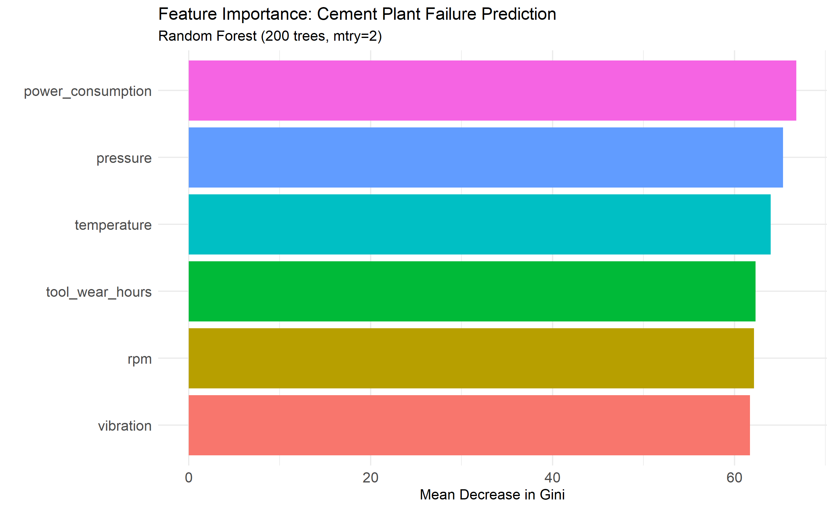
importance_df <- data.frame(
  Feature = rownames(importance(rf_model)),
  Importance = importance(rf_model)[, "MeanDecreaseGini"]
) |>
  arrange(desc(Importance)) |>
  mutate(Feature = fct_reorder(Feature, Importance))

cat("\nFeature Importance (Gini-based):\n")
#> 
#> Feature Importance (Gini-based):
print(importance_df)
#>                             Feature Importance
#> power_consumption power_consumption   66.80715
#> pressure                   pressure   65.33287
#> temperature             temperature   63.99488
#> tool_wear_hours     tool_wear_hours   62.32980
#> rpm                             rpm   62.15375
#> vibration                 vibration   61.69630

# Plot
ggplot(importance_df, aes(x = Importance, y = Feature, fill = Feature)) +
  geom_col(show.legend = FALSE) +
  labs(title = "Feature Importance: Cement Plant Failure Prediction",
       subtitle = "Random Forest (200 trees, mtry=2)",
       x = "Mean Decrease in Gini", y = "") +
  theme_minimal() +
  theme(axis.text = element_text(size = 11))

Python

import numpy as np
import pandas as pd
import matplotlib.pyplot as plt
from sklearn.ensemble import RandomForestClassifier
from sklearn.model_selection import train_test_split

# Synthetic cement plant dataset
np.random.seed(2026)

n_sensors = 2000

cement_data = pd.DataFrame({
    'temperature': np.random.normal(150, 20, n_sensors),
    'vibration': np.random.gamma(2, 5, n_sensors),
    'power_consumption': np.random.normal(2500, 300, n_sensors),
    'rpm': np.random.normal(1200, 100, n_sensors),
    'pressure': np.random.normal(100, 15, n_sensors),
    'tool_wear_hours': np.random.randint(0, 8001, n_sensors),
    'failure_7d': np.random.choice([0, 1], n_sensors, p=[0.88, 0.12])
})

X = cement_data.drop('failure_7d', axis=1)
y = cement_data['failure_7d']

print("Cement plant predictive maintenance dataset")
#> Cement plant predictive maintenance dataset
print(f"Shape: {X.shape}")
#> Shape: (2000, 6)
print(f"Failure rate: {y.mean():.4f}\n")
#> Failure rate: 0.1190

# Train Random Forest
rf_model = RandomForestClassifier(
    n_estimators=200,
    max_features=2,
    max_depth=20,
    min_samples_split=5,
    oob_score=True,
    random_state=2026
)

rf_model.fit(X, y)
#> RandomForestClassifier(max_depth=20, max_features=2, min_samples_split=5,
#>                        n_estimators=200, oob_score=True, random_state=2026)

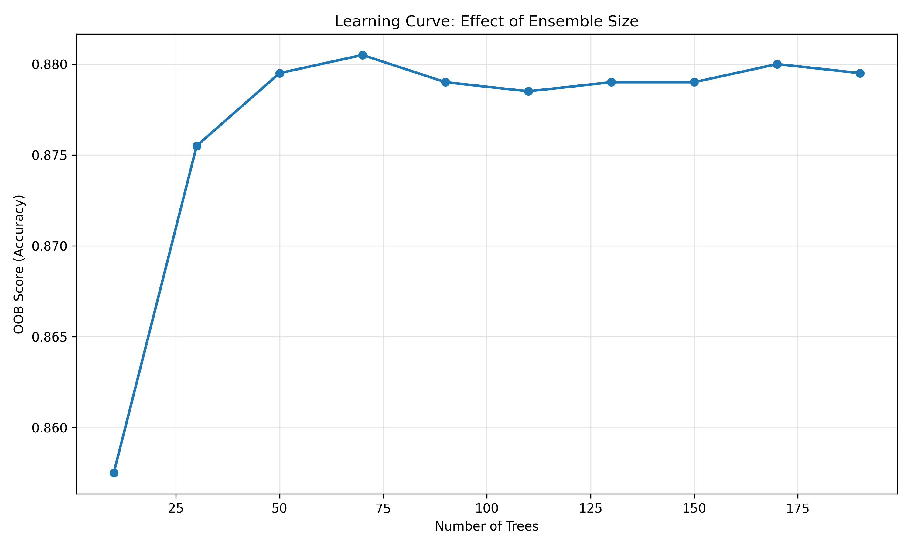
print(f"OOB Score: {rf_model.oob_score_:.4f}")
#> OOB Score: 0.8795
print(f"OOB Error: {1 - rf_model.oob_score_:.4f}\n")
#> OOB Error: 0.1205

# Feature importance
feature_imp = pd.DataFrame({
    'Feature': X.columns,
    'Importance': rf_model.feature_importances_
}).sort_values('Importance', ascending=False)

print("Feature Importance (Gini-based):")
#> Feature Importance (Gini-based):
print(feature_imp)
#>              Feature  Importance
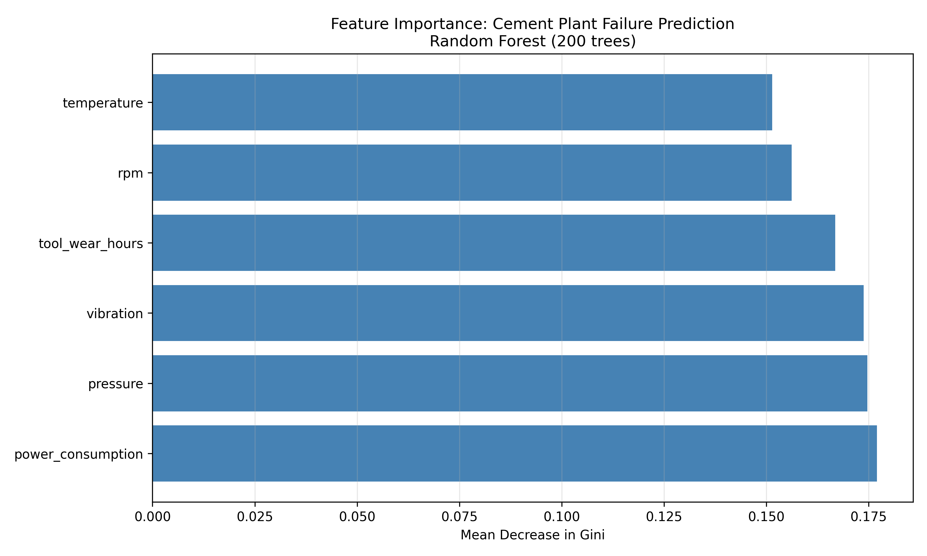
#> 2  power_consumption    0.177020
#> 4           pressure    0.174721
#> 1          vibration    0.173787
#> 5    tool_wear_hours    0.166824
#> 3                rpm    0.156206
#> 0        temperature    0.151441

# Plot
fig, ax = plt.subplots(figsize=(10, 6))
ax.barh(feature_imp['Feature'], feature_imp['Importance'], color='steelblue')
#> <BarContainer object of 6 artists>
ax.set_xlabel('Mean Decrease in Gini')
#> Text(0.5, 0, 'Mean Decrease in Gini')
ax.set_title('Feature Importance: Cement Plant Failure Prediction\nRandom Forest (200 trees)')
#> Text(0.5, 1.0, 'Feature Importance: Cement Plant Failure Prediction\nRandom Forest (200 trees)')
ax.grid(axis='x', alpha=0.3)
plt.tight_layout()
plt.savefig('rf_importance.png', dpi=100, bbox_inches='tight')
plt.show()

# Learning curve: effect of number of trees
from sklearn.metrics import roc_auc_score

n_trees_range = range(10, 210, 20)
oob_scores = []

for n_trees in n_trees_range:
    rf = RandomForestClassifier(n_estimators=n_trees, max_features=2,
                                oob_score=True, random_state=2026)
    rf.fit(X, y)
    oob_scores.append(rf.oob_score_)
#> RandomForestClassifier(max_features=2, n_estimators=10, oob_score=True,
#>                        random_state=2026)
#> RandomForestClassifier(max_features=2, n_estimators=30, oob_score=True,
#>                        random_state=2026)
#> RandomForestClassifier(max_features=2, n_estimators=50, oob_score=True,
#>                        random_state=2026)
#> RandomForestClassifier(max_features=2, n_estimators=70, oob_score=True,
#>                        random_state=2026)
#> RandomForestClassifier(max_features=2, n_estimators=90, oob_score=True,
#>                        random_state=2026)
#> RandomForestClassifier(max_features=2, n_estimators=110, oob_score=True,
#>                        random_state=2026)
#> RandomForestClassifier(max_features=2, n_estimators=130, oob_score=True,
#>                        random_state=2026)
#> RandomForestClassifier(max_features=2, n_estimators=150, oob_score=True,
#>                        random_state=2026)
#> RandomForestClassifier(max_features=2, n_estimators=170, oob_score=True,
#>                        random_state=2026)
#> RandomForestClassifier(max_features=2, n_estimators=190, oob_score=True,
#>                        random_state=2026)

fig, ax = plt.subplots(figsize=(10, 6))
ax.plot(n_trees_range, oob_scores, marker='o', linewidth=2, markersize=6)
#> [<matplotlib.lines.Line2D object at 0x00000206CEB09A90>]
ax.set_xlabel('Number of Trees')
#> Text(0.5, 0, 'Number of Trees')
ax.set_ylabel('OOB Score (Accuracy)')
#> Text(0, 0.5, 'OOB Score (Accuracy)')
ax.set_title('Learning Curve: Effect of Ensemble Size')
#> Text(0.5, 1.0, 'Learning Curve: Effect of Ensemble Size')
ax.grid(alpha=0.3)
plt.tight_layout()
plt.savefig('learning_curve_trees.png', dpi=100, bbox_inches='tight')
plt.show()

Caution📝 Section 15.3 Review Questions

1. Why is feature subsampling in Random Forests important for reducing variance?
2. What is the relationship between max_features and tree correlation?
3. Compare impurity-based vs. permutation importance. When is each more appropriate?
4. How does OOB error scale with the number of trees B?
5. In the cement plant example, which feature is most predictive of failure?

20.4 Gradient Boosting: Sequential Ensemble Learning

While bagging and Random Forests build trees in parallel (each independently), boosting builds trees sequentially, each correcting the residuals of the previous one.

Note📘 Theory: Gradient Boosting

Gradient boosting algorithm:

f_0(x) ← mean of y (initialization)

for m = 1 to M:
    r_i ← y_i - f_{m-1}(x_i)  (compute residuals)
    tree_m ← fit regression tree to (X, r_i)
    f_m(x) ← f_{m-1}(x) + η * tree_m(x)  (add scaled tree to ensemble)
            (η is the learning rate, typically 0.01 to 0.3)

final_prediction(x) ← f_M(x)

Intuition: 1. Start with a simple prediction (mean). 2. Fit a tree to the residuals (differences between actual and predicted). 3. Add this tree’s predictions to the ensemble, scaled by learning rate η. 4. Repeat: each new tree fixes mistakes of the ensemble so far.

Why it works: - Boosting reduces bias (not just variance) by explicitly targeting hard-to-fit samples. - The learning rate η prevents overfitting by taking smaller steps. - Shallow trees (usually depth 3–8) are preferred to avoid overfitting.

Key hyperparameters: - n_estimators (M): Number of boosting rounds. Larger = more complex model, more risk of overfitting. - learning_rate (η): Step size. Lower η (0.01–0.05) requires more trees but often generalizes better. - max_depth: Tree depth, typically 3–8. Shallow trees reduce variance. - subsample: Fraction of samples used to fit each tree (stochastic boosting). - colsample_bytree: Fraction of features used per tree.

Regularisation in boosting: To prevent overfitting: - Reduce η (require more iterations but smaller steps). - Limit tree depth (max_depth). - Use subsampling (subsample, colsample_bytree). - Early stopping: monitor validation error and stop when it plateaus.

Tip🔑 Key Formula: Gradient Boosting Update

\[f_m(x) = f_{m-1}(x) + \eta \cdot tree_m(x)\]

where \(tree_m(x)\) predicts the residuals \(r_i = y_i - f_{m-1}(x_i)\) and \(\eta \in (0, 1]\) is the learning rate.

20.4.1 XGBoost on Cement Plant Data

R

library(xgboost)
library(tidyverse)

# Prepare data for XGBoost
X_matrix <- as.matrix(cement_data[, c("temperature", "vibration",
                                       "power_consumption", "rpm",
                                       "pressure", "tool_wear_hours")])
y_vector <- as.numeric(cement_data$failure_7d) - 1  # Convert to 0/1

# Create xgb.DMatrix
dtrain <- xgb.DMatrix(data = X_matrix, label = y_vector)

# Train XGBoost
xgb_model <- xgb.train(
  params = list(
    objective = "binary:logistic",
    eval_metric = "logloss",
    eta = 0.1,                  # learning rate
    max_depth = 5,
    subsample = 0.8,
    colsample_bytree = 0.8,
    lambda = 1,                 # L2 regularisation
    alpha = 0                   # L1 regularisation
  ),
  data = dtrain,
  nrounds = 100,
  verbose = 0
)

cat("XGBoost model trained (100 rounds)\n\n")
#> XGBoost model trained (100 rounds)

# Feature importance
importance_xgb <- xgb.importance(
  feature_names = colnames(X_matrix),
  model = xgb_model
)

cat("Feature Importance (Gain):\n")
#> Feature Importance (Gain):
print(importance_xgb)
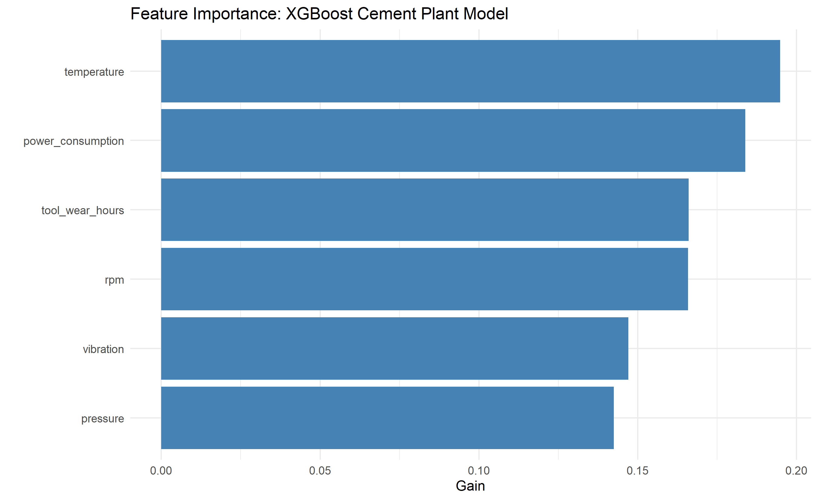
#>              Feature      Gain     Cover Frequency
#>               <char>     <num>     <num>     <num>
#> 1:       temperature 0.1947935 0.1881792 0.1890173
#> 2: power_consumption 0.1838949 0.1683614 0.1757225
#> 3:   tool_wear_hours 0.1660210 0.1749699 0.1635838
#> 4:               rpm 0.1658069 0.1532540 0.1624277
#> 5:         vibration 0.1470136 0.1573593 0.1612717
#> 6:          pressure 0.1424700 0.1578761 0.1479769

# Plot
ggplot(as.data.frame(importance_xgb), aes(x = reorder(Feature, Gain), y = Gain)) +
  geom_col(fill = "steelblue") +
  coord_flip() +
  labs(title = "Feature Importance: XGBoost Cement Plant Model",
       x = "", y = "Gain") +
  theme_minimal()

Python

import xgboost as xgb

# Prepare data
X_matrix = X.values
y_vector = y.values

# Create DMatrix
dtrain = xgb.DMatrix(X_matrix, label=y_vector)

# Train XGBoost
xgb_params = {
    'objective': 'binary:logistic',
    'eval_metric': 'logloss',
    'eta': 0.1,
    'max_depth': 5,
    'subsample': 0.8,
    'colsample_bytree': 0.8,
    'lambda': 1,
    'alpha': 0
}

xgb_model = xgb.train(
    xgb_params,
    dtrain,
    num_boost_round=100,
    verbose_eval=False
)

print("XGBoost model trained (100 rounds)\n")
#> XGBoost model trained (100 rounds)

# Feature importance
importance_xgb = xgb_model.get_score(importance_type='gain')
importance_df_xgb = pd.DataFrame(
    list(importance_xgb.items()),
    columns=['Feature', 'Importance']
).sort_values('Importance', ascending=False)

print("Feature Importance (Gain):")
#> Feature Importance (Gain):
print(importance_df_xgb)
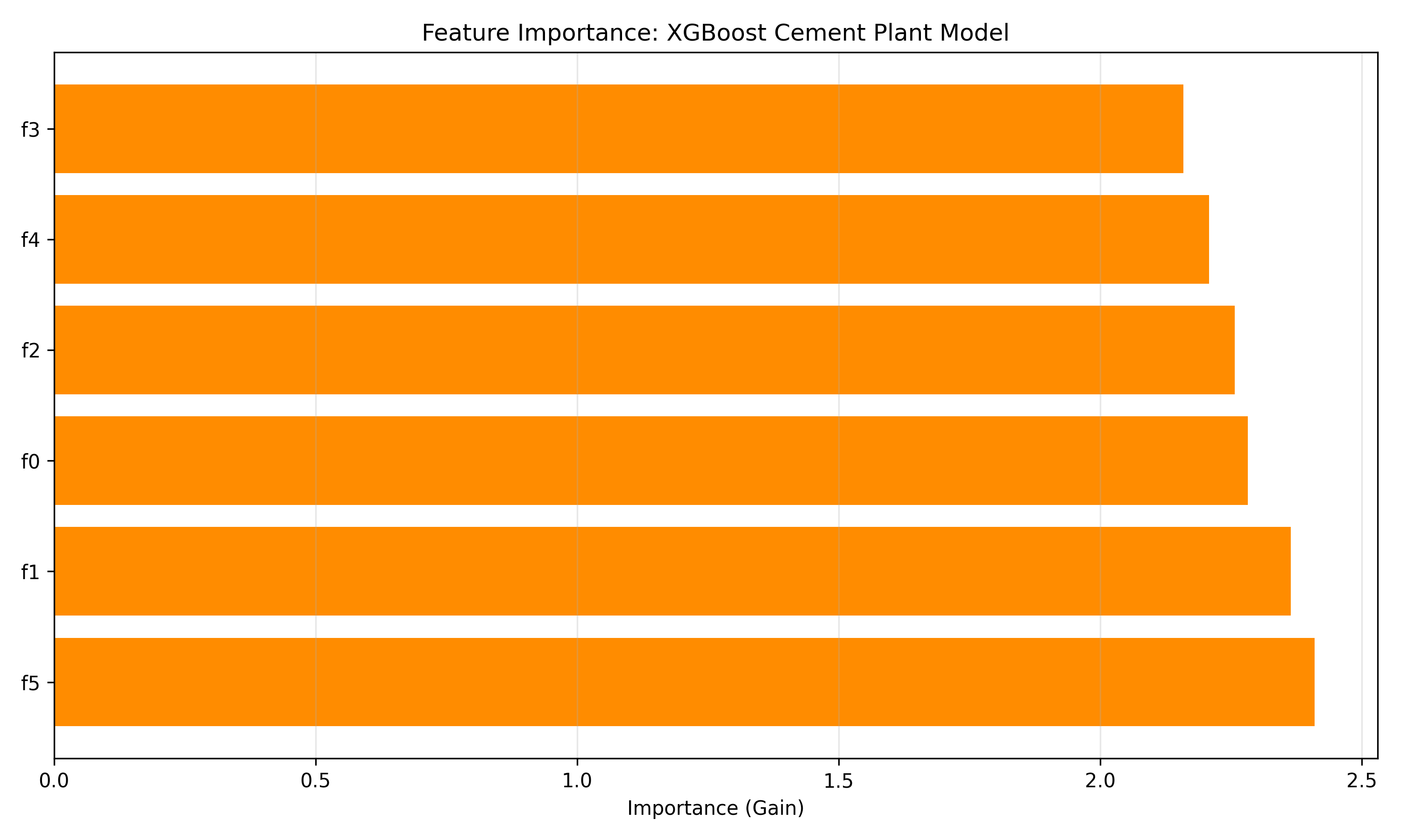
#>   Feature  Importance
#> 5      f5    2.410021
#> 1      f1    2.364471
#> 0      f0    2.282440
#> 2      f2    2.256969
#> 4      f4    2.208287
#> 3      f3    2.159261

# Plot
fig, ax = plt.subplots(figsize=(10, 6))
ax.barh(importance_df_xgb['Feature'], importance_df_xgb['Importance'], color='darkorange')
#> <BarContainer object of 6 artists>
ax.set_xlabel('Importance (Gain)')
#> Text(0.5, 0, 'Importance (Gain)')
ax.set_title('Feature Importance: XGBoost Cement Plant Model')
#> Text(0.5, 1.0, 'Feature Importance: XGBoost Cement Plant Model')
ax.grid(axis='x', alpha=0.3)
plt.tight_layout()
plt.savefig('xgb_importance.png', dpi=100, bbox_inches='tight')
plt.show()

Caution📝 Section 15.4 Review Questions

1. Why does boosting address bias while bagging addresses variance?
2. Explain the effect of learning rate η. What happens if η is too small? Too large?
3. In gradient boosting, why do we fit trees to residuals rather than the original y?
4. How does tree depth in boosting differ from Random Forests?

20.5 XGBoost and LightGBM: Modern Implementations

Modern gradient boosting libraries add regularisation, GPU acceleration, and histogram-based splits for efficiency.

Note📘 Theory: Advances in Gradient Boosting

XGBoost (eXtreme Gradient Boosting): - Regularised objective: \[L = \sum_{i=1}^{n} l(y_i, \hat{y}_i) + \sum_{t=1}^{T} \Omega(f_t)\] where Ω(f) = γT + λ||w||² is a regulariser on tree structure and weights. - Second-order derivatives: Newton boosting uses both gradient and Hessian for more stable updates. - Column subsampling: Reduces overfitting. - Weighted quantile sketch: For efficient split finding.

LightGBM (Light Gradient Boosting Machine): - Histogram-based splits: Bins features into ~256 bins, speeds up split finding 10×. - Leaf-wise growth: Grows trees by maximizing loss reduction (different from level-wise growth), often achieving better fit with fewer trees. - GPU support: Native CUDA support for large datasets. - Categorical feature support: Handles categorical variables natively without one-hot encoding.

Comparison:

Aspect	Random Forest	XGBoost	LightGBM
Speed	Fast	Medium	Very fast (histogram + GPU)
Memory	Moderate	High	Low
Default depth	Unlimited	6	31
Regularisation	None (implicit OOB)	L1/L2 + tree structure	L1/L2 + tree structure
Interpretability	High	Medium	Medium

20.5.1 Hyperparameter Grid Search with CV

R

library(xgboost)
library(tidyverse)

# Set up train/test split
set.seed(2026)
train_idx <- sample(1:nrow(cement_data), 0.7 * nrow(cement_data))

X_train <- as.matrix(cement_data[train_idx, c("temperature", "vibration",
                                               "power_consumption", "rpm",
                                               "pressure", "tool_wear_hours")])
X_test <- as.matrix(cement_data[-train_idx, c("temperature", "vibration",
                                               "power_consumption", "rpm",
                                               "pressure", "tool_wear_hours")])

y_train <- as.numeric(cement_data$failure_7d[train_idx]) - 1
y_test <- as.numeric(cement_data$failure_7d[-train_idx]) - 1

dtrain <- xgb.DMatrix(X_train, label = y_train)
dtest <- xgb.DMatrix(X_test, label = y_test)

# Hyperparameter grid
param_grid <- expand.grid(
  eta = c(0.01, 0.05, 0.1),
  max_depth = c(3, 5, 7),
  subsample = c(0.7, 0.8, 0.9)
)

cat("Grid search: ", nrow(param_grid), "parameter combinations\n\n")
#> Grid search:  27 parameter combinations

results <- list()

for (i in 1:nrow(param_grid)) {
  params <- list(
    objective = "binary:logistic",
    eval_metric = "auc",
    eta = param_grid$eta[i],
    max_depth = param_grid$max_depth[i],
    subsample = param_grid$subsample[i],
    lambda = 1,
    alpha = 0
  )

  # Train model (fixed nrounds — avoids evaluation_log version fragility)
  model <- xgb.train(
    params = params,
    data   = dtrain,
    nrounds = 100,
    verbose = 0
  )

  # Compute AUC directly from predictions — works on every xgboost version
  pred_tmp   <- predict(model, dtest)
  best_score <- as.numeric(pROC::auc(pROC::roc(y_test, pred_tmp, quiet = TRUE)))
  results[[i]] <- data.frame(
    eta       = param_grid$eta[i],
    max_depth = param_grid$max_depth[i],
    subsample = param_grid$subsample[i],
    best_auc  = best_score,
    best_round = 100L
  )
}

results_df <- bind_rows(results) |>
  arrange(desc(best_auc))

cat("Top 5 parameter combinations:\n")
#> Top 5 parameter combinations:
print(head(results_df, 5))
#>    eta max_depth subsample  best_auc best_round
#> 1 0.05         5       0.7 0.5440071        100
#> 2 0.10         5       0.9 0.5301858        100
#> 3 0.10         5       0.8 0.5235792        100
#> 4 0.01         3       0.9 0.5222800        100
#> 5 0.10         7       0.9 0.5217824        100

# Retrain best model
best_params <- results_df[1, ]
best_model <- xgb.train(
  params = list(
    objective = "binary:logistic",
    eval_metric = "auc",
    eta = best_params$eta,
    max_depth = best_params$max_depth,
    subsample = best_params$subsample,
    lambda = 1
  ),
  data = dtrain,
  nrounds = best_params$best_round,
  verbose = 0
)

# Test predictions
test_pred <- predict(best_model, dtest)
test_auc <- pROC::auc(y_test, test_pred)

cat("\nBest model test AUC:", round(test_auc, 4), "\n")
#> 
#> Best model test AUC: 0.5138

Python

from sklearn.model_selection import GridSearchCV
from sklearn.metrics import roc_auc_score, roc_curve
from xgboost import XGBClassifier
import itertools

# Train-test split
X_train, X_test, y_train, y_test = train_test_split(
    X, y, test_size=0.3, random_state=2026
)

# Parameter grid
param_grid = {
    'eta': [0.01, 0.05, 0.1],
    'max_depth': [3, 5, 7],
    'subsample': [0.7, 0.8, 0.9]
}

print(f"Grid search: {np.prod([len(v) for v in param_grid.values()])} combinations\n")
#> Grid search: 27 combinations

# Manual grid search with early stopping
results = []

for eta in param_grid['eta']:
    for max_depth in param_grid['max_depth']:
        for subsample in param_grid['subsample']:
            xgb = XGBClassifier(
                n_estimators=200,
                eta=eta,
                max_depth=max_depth,
                subsample=subsample,
                lambda_=1,
                alpha=0,
                early_stopping_rounds=10,
                eval_metric='logloss',
                random_state=2026
            )

            xgb.fit(X_train, y_train, eval_set=[(X_test, y_test)], verbose=False)

            y_pred_train = xgb.predict_proba(X_train)[:, 1]
            y_pred_test = xgb.predict_proba(X_test)[:, 1]

            auc_train = roc_auc_score(y_train, y_pred_train)
            auc_test = roc_auc_score(y_test, y_pred_test)

            results.append({
                'eta': eta,
                'max_depth': max_depth,
                'subsample': subsample,
                'auc_train': auc_train,
                'auc_test': auc_test,
                'n_rounds': xgb.best_ntree_limit if hasattr(xgb, 'best_ntree_limit') else xgb.n_estimators
            })
#> XGBClassifier(alpha=0, base_score=None, booster=None, callbacks=None,
#>               colsample_bylevel=None, colsample_bynode=None,
#>               colsample_bytree=None, device=None, early_stopping_rounds=10,
#>               enable_categorical=False, eta=0.01, eval_metric='logloss',
#>               feature_types=None, feature_weights=None, gamma=None,
#>               grow_policy=None, importance_type=None,
#>               interaction_constraints=None, lambda_=1, learning_rate=None,
#>               max_bin=None, max_cat_threshold=None, max_cat_to_onehot=None,
#>               max_delta_step=None, max_depth=3, max_leaves=None,
#>               min_child_weight=None, missing=nan, monotone_constraints=None,
#>               multi_strategy=None, ...)
#> XGBClassifier(alpha=0, base_score=None, booster=None, callbacks=None,
#>               colsample_bylevel=None, colsample_bynode=None,
#>               colsample_bytree=None, device=None, early_stopping_rounds=10,
#>               enable_categorical=False, eta=0.01, eval_metric='logloss',
#>               feature_types=None, feature_weights=None, gamma=None,
#>               grow_policy=None, importance_type=None,
#>               interaction_constraints=None, lambda_=1, learning_rate=None,
#>               max_bin=None, max_cat_threshold=None, max_cat_to_onehot=None,
#>               max_delta_step=None, max_depth=3, max_leaves=None,
#>               min_child_weight=None, missing=nan, monotone_constraints=None,
#>               multi_strategy=None, ...)
#> XGBClassifier(alpha=0, base_score=None, booster=None, callbacks=None,
#>               colsample_bylevel=None, colsample_bynode=None,
#>               colsample_bytree=None, device=None, early_stopping_rounds=10,
#>               enable_categorical=False, eta=0.01, eval_metric='logloss',
#>               feature_types=None, feature_weights=None, gamma=None,
#>               grow_policy=None, importance_type=None,
#>               interaction_constraints=None, lambda_=1, learning_rate=None,
#>               max_bin=None, max_cat_threshold=None, max_cat_to_onehot=None,
#>               max_delta_step=None, max_depth=3, max_leaves=None,
#>               min_child_weight=None, missing=nan, monotone_constraints=None,
#>               multi_strategy=None, ...)
#> XGBClassifier(alpha=0, base_score=None, booster=None, callbacks=None,
#>               colsample_bylevel=None, colsample_bynode=None,
#>               colsample_bytree=None, device=None, early_stopping_rounds=10,
#>               enable_categorical=False, eta=0.01, eval_metric='logloss',
#>               feature_types=None, feature_weights=None, gamma=None,
#>               grow_policy=None, importance_type=None,
#>               interaction_constraints=None, lambda_=1, learning_rate=None,
#>               max_bin=None, max_cat_threshold=None, max_cat_to_onehot=None,
#>               max_delta_step=None, max_depth=5, max_leaves=None,
#>               min_child_weight=None, missing=nan, monotone_constraints=None,
#>               multi_strategy=None, ...)
#> XGBClassifier(alpha=0, base_score=None, booster=None, callbacks=None,
#>               colsample_bylevel=None, colsample_bynode=None,
#>               colsample_bytree=None, device=None, early_stopping_rounds=10,
#>               enable_categorical=False, eta=0.01, eval_metric='logloss',
#>               feature_types=None, feature_weights=None, gamma=None,
#>               grow_policy=None, importance_type=None,
#>               interaction_constraints=None, lambda_=1, learning_rate=None,
#>               max_bin=None, max_cat_threshold=None, max_cat_to_onehot=None,
#>               max_delta_step=None, max_depth=5, max_leaves=None,
#>               min_child_weight=None, missing=nan, monotone_constraints=None,
#>               multi_strategy=None, ...)
#> XGBClassifier(alpha=0, base_score=None, booster=None, callbacks=None,
#>               colsample_bylevel=None, colsample_bynode=None,
#>               colsample_bytree=None, device=None, early_stopping_rounds=10,
#>               enable_categorical=False, eta=0.01, eval_metric='logloss',
#>               feature_types=None, feature_weights=None, gamma=None,
#>               grow_policy=None, importance_type=None,
#>               interaction_constraints=None, lambda_=1, learning_rate=None,
#>               max_bin=None, max_cat_threshold=None, max_cat_to_onehot=None,
#>               max_delta_step=None, max_depth=5, max_leaves=None,
#>               min_child_weight=None, missing=nan, monotone_constraints=None,
#>               multi_strategy=None, ...)
#> XGBClassifier(alpha=0, base_score=None, booster=None, callbacks=None,
#>               colsample_bylevel=None, colsample_bynode=None,
#>               colsample_bytree=None, device=None, early_stopping_rounds=10,
#>               enable_categorical=False, eta=0.01, eval_metric='logloss',
#>               feature_types=None, feature_weights=None, gamma=None,
#>               grow_policy=None, importance_type=None,
#>               interaction_constraints=None, lambda_=1, learning_rate=None,
#>               max_bin=None, max_cat_threshold=None, max_cat_to_onehot=None,
#>               max_delta_step=None, max_depth=7, max_leaves=None,
#>               min_child_weight=None, missing=nan, monotone_constraints=None,
#>               multi_strategy=None, ...)
#> XGBClassifier(alpha=0, base_score=None, booster=None, callbacks=None,
#>               colsample_bylevel=None, colsample_bynode=None,
#>               colsample_bytree=None, device=None, early_stopping_rounds=10,
#>               enable_categorical=False, eta=0.01, eval_metric='logloss',
#>               feature_types=None, feature_weights=None, gamma=None,
#>               grow_policy=None, importance_type=None,
#>               interaction_constraints=None, lambda_=1, learning_rate=None,
#>               max_bin=None, max_cat_threshold=None, max_cat_to_onehot=None,
#>               max_delta_step=None, max_depth=7, max_leaves=None,
#>               min_child_weight=None, missing=nan, monotone_constraints=None,
#>               multi_strategy=None, ...)
#> XGBClassifier(alpha=0, base_score=None, booster=None, callbacks=None,
#>               colsample_bylevel=None, colsample_bynode=None,
#>               colsample_bytree=None, device=None, early_stopping_rounds=10,
#>               enable_categorical=False, eta=0.01, eval_metric='logloss',
#>               feature_types=None, feature_weights=None, gamma=None,
#>               grow_policy=None, importance_type=None,
#>               interaction_constraints=None, lambda_=1, learning_rate=None,
#>               max_bin=None, max_cat_threshold=None, max_cat_to_onehot=None,
#>               max_delta_step=None, max_depth=7, max_leaves=None,
#>               min_child_weight=None, missing=nan, monotone_constraints=None,
#>               multi_strategy=None, ...)
#> XGBClassifier(alpha=0, base_score=None, booster=None, callbacks=None,
#>               colsample_bylevel=None, colsample_bynode=None,
#>               colsample_bytree=None, device=None, early_stopping_rounds=10,
#>               enable_categorical=False, eta=0.05, eval_metric='logloss',
#>               feature_types=None, feature_weights=None, gamma=None,
#>               grow_policy=None, importance_type=None,
#>               interaction_constraints=None, lambda_=1, learning_rate=None,
#>               max_bin=None, max_cat_threshold=None, max_cat_to_onehot=None,
#>               max_delta_step=None, max_depth=3, max_leaves=None,
#>               min_child_weight=None, missing=nan, monotone_constraints=None,
#>               multi_strategy=None, ...)
#> XGBClassifier(alpha=0, base_score=None, booster=None, callbacks=None,
#>               colsample_bylevel=None, colsample_bynode=None,
#>               colsample_bytree=None, device=None, early_stopping_rounds=10,
#>               enable_categorical=False, eta=0.05, eval_metric='logloss',
#>               feature_types=None, feature_weights=None, gamma=None,
#>               grow_policy=None, importance_type=None,
#>               interaction_constraints=None, lambda_=1, learning_rate=None,
#>               max_bin=None, max_cat_threshold=None, max_cat_to_onehot=None,
#>               max_delta_step=None, max_depth=3, max_leaves=None,
#>               min_child_weight=None, missing=nan, monotone_constraints=None,
#>               multi_strategy=None, ...)
#> XGBClassifier(alpha=0, base_score=None, booster=None, callbacks=None,
#>               colsample_bylevel=None, colsample_bynode=None,
#>               colsample_bytree=None, device=None, early_stopping_rounds=10,
#>               enable_categorical=False, eta=0.05, eval_metric='logloss',
#>               feature_types=None, feature_weights=None, gamma=None,
#>               grow_policy=None, importance_type=None,
#>               interaction_constraints=None, lambda_=1, learning_rate=None,
#>               max_bin=None, max_cat_threshold=None, max_cat_to_onehot=None,
#>               max_delta_step=None, max_depth=3, max_leaves=None,
#>               min_child_weight=None, missing=nan, monotone_constraints=None,
#>               multi_strategy=None, ...)
#> XGBClassifier(alpha=0, base_score=None, booster=None, callbacks=None,
#>               colsample_bylevel=None, colsample_bynode=None,
#>               colsample_bytree=None, device=None, early_stopping_rounds=10,
#>               enable_categorical=False, eta=0.05, eval_metric='logloss',
#>               feature_types=None, feature_weights=None, gamma=None,
#>               grow_policy=None, importance_type=None,
#>               interaction_constraints=None, lambda_=1, learning_rate=None,
#>               max_bin=None, max_cat_threshold=None, max_cat_to_onehot=None,
#>               max_delta_step=None, max_depth=5, max_leaves=None,
#>               min_child_weight=None, missing=nan, monotone_constraints=None,
#>               multi_strategy=None, ...)
#> XGBClassifier(alpha=0, base_score=None, booster=None, callbacks=None,
#>               colsample_bylevel=None, colsample_bynode=None,
#>               colsample_bytree=None, device=None, early_stopping_rounds=10,
#>               enable_categorical=False, eta=0.05, eval_metric='logloss',
#>               feature_types=None, feature_weights=None, gamma=None,
#>               grow_policy=None, importance_type=None,
#>               interaction_constraints=None, lambda_=1, learning_rate=None,
#>               max_bin=None, max_cat_threshold=None, max_cat_to_onehot=None,
#>               max_delta_step=None, max_depth=5, max_leaves=None,
#>               min_child_weight=None, missing=nan, monotone_constraints=None,
#>               multi_strategy=None, ...)
#> XGBClassifier(alpha=0, base_score=None, booster=None, callbacks=None,
#>               colsample_bylevel=None, colsample_bynode=None,
#>               colsample_bytree=None, device=None, early_stopping_rounds=10,
#>               enable_categorical=False, eta=0.05, eval_metric='logloss',
#>               feature_types=None, feature_weights=None, gamma=None,
#>               grow_policy=None, importance_type=None,
#>               interaction_constraints=None, lambda_=1, learning_rate=None,
#>               max_bin=None, max_cat_threshold=None, max_cat_to_onehot=None,
#>               max_delta_step=None, max_depth=5, max_leaves=None,
#>               min_child_weight=None, missing=nan, monotone_constraints=None,
#>               multi_strategy=None, ...)
#> XGBClassifier(alpha=0, base_score=None, booster=None, callbacks=None,
#>               colsample_bylevel=None, colsample_bynode=None,
#>               colsample_bytree=None, device=None, early_stopping_rounds=10,
#>               enable_categorical=False, eta=0.05, eval_metric='logloss',
#>               feature_types=None, feature_weights=None, gamma=None,
#>               grow_policy=None, importance_type=None,
#>               interaction_constraints=None, lambda_=1, learning_rate=None,
#>               max_bin=None, max_cat_threshold=None, max_cat_to_onehot=None,
#>               max_delta_step=None, max_depth=7, max_leaves=None,
#>               min_child_weight=None, missing=nan, monotone_constraints=None,
#>               multi_strategy=None, ...)
#> XGBClassifier(alpha=0, base_score=None, booster=None, callbacks=None,
#>               colsample_bylevel=None, colsample_bynode=None,
#>               colsample_bytree=None, device=None, early_stopping_rounds=10,
#>               enable_categorical=False, eta=0.05, eval_metric='logloss',
#>               feature_types=None, feature_weights=None, gamma=None,
#>               grow_policy=None, importance_type=None,
#>               interaction_constraints=None, lambda_=1, learning_rate=None,
#>               max_bin=None, max_cat_threshold=None, max_cat_to_onehot=None,
#>               max_delta_step=None, max_depth=7, max_leaves=None,
#>               min_child_weight=None, missing=nan, monotone_constraints=None,
#>               multi_strategy=None, ...)
#> XGBClassifier(alpha=0, base_score=None, booster=None, callbacks=None,
#>               colsample_bylevel=None, colsample_bynode=None,
#>               colsample_bytree=None, device=None, early_stopping_rounds=10,
#>               enable_categorical=False, eta=0.05, eval_metric='logloss',
#>               feature_types=None, feature_weights=None, gamma=None,
#>               grow_policy=None, importance_type=None,
#>               interaction_constraints=None, lambda_=1, learning_rate=None,
#>               max_bin=None, max_cat_threshold=None, max_cat_to_onehot=None,
#>               max_delta_step=None, max_depth=7, max_leaves=None,
#>               min_child_weight=None, missing=nan, monotone_constraints=None,
#>               multi_strategy=None, ...)
#> XGBClassifier(alpha=0, base_score=None, booster=None, callbacks=None,
#>               colsample_bylevel=None, colsample_bynode=None,
#>               colsample_bytree=None, device=None, early_stopping_rounds=10,
#>               enable_categorical=False, eta=0.1, eval_metric='logloss',
#>               feature_types=None, feature_weights=None, gamma=None,
#>               grow_policy=None, importance_type=None,
#>               interaction_constraints=None, lambda_=1, learning_rate=None,
#>               max_bin=None, max_cat_threshold=None, max_cat_to_onehot=None,
#>               max_delta_step=None, max_depth=3, max_leaves=None,
#>               min_child_weight=None, missing=nan, monotone_constraints=None,
#>               multi_strategy=None, ...)
#> XGBClassifier(alpha=0, base_score=None, booster=None, callbacks=None,
#>               colsample_bylevel=None, colsample_bynode=None,
#>               colsample_bytree=None, device=None, early_stopping_rounds=10,
#>               enable_categorical=False, eta=0.1, eval_metric='logloss',
#>               feature_types=None, feature_weights=None, gamma=None,
#>               grow_policy=None, importance_type=None,
#>               interaction_constraints=None, lambda_=1, learning_rate=None,
#>               max_bin=None, max_cat_threshold=None, max_cat_to_onehot=None,
#>               max_delta_step=None, max_depth=3, max_leaves=None,
#>               min_child_weight=None, missing=nan, monotone_constraints=None,
#>               multi_strategy=None, ...)
#> XGBClassifier(alpha=0, base_score=None, booster=None, callbacks=None,
#>               colsample_bylevel=None, colsample_bynode=None,
#>               colsample_bytree=None, device=None, early_stopping_rounds=10,
#>               enable_categorical=False, eta=0.1, eval_metric='logloss',
#>               feature_types=None, feature_weights=None, gamma=None,
#>               grow_policy=None, importance_type=None,
#>               interaction_constraints=None, lambda_=1, learning_rate=None,
#>               max_bin=None, max_cat_threshold=None, max_cat_to_onehot=None,
#>               max_delta_step=None, max_depth=3, max_leaves=None,
#>               min_child_weight=None, missing=nan, monotone_constraints=None,
#>               multi_strategy=None, ...)
#> XGBClassifier(alpha=0, base_score=None, booster=None, callbacks=None,
#>               colsample_bylevel=None, colsample_bynode=None,
#>               colsample_bytree=None, device=None, early_stopping_rounds=10,
#>               enable_categorical=False, eta=0.1, eval_metric='logloss',
#>               feature_types=None, feature_weights=None, gamma=None,
#>               grow_policy=None, importance_type=None,
#>               interaction_constraints=None, lambda_=1, learning_rate=None,
#>               max_bin=None, max_cat_threshold=None, max_cat_to_onehot=None,
#>               max_delta_step=None, max_depth=5, max_leaves=None,
#>               min_child_weight=None, missing=nan, monotone_constraints=None,
#>               multi_strategy=None, ...)
#> XGBClassifier(alpha=0, base_score=None, booster=None, callbacks=None,
#>               colsample_bylevel=None, colsample_bynode=None,
#>               colsample_bytree=None, device=None, early_stopping_rounds=10,
#>               enable_categorical=False, eta=0.1, eval_metric='logloss',
#>               feature_types=None, feature_weights=None, gamma=None,
#>               grow_policy=None, importance_type=None,
#>               interaction_constraints=None, lambda_=1, learning_rate=None,
#>               max_bin=None, max_cat_threshold=None, max_cat_to_onehot=None,
#>               max_delta_step=None, max_depth=5, max_leaves=None,
#>               min_child_weight=None, missing=nan, monotone_constraints=None,
#>               multi_strategy=None, ...)
#> XGBClassifier(alpha=0, base_score=None, booster=None, callbacks=None,
#>               colsample_bylevel=None, colsample_bynode=None,
#>               colsample_bytree=None, device=None, early_stopping_rounds=10,
#>               enable_categorical=False, eta=0.1, eval_metric='logloss',
#>               feature_types=None, feature_weights=None, gamma=None,
#>               grow_policy=None, importance_type=None,
#>               interaction_constraints=None, lambda_=1, learning_rate=None,
#>               max_bin=None, max_cat_threshold=None, max_cat_to_onehot=None,
#>               max_delta_step=None, max_depth=5, max_leaves=None,
#>               min_child_weight=None, missing=nan, monotone_constraints=None,
#>               multi_strategy=None, ...)
#> XGBClassifier(alpha=0, base_score=None, booster=None, callbacks=None,
#>               colsample_bylevel=None, colsample_bynode=None,
#>               colsample_bytree=None, device=None, early_stopping_rounds=10,
#>               enable_categorical=False, eta=0.1, eval_metric='logloss',
#>               feature_types=None, feature_weights=None, gamma=None,
#>               grow_policy=None, importance_type=None,
#>               interaction_constraints=None, lambda_=1, learning_rate=None,
#>               max_bin=None, max_cat_threshold=None, max_cat_to_onehot=None,
#>               max_delta_step=None, max_depth=7, max_leaves=None,
#>               min_child_weight=None, missing=nan, monotone_constraints=None,
#>               multi_strategy=None, ...)
#> XGBClassifier(alpha=0, base_score=None, booster=None, callbacks=None,
#>               colsample_bylevel=None, colsample_bynode=None,
#>               colsample_bytree=None, device=None, early_stopping_rounds=10,
#>               enable_categorical=False, eta=0.1, eval_metric='logloss',
#>               feature_types=None, feature_weights=None, gamma=None,
#>               grow_policy=None, importance_type=None,
#>               interaction_constraints=None, lambda_=1, learning_rate=None,
#>               max_bin=None, max_cat_threshold=None, max_cat_to_onehot=None,
#>               max_delta_step=None, max_depth=7, max_leaves=None,
#>               min_child_weight=None, missing=nan, monotone_constraints=None,
#>               multi_strategy=None, ...)
#> XGBClassifier(alpha=0, base_score=None, booster=None, callbacks=None,
#>               colsample_bylevel=None, colsample_bynode=None,
#>               colsample_bytree=None, device=None, early_stopping_rounds=10,
#>               enable_categorical=False, eta=0.1, eval_metric='logloss',
#>               feature_types=None, feature_weights=None, gamma=None,
#>               grow_policy=None, importance_type=None,
#>               interaction_constraints=None, lambda_=1, learning_rate=None,
#>               max_bin=None, max_cat_threshold=None, max_cat_to_onehot=None,
#>               max_delta_step=None, max_depth=7, max_leaves=None,
#>               min_child_weight=None, missing=nan, monotone_constraints=None,
#>               multi_strategy=None, ...)

results_df = pd.DataFrame(results).sort_values('auc_test', ascending=False)

print("Top 5 parameter combinations:")
#> Top 5 parameter combinations:
print(results_df.head())
#>      eta  max_depth  subsample  auc_train  auc_test  n_rounds
#> 25  0.10          7        0.8   0.973225  0.607523       200
#> 15  0.05          7        0.7   0.737581  0.585103       200
#> 6   0.01          7        0.7   0.737581  0.585103       200
#> 24  0.10          7        0.7   0.839173  0.577968       200
#> 21  0.10          5        0.7   0.766269  0.560240       200

# Retrain best model
best = results_df.iloc[0]
best_xgb = XGBClassifier(
    n_estimators=int(best['n_rounds']),
    eta=best['eta'],
    max_depth=int(best['max_depth']),
    subsample=best['subsample'],
    lambda_=1,
    random_state=2026
)
best_xgb.fit(X_train, y_train)
#> XGBClassifier(base_score=None, booster=None, callbacks=None,
#>               colsample_bylevel=None, colsample_bynode=None,
#>               colsample_bytree=None, device=None, early_stopping_rounds=None,
#>               enable_categorical=False, eta=np.float64(0.1), eval_metric=None,
#>               feature_types=None, feature_weights=None, gamma=None,
#>               grow_policy=None, importance_type=None,
#>               interaction_constraints=None, lambda_=1, learning_rate=None,
#>               max_bin=None, max_cat_threshold=None, max_cat_to_onehot=None,
#>               max_delta_step=None, max_depth=7, max_leaves=None,
#>               min_child_weight=None, missing=nan, monotone_constraints=None,
#>               multi_strategy=None, n_estimators=200, ...)

y_pred_test = best_xgb.predict_proba(X_test)[:, 1]
test_auc = roc_auc_score(y_test, y_pred_test)

print(f"\nBest model test AUC: {test_auc:.4f}")
#> 
#> Best model test AUC: 0.5869

Caution📝 Section 15.5 Review Questions

1. What regularisation techniques does XGBoost use to prevent overfitting?
2. Why is histogram-based splitting faster than exact split finding?
3. Compare tree growth strategies: level-wise (XGBoost) vs. leaf-wise (LightGBM).
4. When would you choose LightGBM over XGBoost?

20.6 Learning Curves and Hyperparameter Tuning

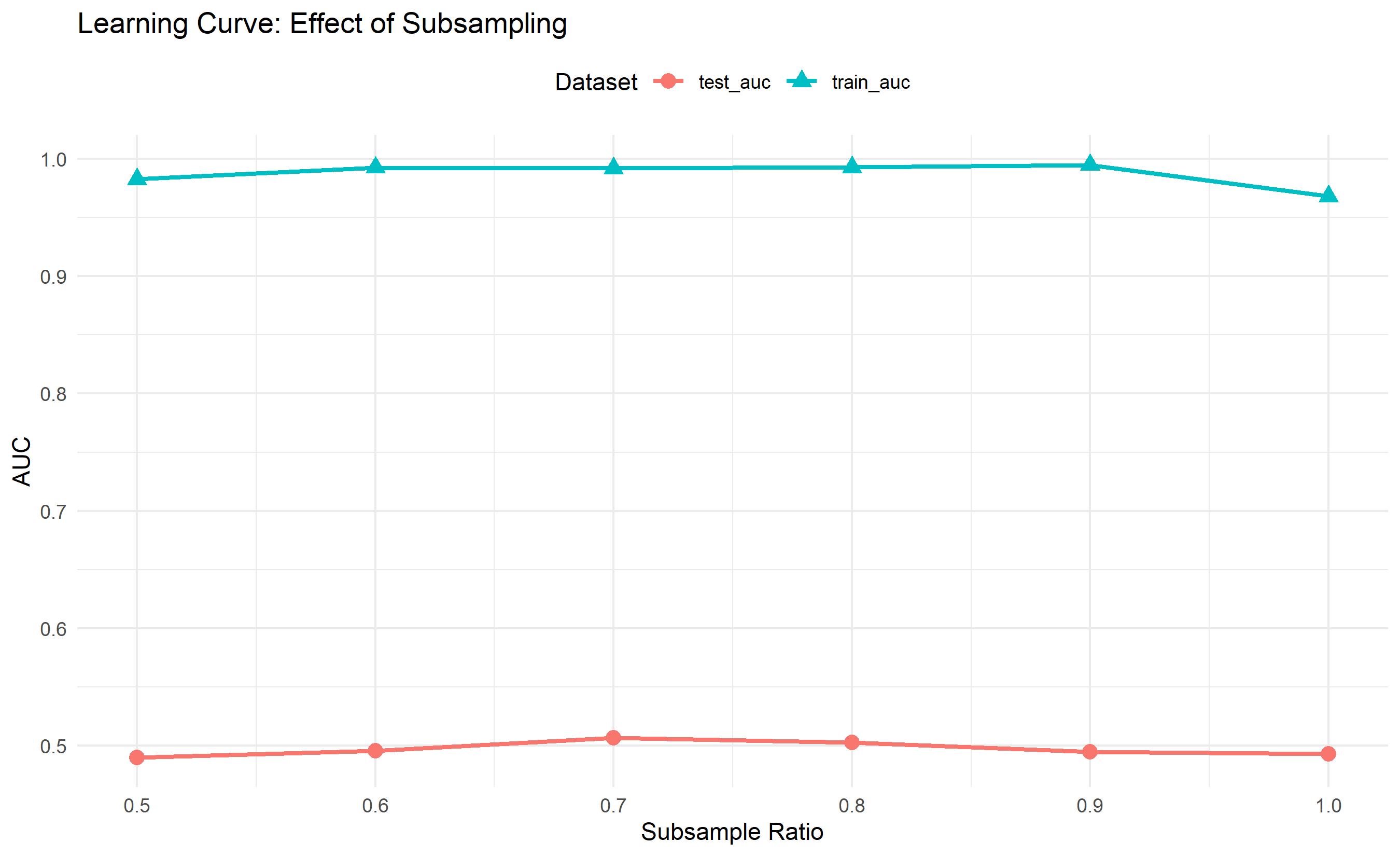
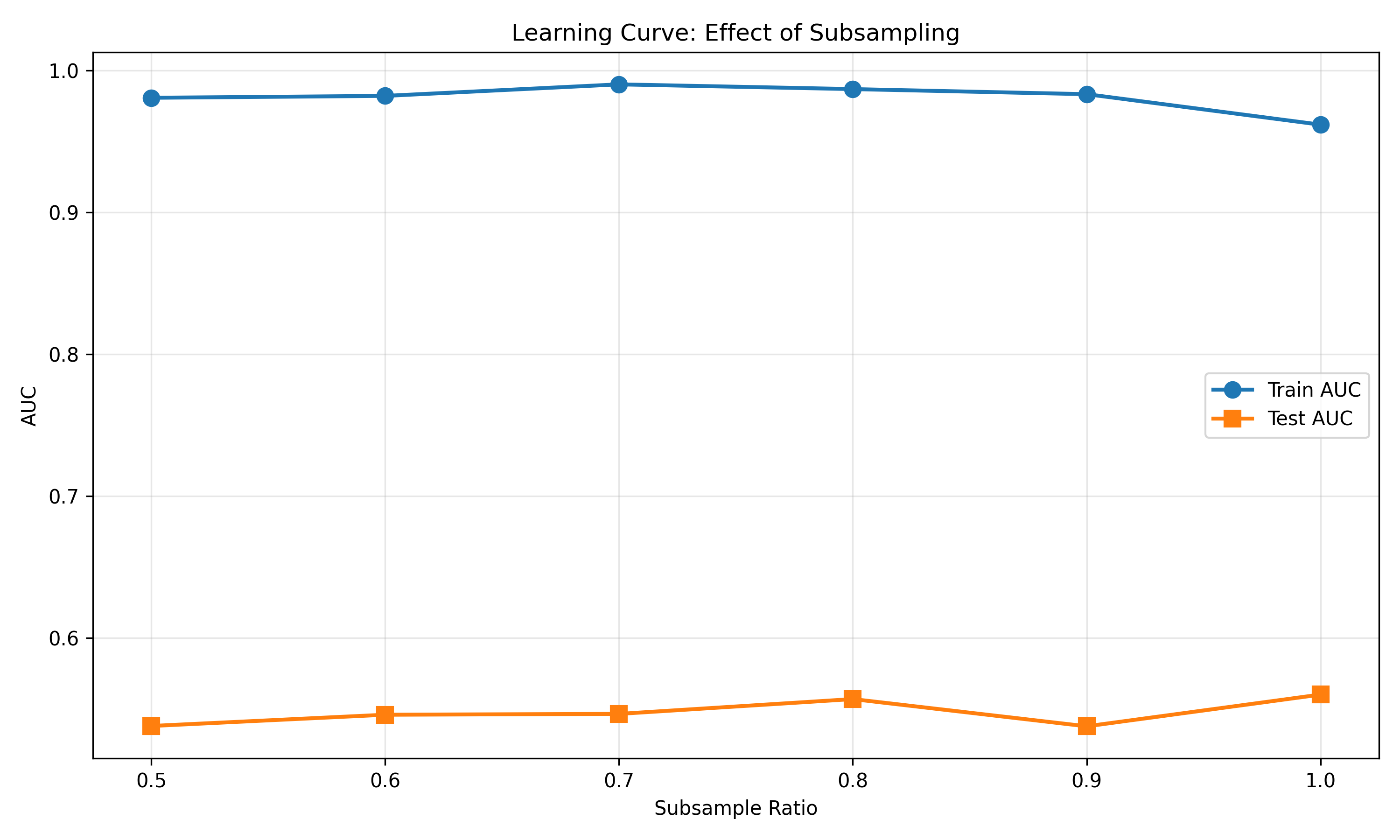
Learning curves help diagnose overfitting and guide hyperparameter selection.

R

# Learning curve: effect of subsample
subsample_values <- seq(0.5, 1.0, by = 0.1)
auc_train <- numeric(length(subsample_values))
auc_test <- numeric(length(subsample_values))

for (i in seq_along(subsample_values)) {
  params <- list(
    objective = "binary:logistic",
    eval_metric = "auc",
    eta = 0.05,
    max_depth = 5,
    subsample = subsample_values[i],
    lambda = 1
  )

  model <- xgb.train(
    params = params,
    data    = dtrain,
    nrounds = 100,
    verbose = 0
  )

  # Compute AUC directly from predictions — avoids evaluation_log version issues
  pred_tr      <- predict(model, dtrain)
  pred_te      <- predict(model, dtest)
  auc_train[i] <- as.numeric(pROC::auc(pROC::roc(y_train, pred_tr, quiet = TRUE)))
  auc_test[i]  <- as.numeric(pROC::auc(pROC::roc(y_test,  pred_te, quiet = TRUE)))
}

learning_curve_df <- data.frame(
  subsample = subsample_values,
  train_auc = auc_train,
  test_auc = auc_test
) |>
  pivot_longer(cols = c(train_auc, test_auc), names_to = "dataset", values_to = "auc")

ggplot(learning_curve_df, aes(x = subsample, y = auc, color = dataset, shape = dataset)) +
  geom_point(size = 3) +
  geom_line(linewidth = 1) +
  labs(title = "Learning Curve: Effect of Subsampling",
       x = "Subsample Ratio", y = "AUC",
       color = "Dataset", shape = "Dataset") +
  theme_minimal() +
  theme(legend.position = "top")

Python

# Learning curve: effect of subsample
from sklearn.metrics import roc_auc_score

subsample_values = np.arange(0.5, 1.05, 0.1)
auc_train = []
auc_test = []

for subsample in subsample_values:
    xgb = XGBClassifier(
        n_estimators=100,
        eta=0.05,
        max_depth=5,
        subsample=subsample,
        lambda_=1,
        random_state=2026
    )

    xgb.fit(X_train, y_train)

    y_pred_train = xgb.predict_proba(X_train)[:, 1]
    y_pred_test = xgb.predict_proba(X_test)[:, 1]

    auc_train.append(roc_auc_score(y_train, y_pred_train))
    auc_test.append(roc_auc_score(y_test, y_pred_test))
#> XGBClassifier(base_score=None, booster=None, callbacks=None,
#>               colsample_bylevel=None, colsample_bynode=None,
#>               colsample_bytree=None, device=None, early_stopping_rounds=None,
#>               enable_categorical=False, eta=0.05, eval_metric=None,
#>               feature_types=None, feature_weights=None, gamma=None,
#>               grow_policy=None, importance_type=None,
#>               interaction_constraints=None, lambda_=1, learning_rate=None,
#>               max_bin=None, max_cat_threshold=None, max_cat_to_onehot=None,
#>               max_delta_step=None, max_depth=5, max_leaves=None,
#>               min_child_weight=None, missing=nan, monotone_constraints=None,
#>               multi_strategy=None, n_estimators=100, ...)
#> XGBClassifier(base_score=None, booster=None, callbacks=None,
#>               colsample_bylevel=None, colsample_bynode=None,
#>               colsample_bytree=None, device=None, early_stopping_rounds=None,
#>               enable_categorical=False, eta=0.05, eval_metric=None,
#>               feature_types=None, feature_weights=None, gamma=None,
#>               grow_policy=None, importance_type=None,
#>               interaction_constraints=None, lambda_=1, learning_rate=None,
#>               max_bin=None, max_cat_threshold=None, max_cat_to_onehot=None,
#>               max_delta_step=None, max_depth=5, max_leaves=None,
#>               min_child_weight=None, missing=nan, monotone_constraints=None,
#>               multi_strategy=None, n_estimators=100, ...)
#> XGBClassifier(base_score=None, booster=None, callbacks=None,
#>               colsample_bylevel=None, colsample_bynode=None,
#>               colsample_bytree=None, device=None, early_stopping_rounds=None,
#>               enable_categorical=False, eta=0.05, eval_metric=None,
#>               feature_types=None, feature_weights=None, gamma=None,
#>               grow_policy=None, importance_type=None,
#>               interaction_constraints=None, lambda_=1, learning_rate=None,
#>               max_bin=None, max_cat_threshold=None, max_cat_to_onehot=None,
#>               max_delta_step=None, max_depth=5, max_leaves=None,
#>               min_child_weight=None, missing=nan, monotone_constraints=None,
#>               multi_strategy=None, n_estimators=100, ...)
#> XGBClassifier(base_score=None, booster=None, callbacks=None,
#>               colsample_bylevel=None, colsample_bynode=None,
#>               colsample_bytree=None, device=None, early_stopping_rounds=None,
#>               enable_categorical=False, eta=0.05, eval_metric=None,
#>               feature_types=None, feature_weights=None, gamma=None,
#>               grow_policy=None, importance_type=None,
#>               interaction_constraints=None, lambda_=1, learning_rate=None,
#>               max_bin=None, max_cat_threshold=None, max_cat_to_onehot=None,
#>               max_delta_step=None, max_depth=5, max_leaves=None,
#>               min_child_weight=None, missing=nan, monotone_constraints=None,
#>               multi_strategy=None, n_estimators=100, ...)
#> XGBClassifier(base_score=None, booster=None, callbacks=None,
#>               colsample_bylevel=None, colsample_bynode=None,
#>               colsample_bytree=None, device=None, early_stopping_rounds=None,
#>               enable_categorical=False, eta=0.05, eval_metric=None,
#>               feature_types=None, feature_weights=None, gamma=None,
#>               grow_policy=None, importance_type=None,
#>               interaction_constraints=None, lambda_=1, learning_rate=None,
#>               max_bin=None, max_cat_threshold=None, max_cat_to_onehot=None,
#>               max_delta_step=None, max_depth=5, max_leaves=None,
#>               min_child_weight=None, missing=nan, monotone_constraints=None,
#>               multi_strategy=None, n_estimators=100, ...)
#> XGBClassifier(base_score=None, booster=None, callbacks=None,
#>               colsample_bylevel=None, colsample_bynode=None,
#>               colsample_bytree=None, device=None, early_stopping_rounds=None,
#>               enable_categorical=False, eta=0.05, eval_metric=None,
#>               feature_types=None, feature_weights=None, gamma=None,
#>               grow_policy=None, importance_type=None,
#>               interaction_constraints=None, lambda_=1, learning_rate=None,
#>               max_bin=None, max_cat_threshold=None, max_cat_to_onehot=None,
#>               max_delta_step=None, max_depth=5, max_leaves=None,
#>               min_child_weight=None, missing=nan, monotone_constraints=None,
#>               multi_strategy=None, n_estimators=100, ...)

fig, ax = plt.subplots(figsize=(10, 6))
ax.plot(subsample_values, auc_train, marker='o', label='Train AUC', linewidth=2, markersize=8)
#> [<matplotlib.lines.Line2D object at 0x00000206CE39E270>]
ax.plot(subsample_values, auc_test, marker='s', label='Test AUC', linewidth=2, markersize=8)
#> [<matplotlib.lines.Line2D object at 0x00000206CE39E3C0>]
ax.set_xlabel('Subsample Ratio')
#> Text(0.5, 0, 'Subsample Ratio')
ax.set_ylabel('AUC')
#> Text(0, 0.5, 'AUC')
ax.set_title('Learning Curve: Effect of Subsampling')
#> Text(0.5, 1.0, 'Learning Curve: Effect of Subsampling')
ax.legend()
#> <matplotlib.legend.Legend object at 0x00000206CE39DFD0>
ax.grid(alpha=0.3)
plt.tight_layout()
plt.savefig('learning_curve_subsample.png', dpi=100, bbox_inches='tight')
plt.show()

Caution📝 Section 15.6 Review Questions

1. What does a widening gap between train and test error indicate?
2. How would you respond to high training error and high test error?
3. In what range should you set learning rate to balance speed and generalization?

20.7 Comparing Tree-Based Models

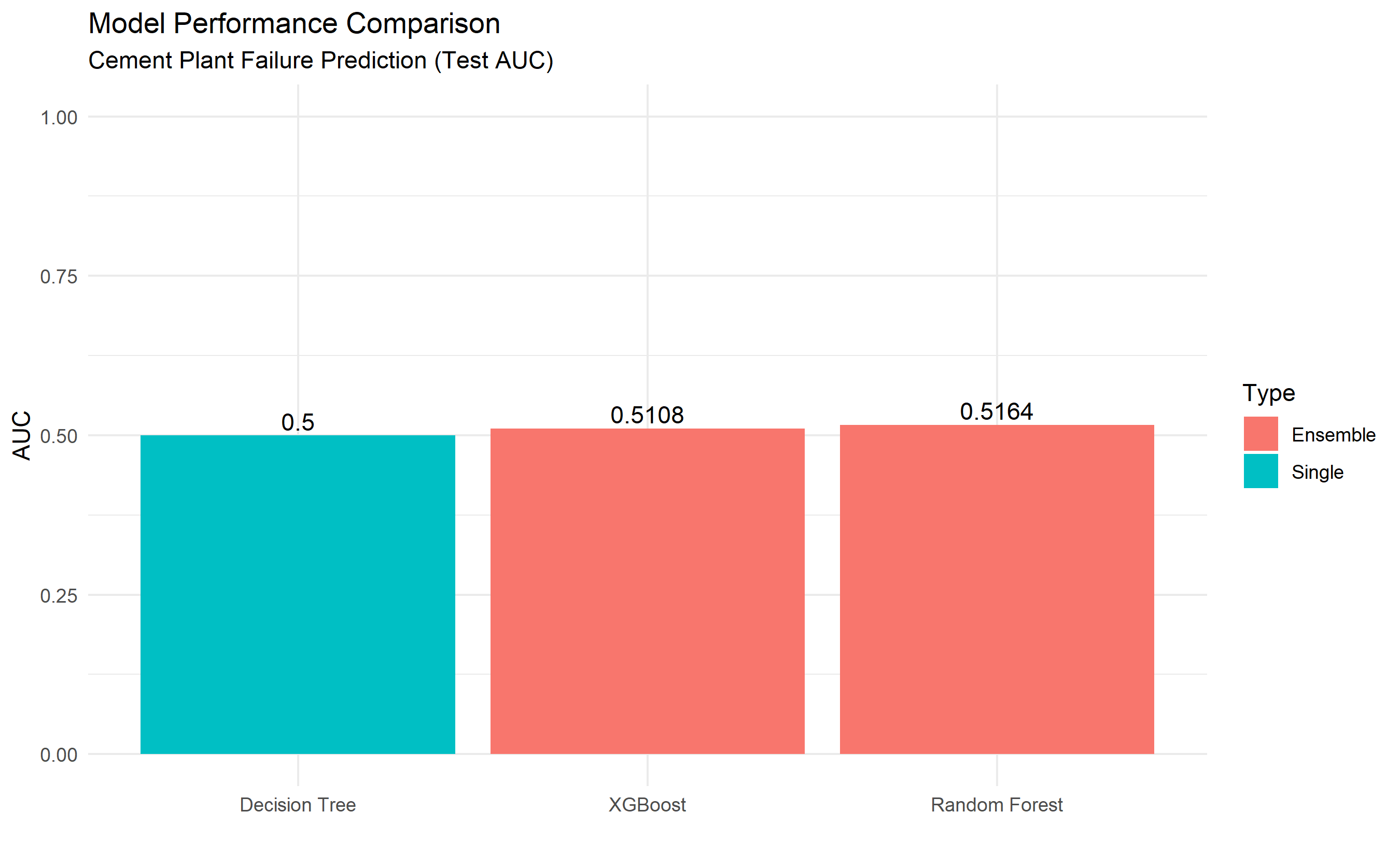
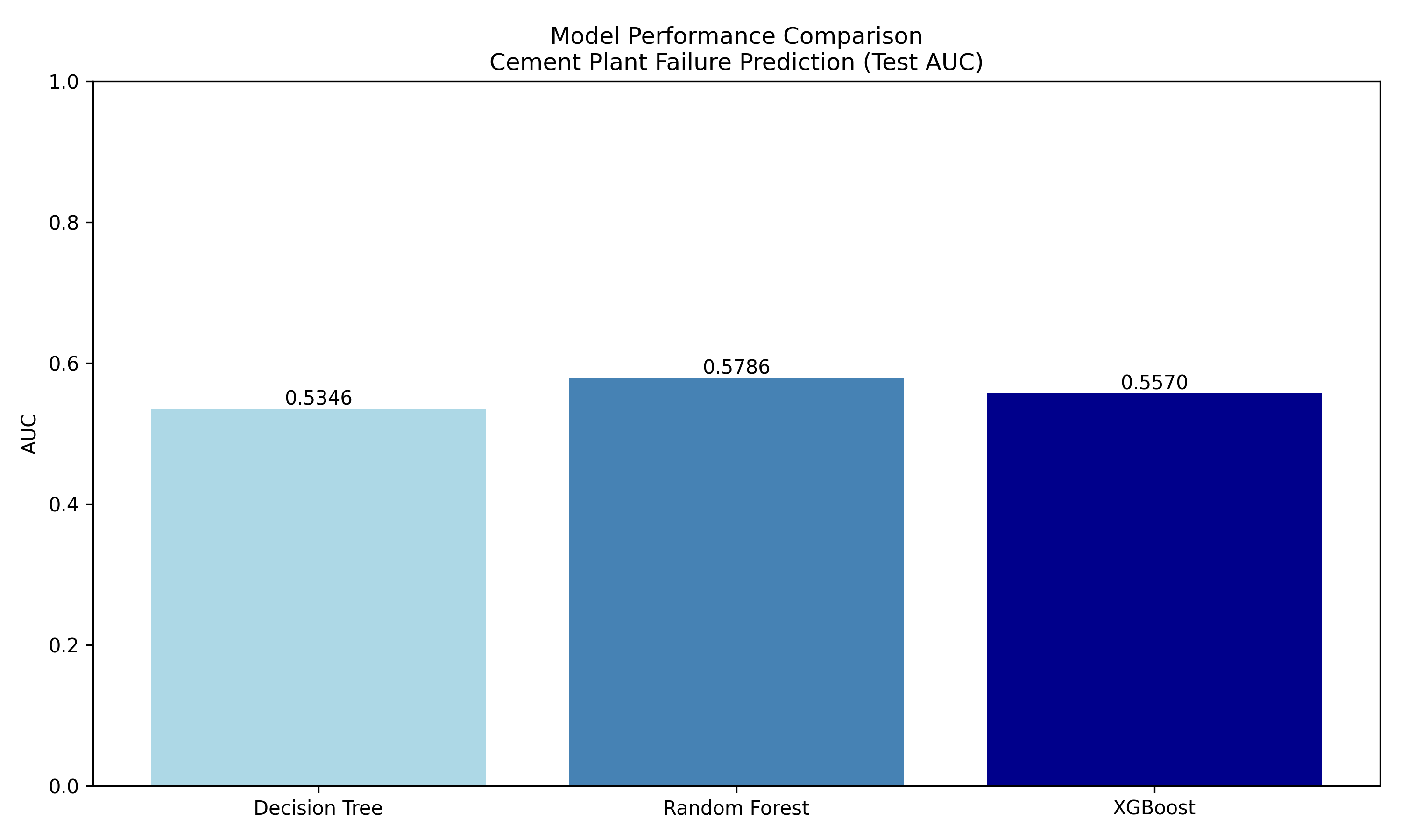
Let’s compare decision tree, Random Forest, and XGBoost on the cement plant dataset.

R

library(tidyverse)
library(rpart)
library(randomForest)
library(xgboost)
library(pROC)

# Prepare data
set.seed(2026)
train_idx <- sample(1:nrow(cement_data), 0.7 * nrow(cement_data))

X_train <- as.matrix(cement_data[train_idx,  c("temperature", "vibration", "power_consumption", "rpm", "pressure", "tool_wear_hours")])
X_test  <- as.matrix(cement_data[-train_idx, c("temperature", "vibration", "power_consumption", "rpm", "pressure", "tool_wear_hours")])
y_train <- as.numeric(cement_data$failure_7d[train_idx]) - 1
y_test <- as.numeric(cement_data$failure_7d[-train_idx]) - 1

# 1. Decision Tree
dt <- rpart(
  failure_7d ~ temperature + vibration + power_consumption + rpm + pressure + tool_wear_hours,
  data = cement_data[train_idx, ],
  method = "class"
)
dt_pred <- predict(dt, cement_data[-train_idx, ], type = "prob")[, 2]
dt_auc <- auc(y_test, dt_pred)

# 2. Random Forest
rf <- randomForest(
  failure_7d ~ temperature + vibration + power_consumption + rpm + pressure + tool_wear_hours,
  data = cement_data[train_idx, ],
  ntree = 200,
  mtry = 2
)
rf_pred <- predict(rf, cement_data[-train_idx, ], type = "prob")[, 2]
rf_auc <- auc(y_test, rf_pred)

# 3. XGBoost
dtrain <- xgb.DMatrix(X_train, label = y_train)
dtest <- xgb.DMatrix(X_test, label = y_test)

xgb_model <- xgb.train(
  params = list(objective = "binary:logistic", eval_metric = "auc",
                eta = 0.05, max_depth = 5, subsample = 0.8),
  data = dtrain,
  nrounds = 100,
  verbose = 0
)
xgb_pred <- predict(xgb_model, dtest)
xgb_auc <- auc(y_test, xgb_pred)

# Compare
comparison <- tibble(
  Model = c("Decision Tree", "Random Forest", "XGBoost"),
  AUC = c(as.numeric(dt_auc), as.numeric(rf_auc), as.numeric(xgb_auc)),
  Type = c("Single", "Ensemble", "Ensemble")
)

cat("Model Comparison:\n")
#> Model Comparison:
print(comparison)
#> # A tibble: 3 × 3
#>   Model           AUC Type    
#>   <chr>         <dbl> <chr>   
#> 1 Decision Tree 0.5   Single  
#> 2 Random Forest 0.516 Ensemble
#> 3 XGBoost       0.511 Ensemble

ggplot(comparison, aes(x = reorder(Model, AUC), y = AUC, fill = Type)) +
  geom_col(show.legend = TRUE) +
  geom_text(aes(label = round(AUC, 4)), vjust = -0.3) +
  ylim(0, 1) +
  labs(title = "Model Performance Comparison",
       subtitle = "Cement Plant Failure Prediction (Test AUC)",
       x = "", y = "AUC") +
  theme_minimal()

Python

from sklearn.tree import DecisionTreeClassifier
from sklearn.ensemble import RandomForestClassifier
from sklearn.metrics import roc_auc_score, auc
import xgboost as xgb

# Prepare data
X_train, X_test, y_train, y_test = train_test_split(
    X, y, test_size=0.3, random_state=2026
)

# 1. Decision Tree
dt = DecisionTreeClassifier(max_depth=5, random_state=2026)
dt.fit(X_train, y_train)
#> DecisionTreeClassifier(max_depth=5, random_state=2026)
dt_pred = dt.predict_proba(X_test)[:, 1]
dt_auc = roc_auc_score(y_test, dt_pred)

# 2. Random Forest
rf = RandomForestClassifier(n_estimators=200, max_features=2, random_state=2026)
rf.fit(X_train, y_train)
#> RandomForestClassifier(max_features=2, n_estimators=200, random_state=2026)
rf_pred = rf.predict_proba(X_test)[:, 1]
rf_auc = roc_auc_score(y_test, rf_pred)

# 3. XGBoost
xgb_model = XGBClassifier(
    n_estimators=100, eta=0.05, max_depth=5, subsample=0.8, random_state=2026
)
xgb_model.fit(X_train, y_train, verbose=False)
#> XGBClassifier(base_score=None, booster=None, callbacks=None,
#>               colsample_bylevel=None, colsample_bynode=None,
#>               colsample_bytree=None, device=None, early_stopping_rounds=None,
#>               enable_categorical=False, eta=0.05, eval_metric=None,
#>               feature_types=None, feature_weights=None, gamma=None,
#>               grow_policy=None, importance_type=None,
#>               interaction_constraints=None, learning_rate=None, max_bin=None,
#>               max_cat_threshold=None, max_cat_to_onehot=None,
#>               max_delta_step=None, max_depth=5, max_leaves=None,
#>               min_child_weight=None, missing=nan, monotone_constraints=None,
#>               multi_strategy=None, n_estimators=100, n_jobs=None, ...)
xgb_pred = xgb_model.predict_proba(X_test)[:, 1]
xgb_auc = roc_auc_score(y_test, xgb_pred)

# Compare
comparison = pd.DataFrame({
    'Model': ['Decision Tree', 'Random Forest', 'XGBoost'],
    'AUC': [dt_auc, rf_auc, xgb_auc],
    'Type': ['Single', 'Ensemble', 'Ensemble']
})

print("Model Comparison:")
#> Model Comparison:
print(comparison)
#>            Model       AUC      Type
#> 0  Decision Tree  0.534623    Single
#> 1  Random Forest  0.578618  Ensemble
#> 2        XGBoost  0.557017  Ensemble

# Plot
fig, ax = plt.subplots(figsize=(10, 6))
bars = ax.bar(comparison['Model'], comparison['AUC'],
              color=['lightblue', 'steelblue', 'darkblue'])
ax.set_ylabel('AUC')
#> Text(0, 0.5, 'AUC')
ax.set_ylim(0, 1)
#> (0.0, 1.0)
ax.set_title('Model Performance Comparison\nCement Plant Failure Prediction (Test AUC)')
#> Text(0.5, 1.0, 'Model Performance Comparison\nCement Plant Failure Prediction (Test AUC)')
for bar in bars:
    height = bar.get_height()
    ax.text(bar.get_x() + bar.get_width()/2., height,
            f'{height:.4f}', ha='center', va='bottom')
#> Text(0.0, 0.5346234826232746, '0.5346')
#> Text(1.0, 0.5786176600556263, '0.5786')
#> Text(2.0, 0.5570169738244392, '0.5570')
plt.tight_layout()
plt.savefig('model_comparison.png', dpi=100, bbox_inches='tight')
plt.show()

Caution📝 Section 15.7 Review Questions

1. Rank the three models by interpretability. Which would you deploy in a regulatory environment?
2. Estimate the computational cost (training time, inference speed) for each model. Which is fastest?
3. If data arrives in batches and you can retrain weekly, which model would you choose?
4. Suggest scenarios where you’d prefer the simpler Decision Tree despite lower AUC.

20.8 Case Study: Predictive Maintenance in a Nigerian Cement Plant

R

# Full pipeline: feature engineering → Random Forest → XGBoost → decision rule

# Step 1: Feature engineering
cement_features <- cement_data |>
  mutate(
    temp_vibration_ratio = temperature / (vibration + 0.1),
    power_per_rpm = power_consumption / (rpm + 1),
    high_wear = ifelse(tool_wear_hours > 4000, 1, 0),
    high_temp = ifelse(temperature > 160, 1, 0),
    high_vibration = ifelse(vibration > 8, 1, 0)
  )

cat("=== PREDICTIVE MAINTENANCE PIPELINE ===\n\n")
#> === PREDICTIVE MAINTENANCE PIPELINE ===

# Step 2: Train Random Forest
set.seed(2026)
train_idx <- sample(1:nrow(cement_features), 0.7 * nrow(cement_features))

rf_full <- randomForest(
  failure_7d ~ temperature + vibration + power_consumption + rpm + pressure +
               tool_wear_hours + high_wear + high_temp + high_vibration,
  data = cement_features[train_idx, ],
  ntree = 200,
  mtry = 3
)

# Step 3: Train XGBoost
X_train_xgb <- as.matrix(cement_features[train_idx,  c("temperature", "vibration", "power_consumption", "rpm", "pressure",
                    "tool_wear_hours", "high_wear", "high_temp", "high_vibration")])
X_test_xgb  <- as.matrix(cement_features[-train_idx, c("temperature", "vibration", "power_consumption", "rpm", "pressure",
                    "tool_wear_hours", "high_wear", "high_temp", "high_vibration")])
y_train_xgb <- as.numeric(cement_features$failure_7d[train_idx]) - 1
y_test_xgb <- as.numeric(cement_features$failure_7d[-train_idx]) - 1

dtrain_xgb <- xgb.DMatrix(X_train_xgb, label = y_train_xgb)
dtest_xgb <- xgb.DMatrix(X_test_xgb, label = y_test_xgb)

xgb_final <- xgb.train(
  params = list(objective = "binary:logistic", eval_metric = "auc",
                eta = 0.05, max_depth = 5, subsample = 0.8),
  data = dtrain_xgb,
  nrounds = 150,
  verbose = 0
)

# Step 4: Model evaluation
rf_pred_test <- predict(rf_full, cement_features[-train_idx, ], type = "prob")[, 2]
xgb_pred_test <- predict(xgb_final, dtest_xgb)

rf_test_auc <- auc(y_test_xgb, rf_pred_test)
xgb_test_auc <- auc(y_test_xgb, xgb_pred_test)

cat("Random Forest Test AUC:", round(as.numeric(rf_test_auc), 4), "\n")
#> Random Forest Test AUC: 0.5244
cat("XGBoost Test AUC:", round(as.numeric(xgb_test_auc), 4), "\n\n")
#> XGBoost Test AUC: 0.5015

# Step 5: Business recommendation
# Define risk tiers based on probability threshold
risk_thresholds <- c(0.3, 0.6)  # Low: <0.3, Medium: 0.3-0.6, High: >0.6

test_data_with_risk <- cement_features[-train_idx, ] |>
  mutate(
    failure_prob = xgb_pred_test,
    risk_tier = case_when(
      failure_prob < 0.3 ~ "Low-risk (Check monthly)",
      failure_prob < 0.6 ~ "Medium-risk (Check weekly)",
      TRUE ~ "High-risk (Daily inspection)"
    )
  )

risk_distribution <- test_data_with_risk |>
  group_by(risk_tier) |>
  summarise(
    n_units = n(),
    actual_failure_rate = mean(as.numeric(failure_7d) - 1),
    avg_failure_prob = mean(failure_prob)
  )

cat("=== MAINTENANCE TRIAGE RESULTS ===\n")
#> === MAINTENANCE TRIAGE RESULTS ===
print(risk_distribution)
#> # A tibble: 2 × 4
#>   risk_tier                  n_units actual_failure_rate avg_failure_prob
#>   <chr>                        <int>               <dbl>            <dbl>
#> 1 Low-risk (Check monthly)       584               0.113           0.0872
#> 2 Medium-risk (Check weekly)      16               0.125           0.376

# Expected maintenance cost
cost_monthly <- 1000       # ₦1,000 per monthly check
cost_weekly <- 3000        # ₦3,000 per weekly check
cost_daily <- 10000        # ₦10,000 per daily inspection

total_cost <- nrow(test_data_with_risk[test_data_with_risk$risk_tier == "Low-risk (Check monthly)", ]) * cost_monthly +
              nrow(test_data_with_risk[test_data_with_risk$risk_tier == "Medium-risk (Check weekly)", ]) * cost_weekly +
              nrow(test_data_with_risk[test_data_with_risk$risk_tier == "High-risk (Daily inspection)", ]) * cost_daily

cat("\n=== BUSINESS IMPACT ===\n")
#> 
#> === BUSINESS IMPACT ===
cat("Total annual maintenance cost: ₦", total_cost * 52, "\n")
#> Total annual maintenance cost: ₦ 32864000
cat("Cost per unit per year: ₦", total_cost * 52 / nrow(test_data_with_risk), "\n")
#> Cost per unit per year: ₦ 54773.33

Python

# Full pipeline with feature engineering

# Step 1: Feature engineering
cement_features = cement_data.copy()
cement_features['temp_vibration_ratio'] = cement_features['temperature'] / (cement_features['vibration'] + 0.1)
cement_features['power_per_rpm'] = cement_features['power_consumption'] / (cement_features['rpm'] + 1)
cement_features['high_wear'] = (cement_features['tool_wear_hours'] > 4000).astype(int)
cement_features['high_temp'] = (cement_features['temperature'] > 160).astype(int)
cement_features['high_vibration'] = (cement_features['vibration'] > 8).astype(int)

print("=== PREDICTIVE MAINTENANCE PIPELINE ===\n")
#> === PREDICTIVE MAINTENANCE PIPELINE ===

# Step 2: Train Random Forest
X_train_full = cement_features[cement_features.index.isin(np.arange(int(0.7*len(cement_features))))][
    ['temperature', 'vibration', 'power_consumption', 'rpm', 'pressure', 'tool_wear_hours',
     'high_wear', 'high_temp', 'high_vibration']
]
y_train_full = cement_features[cement_features.index.isin(np.arange(int(0.7*len(cement_features))))]['failure_7d']

rf_full = RandomForestClassifier(n_estimators=200, max_features=3, random_state=2026)
rf_full.fit(X_train_full, y_train_full)
#> RandomForestClassifier(max_features=3, n_estimators=200, random_state=2026)

# Step 3: Prepare test data
X_test_full = cement_features[~cement_features.index.isin(np.arange(int(0.7*len(cement_features))))][
    ['temperature', 'vibration', 'power_consumption', 'rpm', 'pressure', 'tool_wear_hours',
     'high_wear', 'high_temp', 'high_vibration']
]
y_test_full = cement_features[~cement_features.index.isin(np.arange(int(0.7*len(cement_features))))]['failure_7d']

# Predictions
rf_pred_test = rf_full.predict_proba(X_test_full)[:, 1]
rf_test_auc = roc_auc_score(y_test_full, rf_pred_test)

print(f"Random Forest Test AUC: {rf_test_auc:.4f}\n")
#> Random Forest Test AUC: 0.4796

# Step 4: Define risk tiers
test_data_with_risk = cement_features[~cement_features.index.isin(np.arange(int(0.7*len(cement_features))))].copy()
test_data_with_risk['failure_prob'] = rf_pred_test
test_data_with_risk['risk_tier'] = pd.cut(
    test_data_with_risk['failure_prob'],
    bins=[0, 0.3, 0.6, 1.0],
    labels=['Low-risk (Monthly)', 'Medium-risk (Weekly)', 'High-risk (Daily)']
)

print("=== MAINTENANCE TRIAGE RESULTS ===")
#> === MAINTENANCE TRIAGE RESULTS ===
risk_summary = test_data_with_risk.groupby('risk_tier', observed=True).agg({
    'failure_7d': ['count', 'mean'],
    'failure_prob': 'mean'
}).round(4)
risk_summary.columns = ['n_units', 'actual_failure_rate', 'avg_failure_prob']
print(risk_summary)
#>                       n_units  actual_failure_rate  avg_failure_prob
#> risk_tier                                                           
#> Low-risk (Monthly)        573               0.1082            0.1290
#> Medium-risk (Weekly)       27               0.1111            0.3633

# Cost analysis
costs = {'Low-risk (Monthly)': 1000, 'Medium-risk (Weekly)': 3000, 'High-risk (Daily)': 10000}
test_data_with_risk['maintenance_cost'] = test_data_with_risk['risk_tier'].astype(str).map(costs).astype(float)
annual_cost = test_data_with_risk['maintenance_cost'].sum() * 52

print(f"\n=== BUSINESS IMPACT ===")
#> 
#> === BUSINESS IMPACT ===
print(f"Total annual maintenance cost: ₦{annual_cost:,.0f}")
#> Total annual maintenance cost: ₦34,008,000
print(f"Cost per unit per year: ₦{annual_cost / len(test_data_with_risk):,.0f}")
#> Cost per unit per year: ₦56,680

Caution📝 Section 15.8 Review Questions

1. How would you measure the business impact of the predictive maintenance system?
2. If the high-risk tier causes production delays, how would you adjust the probability thresholds?
3. How often should you retrain the models as new sensor data arrives?
4. What ethical considerations arise when assigning maintenance schedules to different equipment?

20.9 Chapter 15 Exercises

1. Bootstrap variance: Implement bootstrap sampling from scratch. Verify that ~63% of samples appear in each bootstrap sample.

2. Bagging reduction: Train a single decision tree and a bagging ensemble on the same data. Compare train vs. test error. Does bagging reduce variance?

3. Feature subsampling effect: Train Random Forests with different max_features values (1, √p, p/2, p). Plot OOB error vs. max_features.

4. Learning curve analysis: Plot train and test error vs. number of trees (n_estimators). At what point does the test error plateau?

5. Hyperparameter sensitivity: Use grid search to find the best learning rate and max_depth for XGBoost. Visualize the grid search results as a heatmap.

6. Early stopping demonstration: Train XGBoost with and without early stopping. Compare final test error and number of rounds.

7. Feature importance comparison: Train Random Forest and XGBoost on the same data. Compare their feature importance rankings. Are they consistent?

8. Prediction calibration: For XGBoost, check if predicted probabilities match actual success rates. Use a calibration plot.

9. Imbalanced data: Reweight the cement plant data to increase failure class weight. Does this improve AUC on the minority class?

10. Case study extension: Deploy the predictive maintenance system to a second cement plant (different synthetic data). Retrain and compare performance.

20.10 Further Reading

1. Schapire, R. E., & Freund, Y. (2012). Boosting: Foundations and Algorithms. MIT Press. — Theoretical foundations of boosting.

2. Friedman, J. H. (2001). “Greedy function approximation: a gradient boosting machine.” Annals of Statistics, 29(5), 1189–1232. — Original gradient boosting paper.

3. Chen, T., & Guestrin, C. (2016). “XGBoost: A scalable tree boosting system.” KDD, 785–794. — XGBoost paper.

4. Ke, G., Meng, Q., et al. (2017). “LightGBM: A fast, distributed, high-performance gradient boosting framework.” NIPS, 3149–3157. — LightGBM paper.

5. James, G., Witten, D., Hastie, T., & Tibshirani, R. (2013). An Introduction to Statistical Learning. Springer. — Accessible chapter on bagging and boosting.

20.11 Chapter 15 Appendix

20.11.1 A. Proof: OOB Error ≈ k-Fold CV Error

Theorem: For large B (number of bootstrap samples), the out-of-bag error of a bagging ensemble is approximately equal to k-fold cross-validation error.

Proof Sketch:

1. For each sample i, the fraction of bootstrap samples that exclude it is approximately \((1 - 1/n)^n \approx e^{-1} \approx 0.368\) (about 37%).

2. For large B, roughly B × 0.37 trees have sample i in their OOB set.

3. The OOB error for sample i uses only trees trained without i, analogous to leave-one-out CV.

4. Averaging over all n samples gives OOB error, which approximates LOO-CV error.

5. LOO-CV error is a lower-variance estimate of k-fold CV error; they converge as B → ∞.

20.11.2 B. Derivation of Gradient Boosting Update

Objective: Minimize loss L(y, f(x)) over B iterations.

Gradient descent in function space:

At iteration m, we want to move in the direction that reduces loss:

\[f_m(x) = f_{m-1}(x) + \Delta f_m(x)\]

where \(\Delta f_m\) is chosen to maximize the negative gradient:

\[\Delta f_m(x) = -\eta \cdot \nabla_f L(y, f(x))|_{f=f_{m-1}}\]

For regression (squared loss):

\[\nabla L = \frac{\partial}{\partial f} \frac{1}{2}(y - f)^2 = -(y - f)\]

So the residual is the negative gradient:

\[r_i = y_i - f_{m-1}(x_i)\]

We fit \(tree_m\) to \((X, r)\) and update:

\[f_m(x) = f_{m-1}(x) + \eta \cdot tree_m(x)\]

For classification (log loss):

\[\nabla L = \frac{\partial}{\partial f} \log(1 + e^{-yf}) = \frac{-y}{1 + e^{yf}}\]

This is more complex but follows the same principle: fit trees to gradients and update.

20.11.3 C. Permutation Importance Formula

Permutation importance measures the drop in model performance when a feature’s values are randomly shuffled (breaking the relationship between feature and target).

\[PI(X_j) = \frac{1}{B} \sum_{b=1}^{B} \left[ Acc(X_b, y) - Acc(X_b^{-j}, y) \right]\]

where: - \(X_b\) is feature matrix for tree b with feature j unshuffled. - \(X_b^{-j}\) is feature matrix with feature j values randomly shuffled. - \(Acc\) is model accuracy (or any metric).

Advantages over impurity-based importance: - Not biased towards high-cardinality features. - Accounts for feature interactions. - Works for any model, not just trees.

---

End of Chapter 15