---
title: "Regularised Regression and Feature Selection"
---
```{python}
#| label: python-setup-10-regularised-regression
#| include: false
import numpy as np
import pandas as pd
import matplotlib.pyplot as plt
import seaborn as sns
from sklearn.linear_model import Ridge, RidgeCV, LinearRegression
from sklearn.preprocessing import StandardScaler
from sklearn.model_selection import cross_val_score
from sklearn.linear_model import Lasso, LassoCV
from sklearn.linear_model import ElasticNetCV
from sklearn.linear_model import LassoCV
from sklearn.model_selection import cross_validate
from sklearn.feature_selection import RFE
from sklearn.linear_model import LinearRegression
from sklearn.linear_model import LogisticRegression, LogisticRegressionCV
from sklearn.model_selection import train_test_split
from sklearn.metrics import roc_auc_score, roc_curve, accuracy_score
```
::: {.callout-note icon="false"}
## 📋 Learning Objectives
By the end of this chapter, you will be able to:
- Understand the bias-variance trade-off and the overfitting problem
- Apply Ridge regression (L2 regularisation) to stabilise coefficients
- Apply Lasso regression (L1 regularisation) for automatic feature selection
- Combine Ridge and Lasso via Elastic Net
- Use cross-validation to select the optimal regularisation parameter
- Perform automated feature selection using forward, backward, and recursive methods
- Diagnose and prevent overfitting in real-world applications
:::
## The Overfitting Problem
Imagine you are studying for an examination. You have access to five years of past exam papers. One approach: memorise every past question and its answer. You ace the practice papers with a perfect score. Then the real exam arrives with slightly different questions — and you flounder, because you memorised the past papers instead of understanding the underlying concepts.
This is exactly what **overfitting** means in machine learning. A model that has memorised its training data can reproduce training examples with near-perfect accuracy, but it has not learned the true underlying pattern — it has learned the noise, the quirks, the idiosyncrasies of that particular dataset. When new data arrives that it has never seen before, the model fails because the noise in the training data does not appear in the new data.
Here is a concrete business example. A bank wants to predict which customers will default on a personal loan. They have 1,000 training records and a junior data scientist who adds 50 features to the model — income, age, credit score, number of transactions, days since last deposit, and 45 other variables. The model fits the training data beautifully, with 98% accuracy. Excited, the bank deploys it. Six months later, the actual default rate on customers the model marked as "safe" is far higher than expected. The model had learned that customer number 487 defaulted AND lived near Ikorodu AND had exactly 12 transactions in March — a coincidence specific to the training data that does not predict anything about future customers.
The solution is **regularisation**: a mathematical technique that deliberately prevents the model from fitting the training data too perfectly. By adding a penalty for complexity, regularisation forces the model to find simpler, more general patterns — patterns that are more likely to hold when new data arrives.
### The Bias-Variance Trade-off: Finding the Sweet Spot
Understanding regularisation requires understanding a fundamental tension at the heart of statistics called the **bias-variance trade-off**. To grasp this intuitively, think of an archery competition.
An archer with **high bias** always shoots to the left of the target. Their arrows are consistently wrong in the same direction — they have a systematic error. The bow might be miscalibrated. In modelling terms, a high-bias model is too simple: it misses real patterns because it cannot represent them. A linear model fitted to data that is genuinely curved will always underestimate at the extremes and overestimate in the middle — a systematic, consistent error.
An archer with **high variance** is inconsistent: sometimes they shoot left, sometimes right, sometimes high, sometimes low. Their arrows are scattered unpredictably across the target. In modelling terms, a high-variance model changes dramatically when retrained on slightly different data. It is too sensitive to the specific sample it was trained on. A model with 50 features fitted to 100 data points is in this territory — small changes in which 100 points you happened to sample could lead to wildly different coefficient estimates.
The ideal archer is both accurate (low bias) and consistent (low variance). The ideal model hits the bull's-eye reliably. But here is the cruel reality: **as you make a model more complex (adding more features, adding interaction terms, using higher-degree polynomials), bias goes down but variance goes up**. A complex model fits the training data better, but it becomes more sensitive to noise. Regularisation is the tool that tames this trade-off — it deliberately increases bias slightly to massively reduce variance, resulting in a model that generalises better to new data.
Every estimator's total prediction error can be decomposed as:
**Total error = Bias² + Variance + Irreducible error**
The irreducible error is the noise in the data that no model can ever eliminate — the fundamental randomness in outcomes. The goal of regularisation is to minimise bias² + variance together, even though reducing one tends to increase the other.
::: {.callout-note icon="false"}
## 📘 Theory: Learning Curves and Regularisation
**Training error:** Error on the data used to fit the model; decreases with model complexity
**Test (generalisation) error:** Error on held-out data; initially decreases, then increases (the "U-shape")
**Overfitting signal:** Training error << Test error
Regularisation adds a penalty to the objective function, discouraging extreme coefficient values and encouraging simpler models. This trades a small increase in bias for a larger reduction in variance, shifting the bias-variance optimum toward lower complexity.
:::
::: {.callout-caution icon="false"}
## 📝 Section 10.1 Review Questions
1. Draw the typical U-shaped learning curve showing training and test error. Label the overfitting region.
2. If a model has very high training R² but low test R², what is the likely problem?
3. Explain: "Regularisation introduces bias to reduce variance." Is this always desirable?
4. In a high-dimensional problem (p >> n), why is regularisation essential?
:::
## Ridge Regression (L2 Regularisation)
**Ridge regression** adds an L2 penalty (sum of squared coefficients) to the OLS objective, shrinking coefficients toward zero without eliminating any.
::: {.callout-note icon="false"}
## 📘 Theory: Ridge Objective and Solution
Ridge minimises:
$$S_{\text{Ridge}}(\beta) = \sum_{i=1}^{n} (y_i - \beta_0 - \sum_{j=1}^{p} \beta_j x_{ij})^2 + \lambda \sum_{j=1}^{p} \beta_j^2$$
The second term is the L2 penalty, controlled by **λ** (lambda), the regularisation parameter:
- λ = 0: OLS (no penalty)
- λ → ∞: all coefficients → 0
**Closed-form solution:**
$$\hat{\boldsymbol{\beta}}_{\text{Ridge}} = (\mathbf{X}^T \mathbf{X} + \lambda \mathbf{I})^{-1} \mathbf{X}^T \mathbf{y}$$
The added λI term makes the matrix inversion stable even when $\mathbf{X}^T \mathbf{X}$ is near-singular (multicollinearity).
:::
::: {.callout-tip icon="false"}
## 🔑 Key Formula: Ridge Regression
$$\hat{\boldsymbol{\beta}}_{\text{Ridge}} = (\mathbf{X}^T \mathbf{X} + \lambda \mathbf{I})^{-1} \mathbf{X}^T \mathbf{y}$$
**Properties:**
- Coefficients are never exactly zero (shrinkage, but not elimination)
- Symmetric shrinkage: larger coefficients shrink more in absolute value
- λ controls the amount of shrinkage
- More interpretable than OLS when multicollinearity is severe
:::
### Choosing λ via Cross-Validation
The optimal λ is found by K-fold cross-validation:
1. Fit Ridge with a sequence of λ values (e.g., λ ∈ {0.01, 0.1, 1, 10, 100})
2. For each λ, compute average CV error across k folds
3. Select λ with lowest CV error
4. Refit on full data with this λ
### Worked Example: Ridge for Nigerian SME Credit Data
::: {.panel-tabset}
## R
```{r}
library(glmnet)
library(tidyverse)
set.seed(42)
n <- 300
# Synthetic Nigerian SME credit data: 20 correlated financial ratios
# Features: debt-to-equity, leverage, ROA, profitability, liquidity, etc.
X_raw <- matrix(rnorm(n * 20, mean = 0, sd = 1), nrow = n, ncol = 20)
# Add multicollinearity: each variable is partly a linear combination of others
for (j in 1:20) {
if (j > 1) {
X_raw[, j] <- 0.7 * X_raw[, j] + 0.3 * X_raw[, j - 1] + rnorm(n, 0, 0.2)
}
}
# Outcome: credit amount (thousands NGN)
y <- 100 + 15 * X_raw[, 1] + 12 * X_raw[, 2] - 8 * X_raw[, 5] + rnorm(n, 0, 30)
y <- pmax(y, 0)
colnames(X_raw) <- paste0("Ratio_", 1:20)
# Standardise features (required for glmnet)
X_scaled <- scale(X_raw)
# Fit Ridge with range of λ
ridge_fit <- glmnet(X_scaled, y, alpha = 0, lambda = 10^seq(3, -2, length = 100))
# Cross-validation to find optimal λ
ridge_cv <- cv.glmnet(X_scaled, y, alpha = 0, nfolds = 5)
cat("Cross-Validation Results for Ridge Regression:\n\n")
cat("Optimal λ (minimum CV error):", round(ridge_cv$lambda.min, 4), "\n")
cat("λ (one standard error rule):", round(ridge_cv$lambda.1se, 4), "\n")
cat("Minimum CV MSE:", round(min(ridge_cv$cvm), 2), "\n\n")
# Coefficients at optimal λ
coef_ridge <- coef(ridge_fit, s = ridge_cv$lambda.min)[-1] # exclude intercept
cat("Ridge coefficients (at λ =", round(ridge_cv$lambda.min, 4), "):\n")
print(round(coef_ridge, 3))
# Compare with OLS
fit_ols <- lm(y ~ X_scaled)
coef_ols <- coef(fit_ols)[-1]
# Visualise coefficient paths
# Use line = 4 to push titles above glmnet's top-axis variable-count annotation
par(mfrow = c(1, 2), mar = c(5, 5, 5, 1), oma = c(0, 0, 2, 0))
plot(ridge_cv, main = "")
title(main = "Cross-Validation Error", line = 4)
abline(v = log(ridge_cv$lambda.min), col = "red", lty = 2, lwd = 2)
plot(ridge_fit, xvar = "lambda", main = "")
title(main = "Coefficient Paths", line = 4)
abline(v = log(ridge_cv$lambda.min), col = "red", lty = 2, lwd = 2)
mtext("Ridge Regression", outer = TRUE, cex = 1.2, font = 2)
par(mfrow = c(1, 1), oma = c(0, 0, 0, 0))
# Comparison: OLS vs Ridge coefficients
comparison <- tibble(
Variable = colnames(X_scaled),
OLS = coef_ols,
Ridge = coef_ridge,
Ratio = Ridge / OLS
)
cat("\n\nComparison of OLS vs Ridge Coefficients:\n")
print(comparison |> arrange(desc(abs(OLS))) |> head(10))
# Performance: OLS vs Ridge on training data
pred_ols <- predict(fit_ols, newdata = data.frame(X_scaled))
pred_ridge <- predict(ridge_fit, newx = X_scaled, s = ridge_cv$lambda.min)
rmse_ols <- sqrt(mean((y - pred_ols)^2))
rmse_ridge <- sqrt(mean((y - pred_ridge)^2))
cat("\n\nTraining RMSE:\n")
cat("OLS: ", round(rmse_ols, 2), "\n")
cat("Ridge:", round(rmse_ridge, 2), "\n")
# Cross-validation RMSE
cv_rmse_ridge <- ridge_cv$cvm[which.min(ridge_cv$cvm)]
cat("Ridge CV RMSE:", round(sqrt(cv_rmse_ridge), 2), "\n")
```
## Python
```{python}
import numpy as np
import pandas as pd
import matplotlib.pyplot as plt
from sklearn.linear_model import Ridge, RidgeCV, LinearRegression
from sklearn.preprocessing import StandardScaler
from sklearn.model_selection import cross_val_score

np.random.seed(42)
n = 300

# Generate correlated financial ratios
X_raw = np.random.normal(0, 1, (n, 20))
for j in range(1, 20):
    X_raw[:, j] = 0.7 * X_raw[:, j] + 0.3 * X_raw[:, j - 1] + np.random.normal(0, 0.2, n)

# Outcome
y = 100 + 15 * X_raw[:, 0] + 12 * X_raw[:, 1] - 8 * X_raw[:, 4] + np.random.normal(0, 30, n)
y = np.maximum(y, 0)

# Standardise
scaler = StandardScaler()
X_scaled = scaler.fit_transform(X_raw)

# Find optimal λ via cross-validation
alphas = np.logspace(-2, 3, 100)
ridge_cv = RidgeCV(alphas=alphas, cv=5)
ridge_cv.fit(X_scaled, y)
print(f"Cross-Validation Results for Ridge Regression:\n")
print(f"Optimal α (λ): {ridge_cv.alpha_:.4f}")
print(f"CV score (R²): {ridge_cv.score(X_scaled, y):.4f}\n")
# Fit Ridge at optimal α
ridge_final = Ridge(alpha=ridge_cv.alpha_)
ridge_final.fit(X_scaled, y)
# OLS for comparison
ols = LinearRegression()
ols.fit(X_scaled, y)
# Coefficients
coef_ridge = ridge_final.coef_
coef_ols = ols.coef_
# Create comparison dataframe
comparison = pd.DataFrame({
'Variable': [f'Ratio_{i+1}' for i in range(20)],
'OLS': coef_ols,
'Ridge': coef_ridge
})
comparison['Shrinkage'] = 1 - (comparison['Ridge'] / comparison['OLS']).abs()
print("Comparison of OLS vs Ridge Coefficients (top 10 by OLS magnitude):")
print(comparison.sort_values('OLS', key=abs, ascending=False).head(10).to_string(index=False))
# Plot coefficient paths
fig, axes = plt.subplots(1, 2, figsize=(14, 5))
# Plot 1: Coefficient shrinkage
ax = axes[0]
x_pos = np.arange(20)
ax.scatter(x_pos, coef_ols, alpha=0.7, s=80, label='OLS', color='steelblue')
ax.scatter(x_pos, coef_ridge, alpha=0.7, s=80, label=f'Ridge (α={ridge_cv.alpha_:.3f})', color='darkred')
for i in range(20):
ax.plot([i, i], [coef_ols[i], coef_ridge[i]], 'k--', alpha=0.3, linewidth=0.5)
ax.set_xlabel('Feature Index', fontsize=11)
ax.set_ylabel('Coefficient Value', fontsize=11)
ax.set_title('OLS vs Ridge: Coefficient Shrinkage', fontsize=12, fontweight='bold')
ax.legend()
ax.grid(True, alpha=0.3)
# Plot 2: Coefficient magnitude comparison
ax = axes[1]
ax.scatter(np.abs(coef_ols), np.abs(coef_ridge), alpha=0.7, s=80, color='steelblue')
ax.plot([0, np.abs(coef_ols).max()], [0, np.abs(coef_ols).max()], 'k--', linewidth=1, alpha=0.5)
ax.set_xlabel('|OLS coefficient|', fontsize=11)
ax.set_ylabel('|Ridge coefficient|', fontsize=11)
ax.set_title('Magnitude of Coefficients: OLS vs Ridge', fontsize=12, fontweight='bold')
ax.grid(True, alpha=0.3)
plt.tight_layout()
plt.savefig('ridge_vs_ols.png', dpi=300, bbox_inches='tight')
plt.show()
# Cross-validation RMSE
ols_cv_scores = cross_val_score(LinearRegression(), X_scaled, y, cv=5, scoring='neg_mean_squared_error')
ridge_cv_scores = cross_val_score(Ridge(alpha=ridge_cv.alpha_), X_scaled, y, cv=5, scoring='neg_mean_squared_error')
ols_cv_rmse = np.sqrt(-ols_cv_scores.mean())
ridge_cv_rmse = np.sqrt(-ridge_cv_scores.mean())
print(f"\n\nCross-Validation RMSE:")
print(f"OLS: {ols_cv_rmse:.2f}")
print(f"Ridge: {ridge_cv_rmse:.2f}")
```
:::
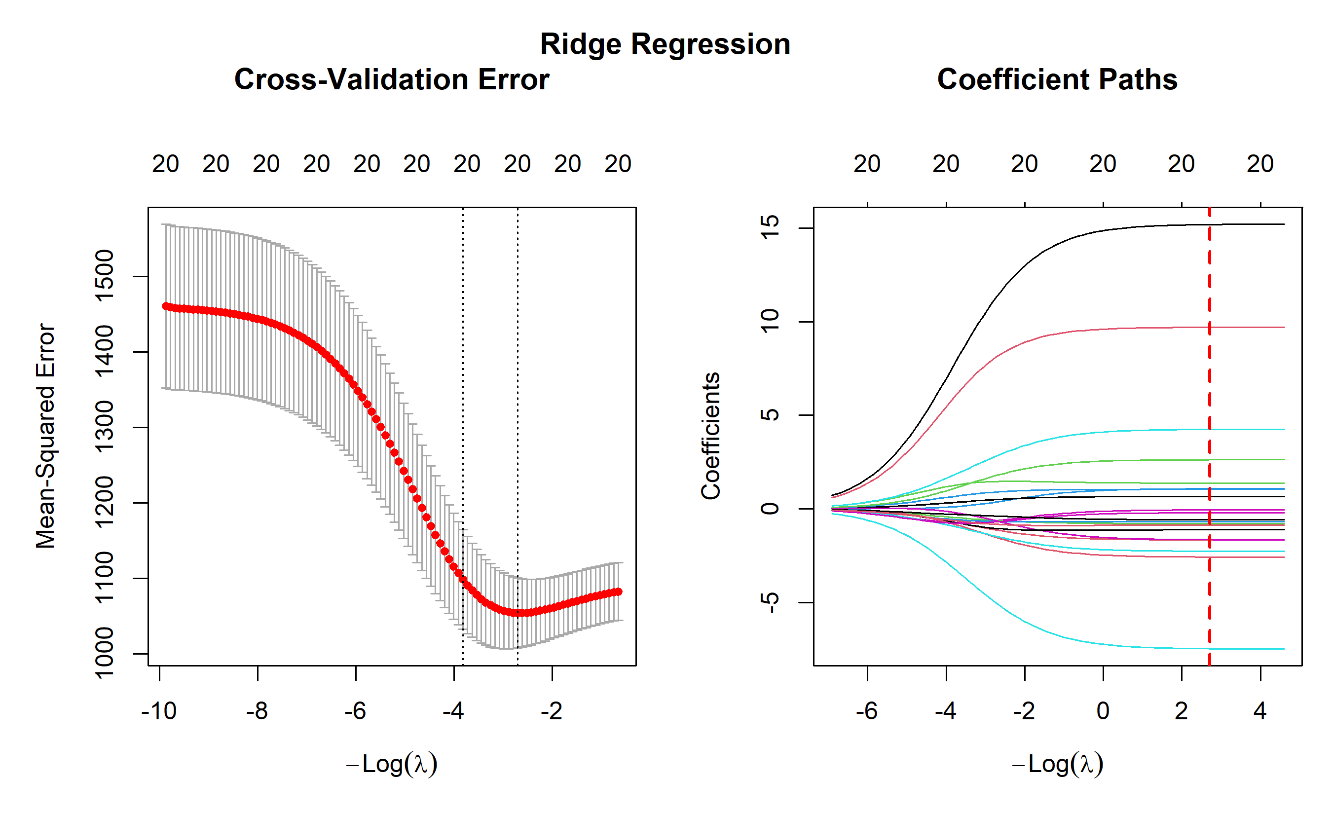
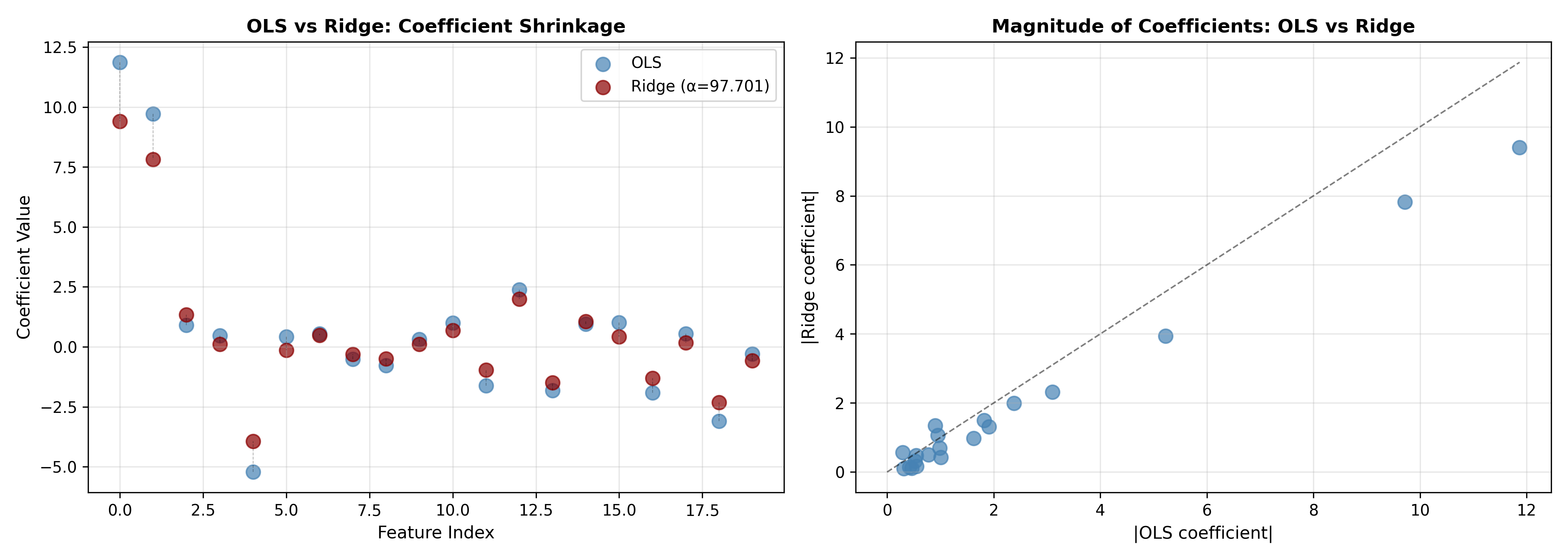
**Key insights:**
- Ridge shrinks all coefficients toward zero, with larger coefficients shrinking more
- The optimal λ balances fit and complexity
- Ridge is more stable than OLS when features are correlated
- All features are retained; none is eliminated
::: {.callout-caution icon="false"}
## 📝 Section 10.2 Review Questions
1. Why does Ridge add a penalty on β² rather than |β|?
2. If λ = 0, Ridge reduces to OLS. If λ is very large, what happens to coefficients?
3. In the Nigerian SME example, why might Ridge perform better than OLS on new loan applications?
4. What is the trade-off between using a smaller vs larger λ?
:::
## Lasso Regression (L1 Regularisation)
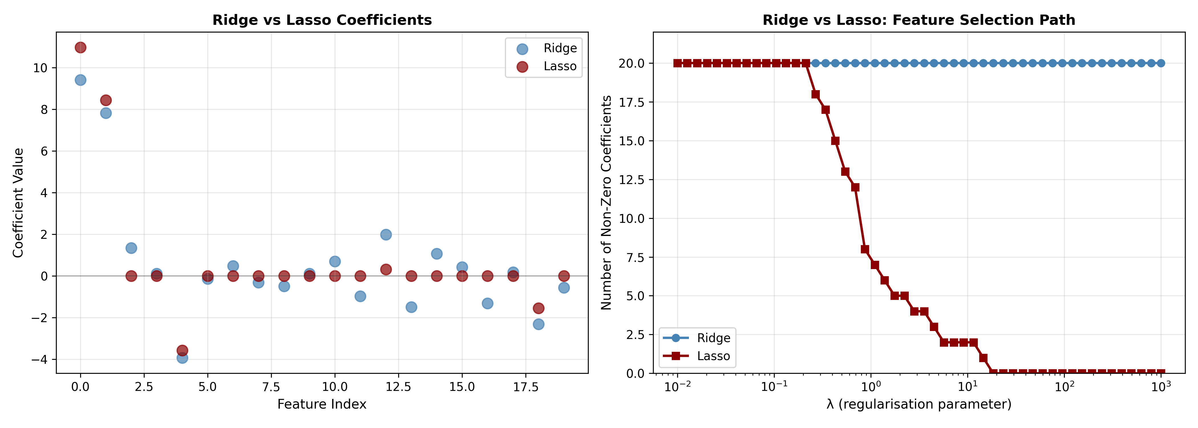
**Lasso (Least Absolute Shrinkage and Selection Operator)** adds an L1 penalty (sum of absolute coefficients), which can shrink coefficients **exactly to zero**, providing automatic feature selection.
::: {.callout-note icon="false"}
## 📘 Theory: Lasso Objective
Lasso minimises:
$$S_{\text{Lasso}}(\beta) = \sum_{i=1}^{n} (y_i - \beta_0 - \sum_{j=1}^{p} \beta_j x_{ij})^2 + \lambda \sum_{j=1}^{p} |\beta_j|$$
Unlike Ridge, there is no closed-form solution. The solution is found via **coordinate descent**, updating one coefficient at a time while holding others fixed.
**Soft-thresholding:** For a univariate problem, the Lasso solution has a simple form:
$$\hat{\beta}_{\text{Lasso}} = \text{sign}(\hat{\beta}_{\text{OLS}}) \max(|\hat{\beta}_{\text{OLS}}| - \lambda, 0)$$
- If |β̂_OLS| ≤ λ, then β̂_Lasso = 0 (coefficient is eliminated)
- If |β̂_OLS| > λ, then β̂_Lasso = β̂_OLS − λ · sign(β̂_OLS) (coefficient is shrunk)
:::
::: {.callout-tip icon="false"}
## 🔑 Key Formula: Lasso Objective and Sparsity
$$S_{\text{Lasso}}(\beta) = \text{RSS} + \lambda \sum_{j=1}^{p} |\beta_j|$$
**Why Lasso produces sparsity (geometric intuition):**
In Ridge, the penalty is an ellipse (β₁² + β₂² = c), which smoothly touches the contours of the objective. In Lasso, the penalty is a diamond (|β₁| + |β₂| = c), whose corners coincide with the axes (β_j = 0). Thus, the optimum often occurs at a corner, setting some coefficients exactly to zero.
:::
### Ridge vs Lasso: When to Use Which
| Aspect | Ridge | Lasso |
|---|---|---|
| **Penalty** | L2 (β²) | L1 (\|β\|) |
| **Feature selection** | Shrinks all, eliminates none | Shrinks and eliminates |
| **Use case** | Many relevant predictors, moderate correlation | Want a sparse model, high-dimensional data |
| **Interpretation** | All features retained; harder to explain | Only non-zero features matter; easier to explain |
| **Computation** | Fast (closed form) | Slower (iterative, but still polynomial) |
### Worked Example: Lasso for Feature Selection
::: {.panel-tabset}
## R
```{r}
# Lasso regression with automatic feature selection
# Use same data as Ridge example
# Fit Lasso with range of λ
lasso_fit <- glmnet(X_scaled, y, alpha = 1, lambda = 10^seq(3, -2, length = 100))
# Cross-validation
lasso_cv <- cv.glmnet(X_scaled, y, alpha = 1, nfolds = 5)
cat("Cross-Validation Results for Lasso Regression:\n\n")
cat("Optimal λ (minimum CV error):", round(lasso_cv$lambda.min, 4), "\n")
cat("λ (one standard error rule):", round(lasso_cv$lambda.1se, 4), "\n")
cat("Number of non-zero coefficients at λ_min:", sum(coef(lasso_fit, s = lasso_cv$lambda.min) != 0) - 1, "\n")
cat("Number of non-zero coefficients at λ_1se:", sum(coef(lasso_fit, s = lasso_cv$lambda.1se) != 0) - 1, "\n\n")
# Coefficients at both λ values
coef_lasso_min <- coef(lasso_fit, s = lasso_cv$lambda.min)[-1]
coef_lasso_1se <- coef(lasso_fit, s = lasso_cv$lambda.1se)[-1]
cat("Selected features (λ_min):\n")
selected_min <- which(coef_lasso_min != 0)
if (length(selected_min) > 0) {
for (j in selected_min) {
cat(sprintf(" Ratio_%d: %.3f\n", j, coef_lasso_min[j]))
}
} else {
cat(" (none)\n")
}
cat("\nSelected features (λ_1se):\n")
selected_1se <- which(coef_lasso_1se != 0)
if (length(selected_1se) > 0) {
for (j in selected_1se) {
cat(sprintf(" Ratio_%d: %.3f\n", j, coef_lasso_1se[j]))
}
} else {
cat(" (none)\n")
}
# Visualise
par(mfrow = c(1, 2), mar = c(5, 5, 3, 1))
# Plot 1: CV curve
plot(lasso_cv, main = "Lasso Regression: Cross-Validation")
abline(v = log(lasso_cv$lambda.min), col = "red", lty = 2, lwd = 2)
abline(v = log(lasso_cv$lambda.1se), col = "orange", lty = 2, lwd = 2)
legend("topleft", legend = c("λ_min", "λ_1se"),
col = c("red", "orange"), lty = 2, lwd = 2)
# Plot 2: Coefficient path (showing sparsity)
plot(lasso_fit, xvar = "lambda", main = "Lasso Regression: Coefficient Path (Sparsity)")
abline(v = log(lasso_cv$lambda.min), col = "red", lty = 2, lwd = 2)
abline(v = log(lasso_cv$lambda.1se), col = "orange", lty = 2, lwd = 2)
par(mfrow = c(1, 1))
# Compare Ridge and Lasso
cat("\n\nComparison of Ridge vs Lasso (coefficient paths):\n\n")
ridge_cv <- cv.glmnet(X_scaled, y, alpha = 0, nfolds = 5)
coef_ridge_opt <- coef(ridge_fit, s = ridge_cv$lambda.min)[-1]
comparison_rl <- tibble(
Variable = colnames(X_scaled),
Ridge = coef_ridge_opt,
Lasso_min = coef_lasso_min,
Lasso_1se = coef_lasso_1se
)
cat("Features with non-zero Lasso coefficients:\n")
print(comparison_rl |> filter(Lasso_min != 0 | Lasso_1se != 0) |>
arrange(desc(abs(Lasso_min))))
# Visualization: Ridge vs Lasso paths
par(mfrow = c(1, 2), mar = c(5, 5, 3, 1))
plot(ridge_fit, xvar = "lambda", main = "Ridge: All coefficients retained")
abline(v = log(ridge_cv$lambda.min), col = "blue", lty = 2, lwd = 2)
plot(lasso_fit, xvar = "lambda", main = "Lasso: Sparse solution (some coefficients zero)")
abline(v = log(lasso_cv$lambda.min), col = "red", lty = 2, lwd = 2)
par(mfrow = c(1, 1))
```
## Python
```{python}
from sklearn.linear_model import Lasso, LassoCV
import numpy as np

# Fit Lasso with cross-validation
alphas = np.logspace(-2, 3, 100)
lasso_cv = LassoCV(alphas=alphas, cv=5, max_iter=10000)
lasso_cv.fit(X_scaled, y)
print(f"Cross-Validation Results for Lasso Regression:\n")
print(f"Optimal α (λ): {lasso_cv.alpha_:.4f}")
print(f"Number of non-zero coefficients: {np.sum(lasso_cv.coef_ != 0)}\n")
# Selected features
coef_lasso = lasso_cv.coef_
selected_features = np.where(coef_lasso != 0)[0]
print(f"Selected features (non-zero Lasso coefficients):")
for j in selected_features:
print(f" Ratio_{j+1}: {coef_lasso[j]:.4f}")
if len(selected_features) == 0:
print(" (all coefficients shrunk to zero)")
# Compare Ridge and Lasso
fig, axes = plt.subplots(1, 2, figsize=(14, 5))
# Plot 1: Coefficient comparison
ax = axes[0]
x_pos = np.arange(20)
ax.scatter(x_pos, coef_ridge, alpha=0.7, s=80, label='Ridge', color='steelblue')
ax.scatter(x_pos, coef_lasso, alpha=0.7, s=80, label='Lasso', color='darkred')
ax.axhline(y=0, color='black', linestyle='-', linewidth=0.5, alpha=0.5)
ax.set_xlabel('Feature Index', fontsize=11)
ax.set_ylabel('Coefficient Value', fontsize=11)
ax.set_title('Ridge vs Lasso Coefficients', fontsize=12, fontweight='bold')
ax.legend()
ax.grid(True, alpha=0.3)
# Plot 2: Number of non-zero coefficients
ax = axes[1]
lambda_seq = np.logspace(-2, 3, 50)
ridge_nonzero = np.full(len(lambda_seq), 20) # Ridge never zeros out
lasso_nonzero = []
for lam in lambda_seq:
lasso_temp = Lasso(alpha=lam, max_iter=10000)
lasso_temp.fit(X_scaled, y)
lasso_nonzero.append(np.sum(lasso_temp.coef_ != 0))
ax.semilogx(lambda_seq, ridge_nonzero, 'o-', label='Ridge', color='steelblue', linewidth=2)
ax.semilogx(lambda_seq, lasso_nonzero, 's-', label='Lasso', color='darkred', linewidth=2)
ax.set_xlabel('λ (regularisation parameter)', fontsize=11)
ax.set_ylabel('Number of Non-Zero Coefficients', fontsize=11)
ax.set_title('Ridge vs Lasso: Feature Selection Path', fontsize=12, fontweight='bold')
ax.legend()
ax.grid(True, alpha=0.3)
ax.set_ylim([0, 22])
plt.tight_layout()
plt.savefig('ridge_vs_lasso.png', dpi=300, bbox_inches='tight')
plt.show()
print(f"\n\nLasso Sparse Solution:")
print(f"Features eliminated: {np.sum(coef_lasso == 0)} out of 20")
print(f"Features retained: {np.sum(coef_lasso != 0)} out of 20")
```
:::
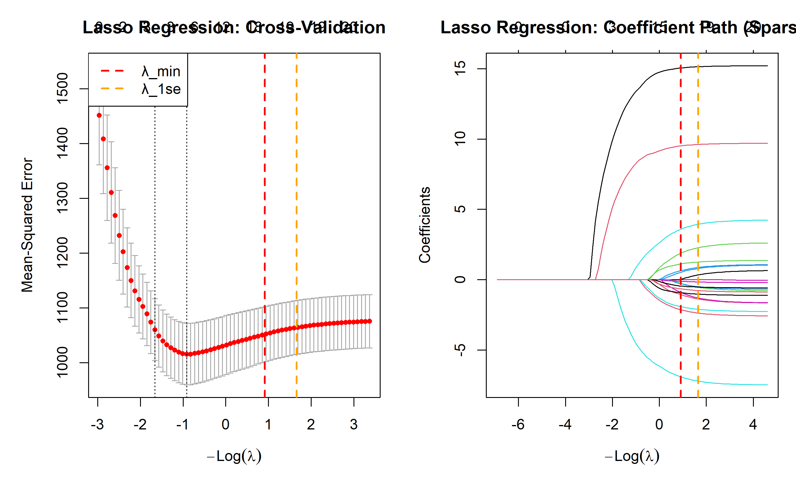
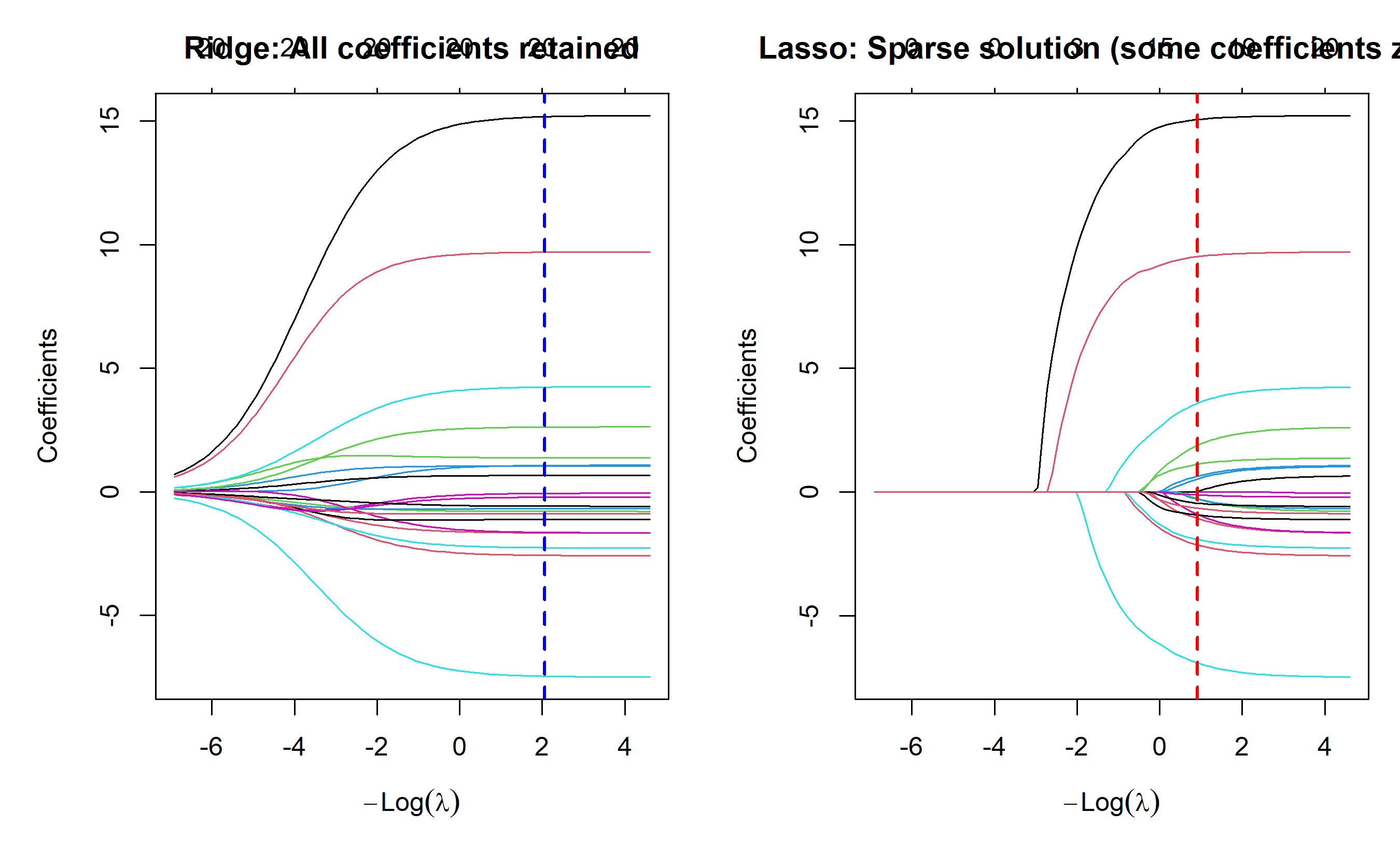
**Key insight:** At λ_1se (one standard error rule), Lasso selects only a handful of true drivers, dramatically simplifying the model while maintaining predictive accuracy.
::: {.callout-caution icon="false"}
## 📝 Section 10.3 Review Questions
1. Why does the Lasso objective's diamond-shaped constraint produce sparsity, while Ridge's ellipse does not?
2. In the SME credit example, suppose Lasso selects only Ratio_1 and Ratio_2. How would you use this for business decisions?
3. Compare interpretation difficulty: Ridge (all features) vs Lasso (sparse features).
4. Can Lasso with a given λ select more features than Ridge with the same λ? Explain.
:::
## Elastic Net: Combining L1 and L2
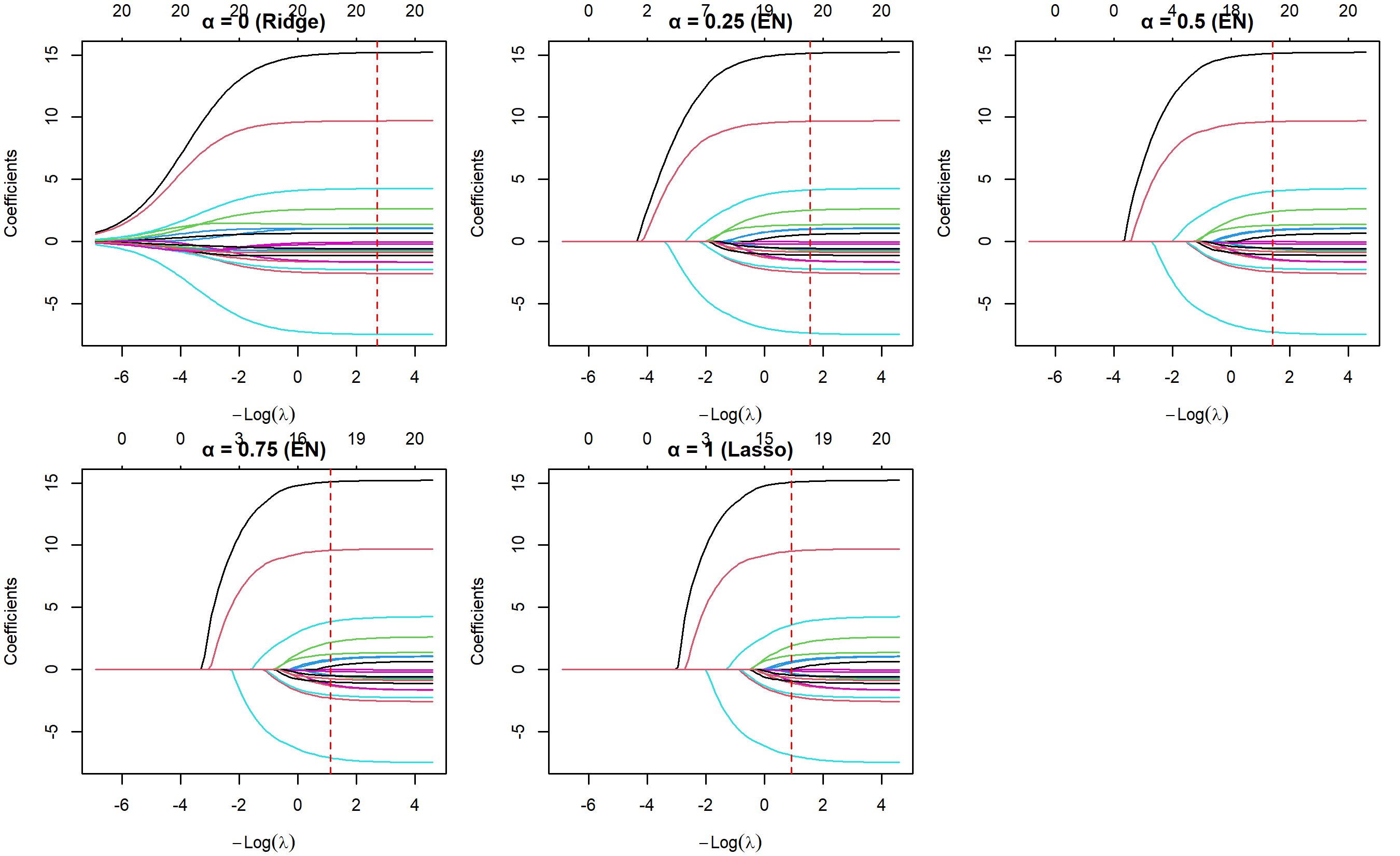
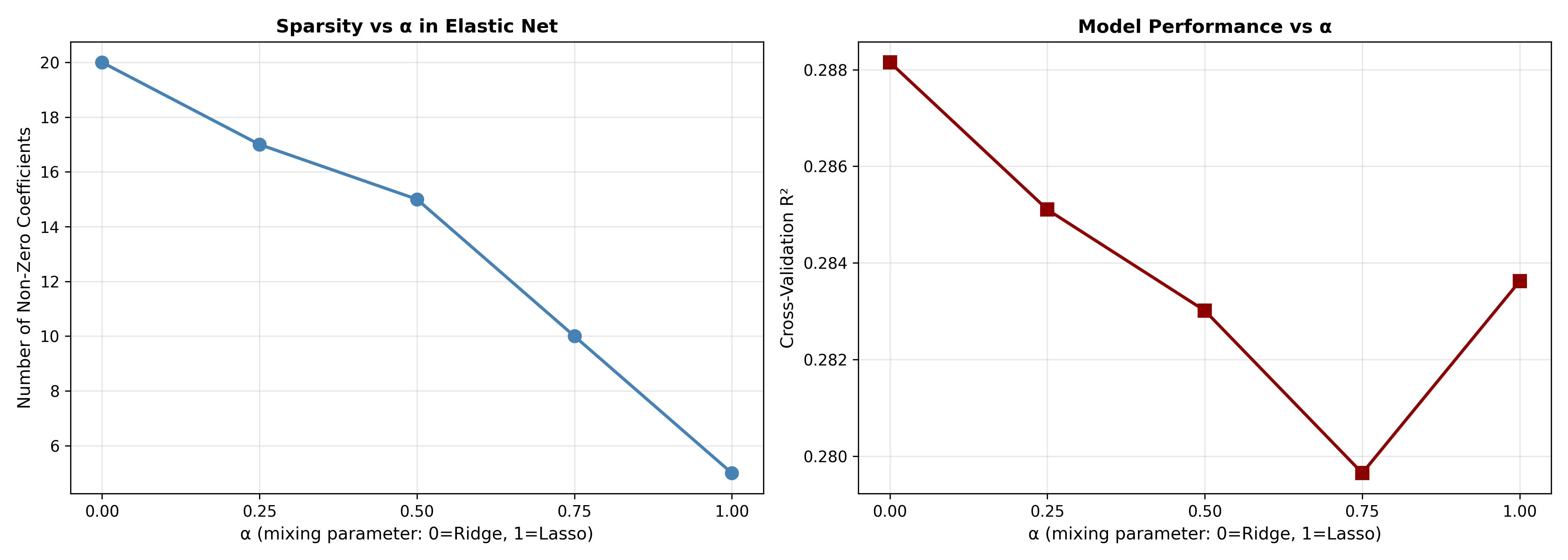
**Elastic Net** combines Ridge (L2) and Lasso (L1) penalties, capturing benefits of both.
::: {.callout-note icon="false"}
## 📘 Theory: Elastic Net Objective
$$S_{\text{EN}}(\beta) = \sum_{i=1}^{n} (y_i - \beta_0 - \sum_{j} \beta_j x_{ij})^2 + \lambda \left[ (1 - \alpha) \frac{1}{2} \sum_{j} \beta_j^2 + \alpha \sum_{j} |\beta_j| \right]$$
where:
- α ∈ [0, 1] is the mixing parameter
- α = 0: Ridge
- α = 1: Lasso
- α ∈ (0, 1): combination of both
**When Elastic Net excels:**
1. **Grouping effect:** If several features are correlated and relevant, Lasso may arbitrarily select one. Elastic Net's L2 component encourages all to be included together.
2. **High-dimensional data:** When p >> n, Elastic Net is more stable than pure Lasso.
3. **Unknown feature relationships:** When you don't know if features are important individually or as groups, Elastic Net hedges bets.
:::
::: {.callout-tip icon="false"}
## 🔑 Key Formula: Elastic Net
$$S_{\text{EN}}(\beta) = \text{RSS} + \lambda \left[ (1 - \alpha) \frac{||β||_2^2}{2} + \alpha ||β||_1 \right]$$
**Intuition:**
- L2 component: shrinks all coefficients, encourages grouping of correlated predictors
- L1 component: performs feature selection, sets some coefficients to zero
- Balance via α: tune based on domain knowledge or CV
:::
### Worked Example: Elastic Net
::: {.panel-tabset}
## R
```{r}
# Elastic Net with varying α (mixing parameter)
# Fit Elastic Net models with different α values
en_models <- list()
en_cv_results <- list()
alpha_values <- c(0, 0.25, 0.5, 0.75, 1)
for (alpha_val in alpha_values) {
fit <- glmnet(X_scaled, y, alpha = alpha_val, lambda = 10^seq(3, -2, length = 100))
fit_cv <- cv.glmnet(X_scaled, y, alpha = alpha_val, nfolds = 5)
en_models[[as.character(alpha_val)]] <- fit
en_cv_results[[as.character(alpha_val)]] <- fit_cv
}
cat("Elastic Net: Model Comparison Across α values\n\n")
comparison_en <- tibble(
Alpha = alpha_values,
Method = c("Ridge", "EN (0.25)", "EN (0.5)", "EN (0.75)", "Lasso"),
Lambda_min = sapply(en_cv_results, function(x) x$lambda.min),
CV_MSE = sapply(en_cv_results, function(x) min(x$cvm)),
Nonzero_coefs = sapply(alpha_values, function(a) {
sum(coef(en_models[[as.character(a)]], s = en_cv_results[[as.character(a)]]$lambda.min) != 0) - 1
})
)
print(comparison_en)
# Visualise coefficient paths for different α
par(mfrow = c(2, 3), mar = c(4, 4, 2, 1))
method_labels <- c("Ridge", "EN", "EN", "EN", "Lasso")
for (i in seq_along(alpha_values)) {
alpha_val <- alpha_values[i]
plot(en_models[[as.character(alpha_val)]], xvar = "lambda",
main = sprintf("α = %s (%s)", alpha_val, method_labels[i]))
abline(v = log(en_cv_results[[as.character(alpha_val)]]$lambda.min),
col = "red", lty = 2, lwd = 1)
}
par(mfrow = c(1, 1))
cat("\n\nOptimal models by α:\n")
for (alpha_val in alpha_values) {
cv_result <- en_cv_results[[as.character(alpha_val)]]
coefs <- coef(en_models[[as.character(alpha_val)]], s = cv_result$lambda.min)[-1]
nonzero <- sum(coefs != 0)
cat(sprintf("α = %s: λ = %.4f, Non-zero coefficients = %d\n",
alpha_val, cv_result$lambda.min, nonzero))
}
```
## Python
```{python}
from sklearn.linear_model import ElasticNetCV
import numpy as np

# Elastic Net with varying α
alpha_values = [0, 0.25, 0.5, 0.75, 1]
l1_ratios = alpha_values  # α in ElasticNetCV is the l1_ratio

en_models = {}
en_results = []

for l1_ratio in l1_ratios:
    en_cv = ElasticNetCV(l1_ratio=l1_ratio, alphas=np.logspace(-2, 3, 100), cv=5, max_iter=10000)
    en_cv.fit(X_scaled, y)
    en_models[l1_ratio] = en_cv

    en_results.append({
        'Alpha (L1 ratio)': l1_ratio,
        'Method': ['Ridge', 'EN (0.25)', 'EN (0.5)', 'EN (0.75)', 'Lasso'][int(l1_ratio * 4)],
        'Lambda': en_cv.alpha_,
        'CV R²': en_cv.score(X_scaled, y),
        'Non-zero coefs': np.sum(en_cv.coef_ != 0)
    })
en_comparison = pd.DataFrame(en_results)
print("Elastic Net: Model Comparison Across α values\n")
print(en_comparison.to_string(index=False))
# Visualise sparsity vs α
fig, axes = plt.subplots(1, 2, figsize=(14, 5))
# Plot 1: Non-zero coefficients vs α
ax = axes[0]
nonzero_counts = [np.sum(en_models[lr].coef_ != 0) for lr in l1_ratios]
ax.plot(alpha_values, nonzero_counts, 'o-', linewidth=2, markersize=8, color='steelblue')
ax.set_xlabel('α (mixing parameter: 0=Ridge, 1=Lasso)', fontsize=11)
ax.set_ylabel('Number of Non-Zero Coefficients', fontsize=11)
ax.set_title('Sparsity vs α in Elastic Net', fontsize=12, fontweight='bold')
ax.set_xticks(alpha_values)
ax.grid(True, alpha=0.3)
# Plot 2: CV score vs α
ax = axes[1]
cv_scores = [en_models[lr].score(X_scaled, y) for lr in l1_ratios]
ax.plot(alpha_values, cv_scores, 's-', linewidth=2, markersize=8, color='darkred')
ax.set_xlabel('α (mixing parameter: 0=Ridge, 1=Lasso)', fontsize=11)
ax.set_ylabel('Cross-Validation R²', fontsize=11)
ax.set_title('Model Performance vs α', fontsize=12, fontweight='bold')
ax.set_xticks(alpha_values)
ax.grid(True, alpha=0.3)
plt.tight_layout()
plt.savefig('elasticnet_comparison.png', dpi=300, bbox_inches='tight')
plt.show()
print(f"\n\nInterpretation:")
for l1_ratio in l1_ratios:
coef = en_models[l1_ratio].coef_
nonzero = np.sum(coef != 0)
method = ['Ridge', 'EN', 'EN', 'EN', 'Lasso'][int(l1_ratio * 4)]
print(f"{method} (α={l1_ratio}): {nonzero} features selected, R² = {en_models[l1_ratio].score(X_scaled, y):.4f}")
```
:::
::: {.callout-caution icon="false"}
## 📝 Section 10.4 Review Questions
1. When would you choose α = 0.5 over pure Ridge or pure Lasso?
2. If your data has many correlated features and you want a sparse solution, why might Elastic Net (α ≈ 0.7) outperform Lasso?
3. How would you select α: via grid search or prior knowledge?
:::
## Choosing the Penalty: Cross-Validation
The regularisation parameter λ (and α in Elastic Net) must be selected using cross-validation, not by minimising training error.
### The One-Standard-Error Rule
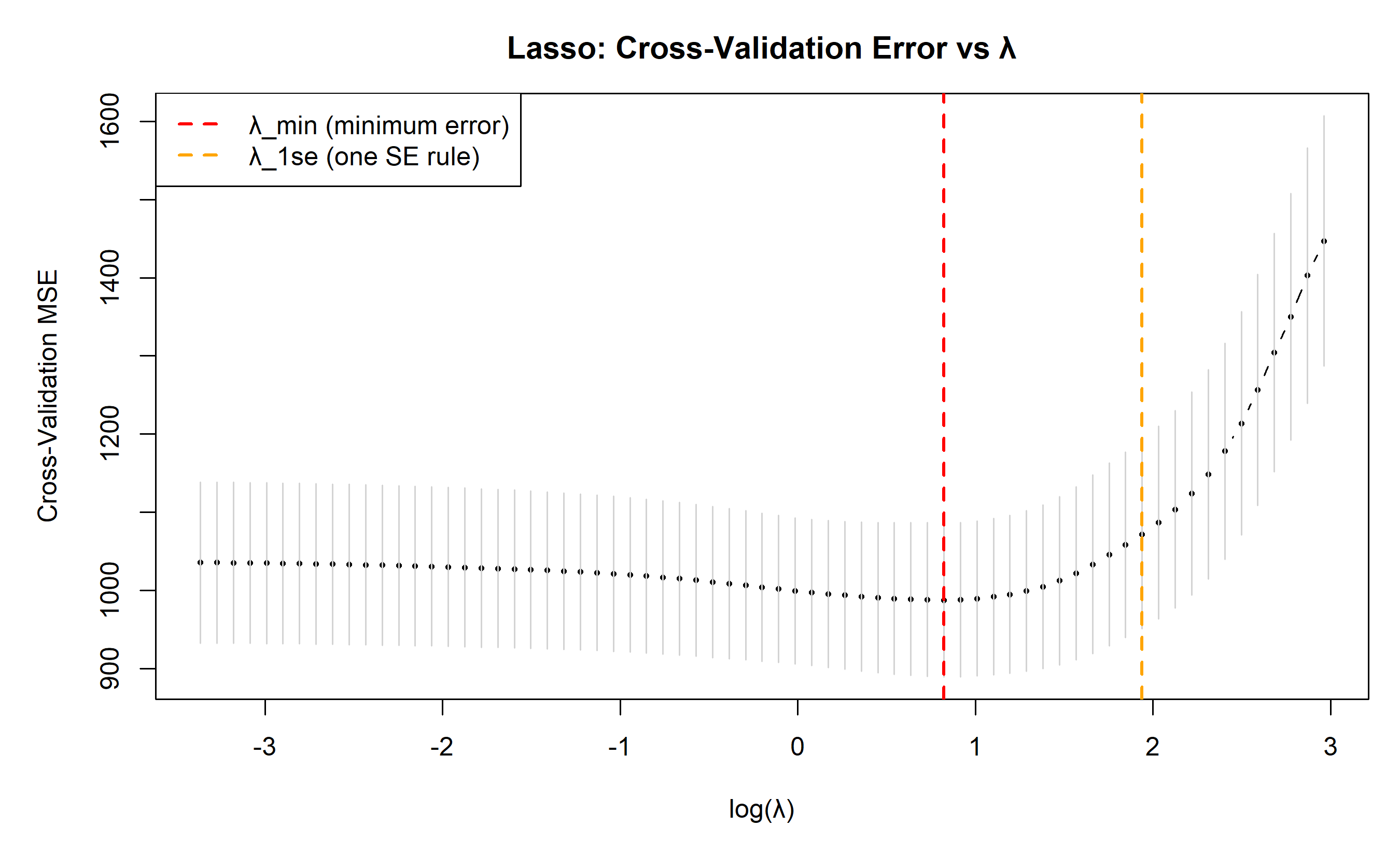
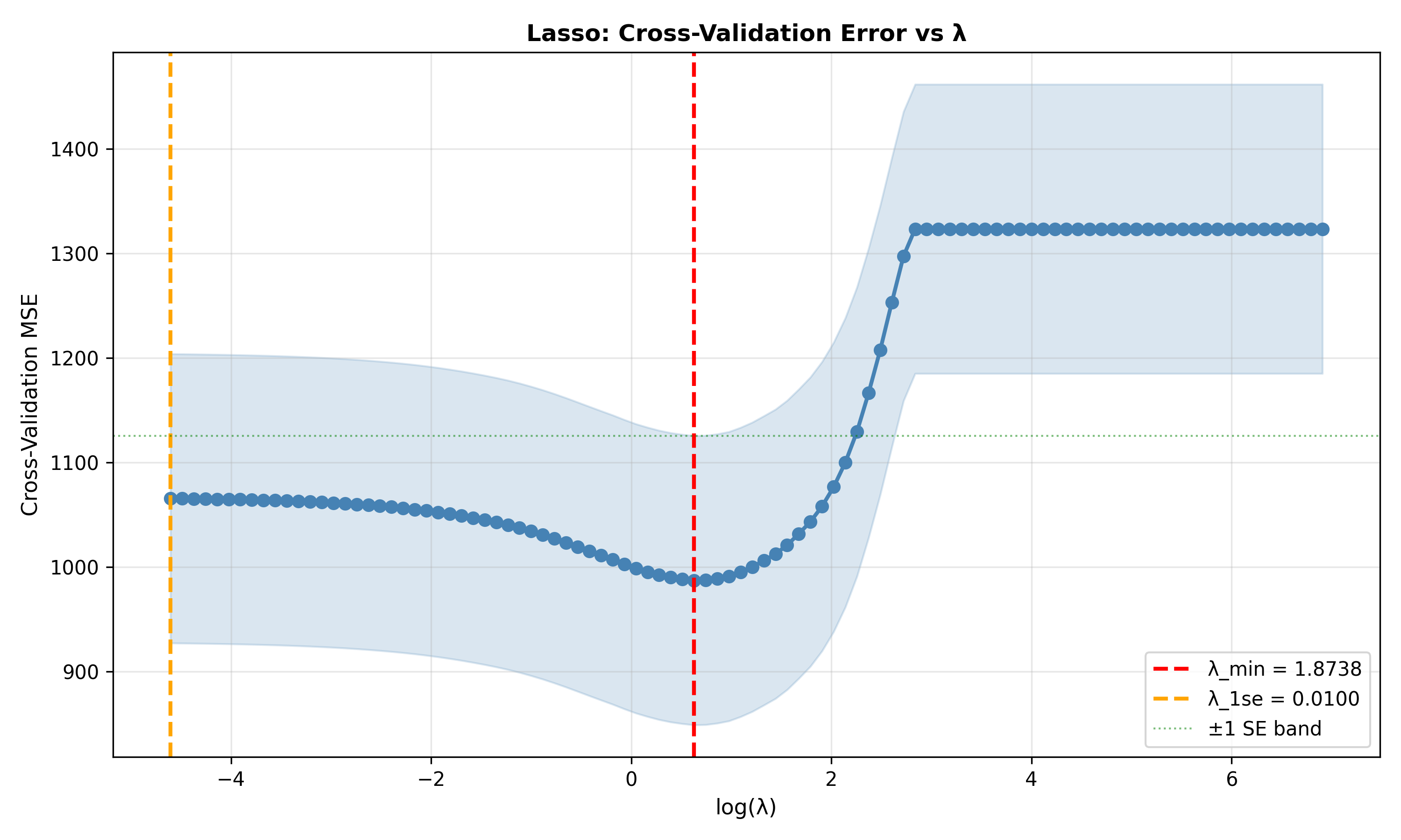
When CV error curves are flat near the minimum, the **one-standard-error rule** suggests:
1. Find λ with minimum CV error: λ_min
2. Find the simplest model within one SE of λ_min: λ_1se
3. Use λ_1se for parsimony (fewer non-zero coefficients, similar accuracy)
::: {.callout-note icon="false"}
## 📘 Theory: Cross-Validation for Regularisation
**K-Fold CV procedure:**
1. Randomly divide data into k equal folds
2. For each fold i = 1, ..., k:
- Leave fold i out (test set)
- Fit model on remaining k−1 folds (training set)
- Compute error on fold i
3. Average error across k folds: CV error
4. Repeat for each λ in a sequence
5. Choose λ that minimises CV error (or λ_1se for parsimony)
**Why this works:** CV error estimates generalisation error on truly held-out data, avoiding overfitting.
:::
### Worked Example: CV Grid Search
::: {.panel-tabset}
## R
```{r}
# Comprehensive CV for hyperparameter tuning

# Already computed above, but let's visualise the full grid

# Lasso CV with detailed output
lasso_cv_full <- cv.glmnet(X_scaled, y, alpha = 1, nfolds = 5, nlambda = 100)

# Extract CV results
lambda_seq <- lasso_cv_full$lambda
cv_mean <- lasso_cv_full$cvm
cv_sd <- lasso_cv_full$cvsd

# Plot with confidence bands
par(mar = c(5, 5, 3, 1))

plot(log(lambda_seq), cv_mean, type = "b", pch = 16, cex = 0.5,
     xlab = "log(λ)", ylab = "Cross-Validation MSE",
     main = "Lasso: Cross-Validation Error vs λ",
     ylim = range(cv_mean - cv_sd, cv_mean + cv_sd))

# Add confidence band
segments(log(lambda_seq), cv_mean - cv_sd, log(lambda_seq), cv_mean + cv_sd, col = "lightgray")

# Mark λ_min and λ_1se
abline(v = log(lasso_cv_full$lambda.min), col = "red", lty = 2, lwd = 2, label = "λ_min")
abline(v = log(lasso_cv_full$lambda.1se), col = "orange", lty = 2, lwd = 2, label = "λ_1se")

legend("topleft", legend = c("λ_min (minimum error)", "λ_1se (one SE rule)"),
       col = c("red", "orange"), lty = 2, lwd = 2)
# Summary
cat("Cross-Validation Summary (Lasso):\n\n")
cat("λ_min =", round(lasso_cv_full$lambda.min, 4), "\n")
cat("CV error at λ_min =", round(min(lasso_cv_full$cvm), 2), "\n")
cat("Number of non-zero coefs at λ_min =", sum(coef(lasso_cv_full, s = "lambda.min") != 0) - 1, "\n\n")
cat("λ_1se =", round(lasso_cv_full$lambda.1se, 4), "\n")
cat("CV error at λ_1se =", round(lasso_cv_full$cvm[lasso_cv_full$lambda == lasso_cv_full$lambda.1se], 2), "\n")
cat("Number of non-zero coefs at λ_1se =", sum(coef(lasso_cv_full, s = "lambda.1se") != 0) - 1, "\n")
# Recommendation
cat("\n\nRecommendation:\n")
cat("For predictive accuracy: use λ_min\n")
cat("For interpretability and sparsity: use λ_1se\n")
```
## Python
```{python}
# Detailed CV analysis with plotting

# Refit Lasso with detailed CV
from sklearn.linear_model import LassoCV

lasso_cv_full = LassoCV(alphas=np.logspace(-2, 3, 100), cv=5, max_iter=10000)
lasso_cv_full.fit(X_scaled, y)
# Extract alphas and CV scores
# Let's compute manually using cross_val_score
from sklearn.model_selection import cross_validate
# Create array of alphas
alphas_manual = np.logspace(-2, 3, 100)
cv_scores_manual = []
for alpha in alphas_manual:
lasso_temp = Lasso(alpha=alpha, max_iter=10000)
cv_scores = -cross_val_score(lasso_temp, X_scaled, y, cv=5, scoring='neg_mean_squared_error')
cv_scores_manual.append(cv_scores.mean())
cv_scores_manual = np.array(cv_scores_manual)
# Find λ_min and λ_1se
min_idx = np.argmin(cv_scores_manual)
lambda_min = alphas_manual[min_idx]
min_score = cv_scores_manual[min_idx]
# One standard error rule
cv_std_manual = np.std(cv_scores_manual)
threshold = min_score + cv_std_manual
idx_1se = np.where(cv_scores_manual <= threshold)[0][0]
lambda_1se = alphas_manual[idx_1se]
print(f"Cross-Validation Summary (Lasso):\n")
print(f"λ_min = {lambda_min:.4f}")
print(f"CV error at λ_min = {min_score:.2f}")
lasso_min = Lasso(alpha=lambda_min, max_iter=10000)
lasso_min.fit(X_scaled, y)
nonzero_min = np.sum(lasso_min.coef_ != 0)
print(f"Number of non-zero coefs at λ_min = {nonzero_min}\n")
print(f"λ_1se = {lambda_1se:.4f}")
lasso_1se = Lasso(alpha=lambda_1se, max_iter=10000)
lasso_1se.fit(X_scaled, y)
nonzero_1se = np.sum(lasso_1se.coef_ != 0)
print(f"CV error at λ_1se = {cv_scores_manual[idx_1se]:.2f}")
print(f"Number of non-zero coefs at λ_1se = {nonzero_1se}")
# Plot
fig, ax = plt.subplots(figsize=(10, 6))
ax.plot(np.log(alphas_manual), cv_scores_manual, 'o-', linewidth=2, markersize=6, color='steelblue')
ax.fill_between(np.log(alphas_manual),
cv_scores_manual - cv_std_manual,
cv_scores_manual + cv_std_manual,
alpha=0.2, color='steelblue')
ax.axvline(np.log(lambda_min), color='red', linestyle='--', linewidth=2, label=f'λ_min = {lambda_min:.4f}')
ax.axvline(np.log(lambda_1se), color='orange', linestyle='--', linewidth=2, label=f'λ_1se = {lambda_1se:.4f}')
ax.axhline(min_score + cv_std_manual, color='green', linestyle=':', linewidth=1, alpha=0.5, label='±1 SE band')
ax.set_xlabel('log(λ)', fontsize=11)
ax.set_ylabel('Cross-Validation MSE', fontsize=11)
ax.set_title('Lasso: Cross-Validation Error vs λ', fontsize=12, fontweight='bold')
ax.legend(fontsize=10)
ax.grid(True, alpha=0.3)
plt.tight_layout()
plt.savefig('cv_lambda_selection.png', dpi=300, bbox_inches='tight')
plt.show()
print(f"\n\nRecommendation:")
print(f"For predictive accuracy: use λ_min = {lambda_min:.4f} ({nonzero_min} features)")
print(f"For interpretability: use λ_1se = {lambda_1se:.4f} ({nonzero_1se} features)")
```
:::
::: {.callout-caution icon="false"}
## 📝 Section 10.5 Review Questions
1. Why do we use cross-validation to select λ, rather than minimising training error?
2. Explain the one-standard-error rule. Why is it useful?
3. If the CV error curve is flat, does the choice of λ matter?
:::
## Automated Feature Selection
Beyond regularisation, several automated methods select important features.
::: {.callout-note icon="false"}
## 📘 Theory: Feature Selection Methods
1. **Forward stepwise selection:**
- Start with no predictors
- At each step, add the predictor that most improves model fit
- Continue until stopping rule (e.g., BIC increase, p-value threshold)
- Fast but greedy (local optimum)
2. **Backward elimination:**
- Start with all predictors
- Remove the least important predictor at each step
- Stop when all remaining predictors are significant
- Often better than forward, but slower
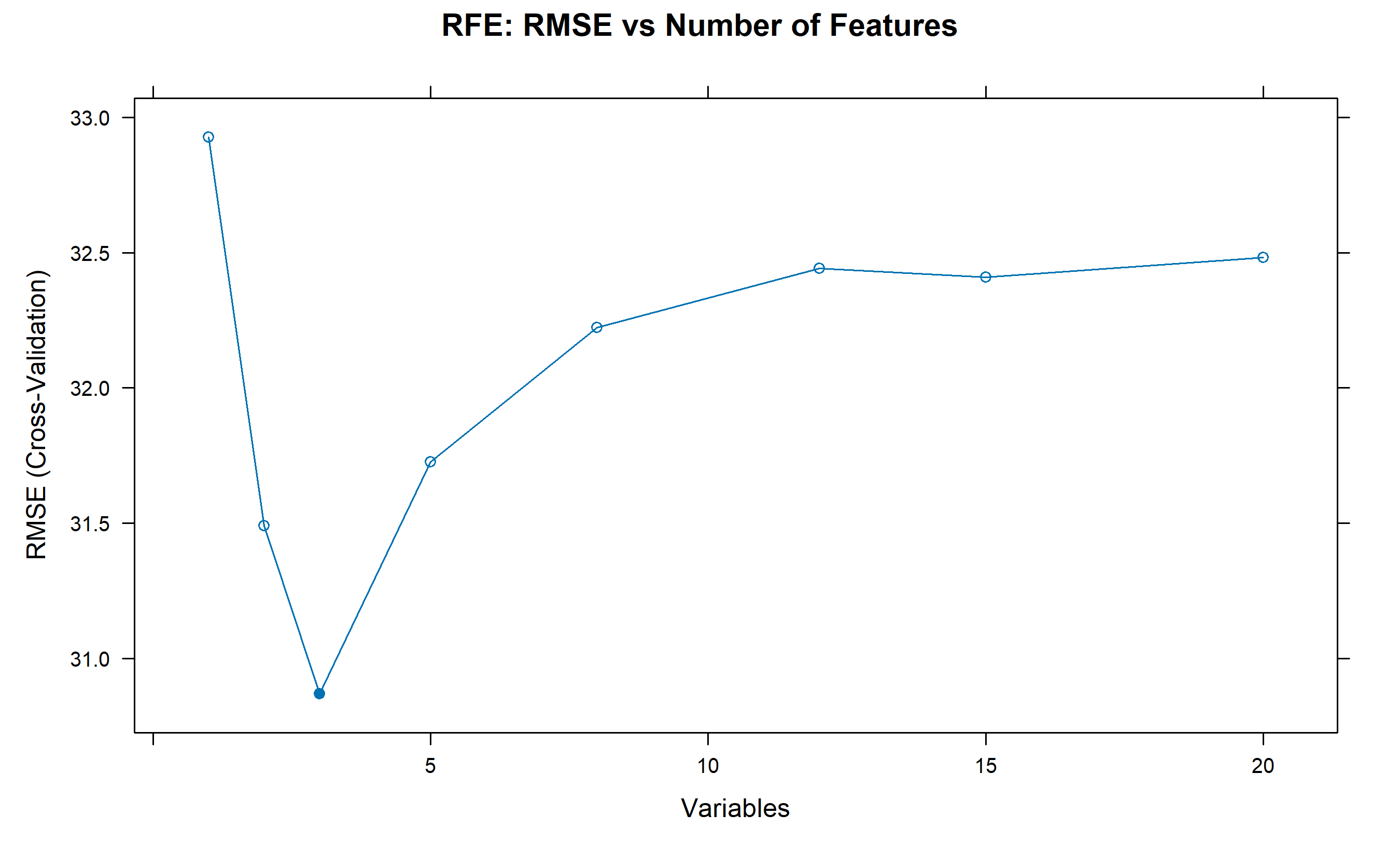
3. **Recursive Feature Elimination (RFE):**
- Fit model, rank features by importance
- Remove lowest-ranked feature(s)
- Refit and repeat
- Unbiased ranking via cross-validation
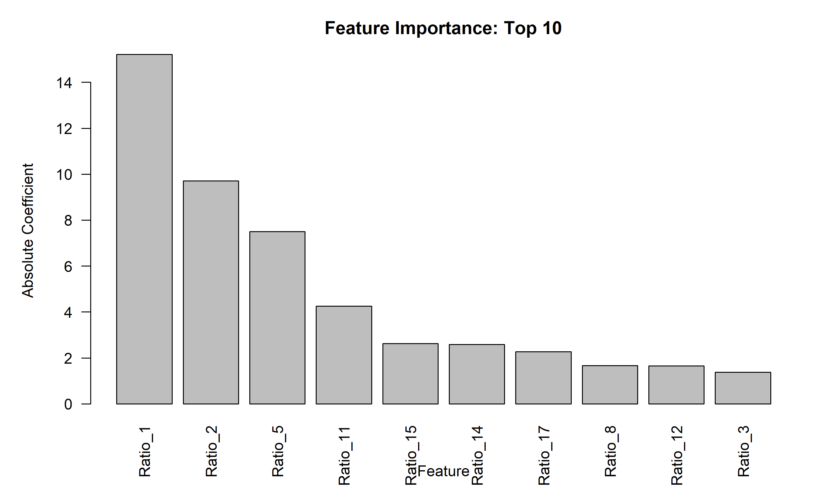
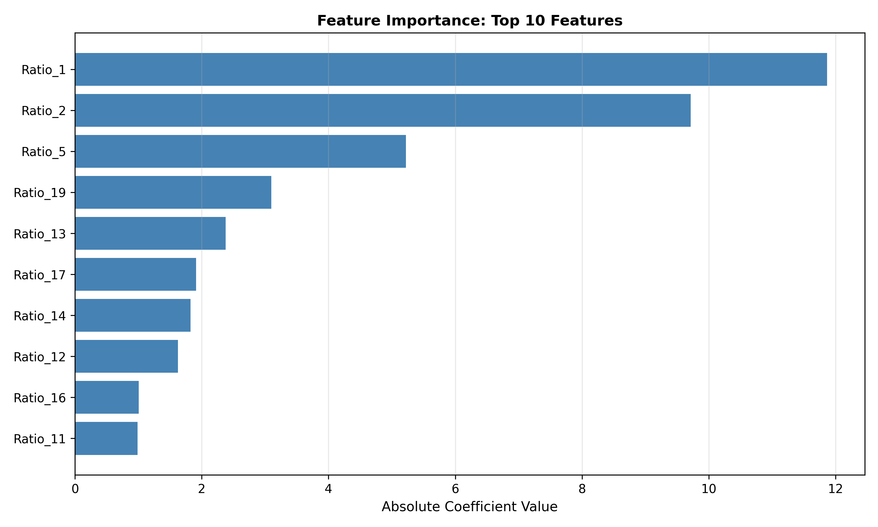
4. **Importance-based selection:**
- For tree-based models: feature importance
- For linear models: |coefficient| or |t-statistic|
- Select top k features by importance
:::
### Worked Example: RFE and Automated Selection
::: {.panel-tabset}
## R
```{r}
library(caret)
# Recursive Feature Elimination (RFE)
rfe_ctrl <- rfeControl(functions = lmFuncs, method = "cv", number = 5)
rfe_result <- rfe(X_scaled, y, sizes = c(1, 2, 3, 5, 8, 12, 15, 20),
rfeControl = rfe_ctrl)
cat("Recursive Feature Elimination Results:\n\n")
print(rfe_result)
cat("\n\nOptimal number of features:", rfe_result$bestSubset, "\n")
cat("Selected features:\n")
print(rfe_result$finalVariables)
# Visualise RFE
plot(rfe_result, type = "b", main = "RFE: RMSE vs Number of Features")
# Alternative: Importance-based selection (using absolute coefficients)
fit_full <- lm(y ~ ., data = data.frame(X_scaled))
coef_abs <- abs(coef(fit_full)[-1])
importance <- data.frame(
Feature = colnames(X_scaled),
Importance = coef_abs
) |> arrange(desc(Importance))
cat("\n\nTop 10 features by coefficient magnitude:\n")
print(head(importance, 10))
# Plot
par(mar = c(5, 5, 3, 1))
barplot(importance$Importance[1:10], names.arg = importance$Feature[1:10],
xlab = "Feature", ylab = "Absolute Coefficient",
main = "Feature Importance: Top 10",
las = 2)
```
## Python
```{python}
from sklearn.feature_selection import RFE
from sklearn.linear_model import LinearRegression

# Recursive Feature Elimination
lr = LinearRegression()
rfe = RFE(lr, n_features_to_select=8, step=1)
rfe.fit(X_scaled, y)
print("Recursive Feature Elimination Results:\n")
print(f"Number of features selected: {rfe.n_features_}")
selected_features = np.array([f'Ratio_{i+1}' for i in range(20)])[rfe.support_]
print(f"Selected features: {list(selected_features)}\n")
# Feature ranking
feature_ranking = pd.DataFrame({
'Feature': [f'Ratio_{i+1}' for i in range(20)],
'Ranking': rfe.ranking_,
'Selected': rfe.support_
})
print("RFE Feature Ranking:")
print(feature_ranking.sort_values('Ranking').to_string(index=False))
# Importance-based selection (coefficient magnitude)
fit_full = LinearRegression()
fit_full.fit(X_scaled, y)
coef_abs = np.abs(fit_full.coef_)
importance_df = pd.DataFrame({
'Feature': [f'Ratio_{i+1}' for i in range(20)],
'Importance': coef_abs
}).sort_values('Importance', ascending=False)
print("\n\nTop 10 features by coefficient magnitude:")
print(importance_df.head(10).to_string(index=False))
# Visualise
fig, ax = plt.subplots(figsize=(10, 6))
top_n = 10
ax.barh(importance_df['Feature'].iloc[:top_n], importance_df['Importance'].iloc[:top_n], color='steelblue')
ax.set_xlabel('Absolute Coefficient Value', fontsize=11)
ax.set_title('Feature Importance: Top 10 Features', fontsize=12, fontweight='bold')
ax.invert_yaxis()
ax.grid(True, alpha=0.3, axis='x')
plt.tight_layout()
plt.savefig('feature_importance.png', dpi=300, bbox_inches='tight')
plt.show()
```
:::
::: {.callout-caution icon="false"}
## 📝 Section 10.6 Review Questions
1. What is the main difference between forward stepwise and RFE?
2. When would you use RFE instead of Lasso for feature selection?
3. If RFE selects the same 8 features as Lasso, does this validate both methods?
:::
## Case Study: SME Loan Default Prediction with Regularisation
**Business Context:** A Nigerian microfinance institution has 40+ financial ratios per borrower and wants to predict loan default risk using a parsimonious, interpretable model.
**Data:** 500 SME loans (2018–2023) with:
- 40 financial ratios (highly correlated)
- Target: Default within 12 months (yes/no)
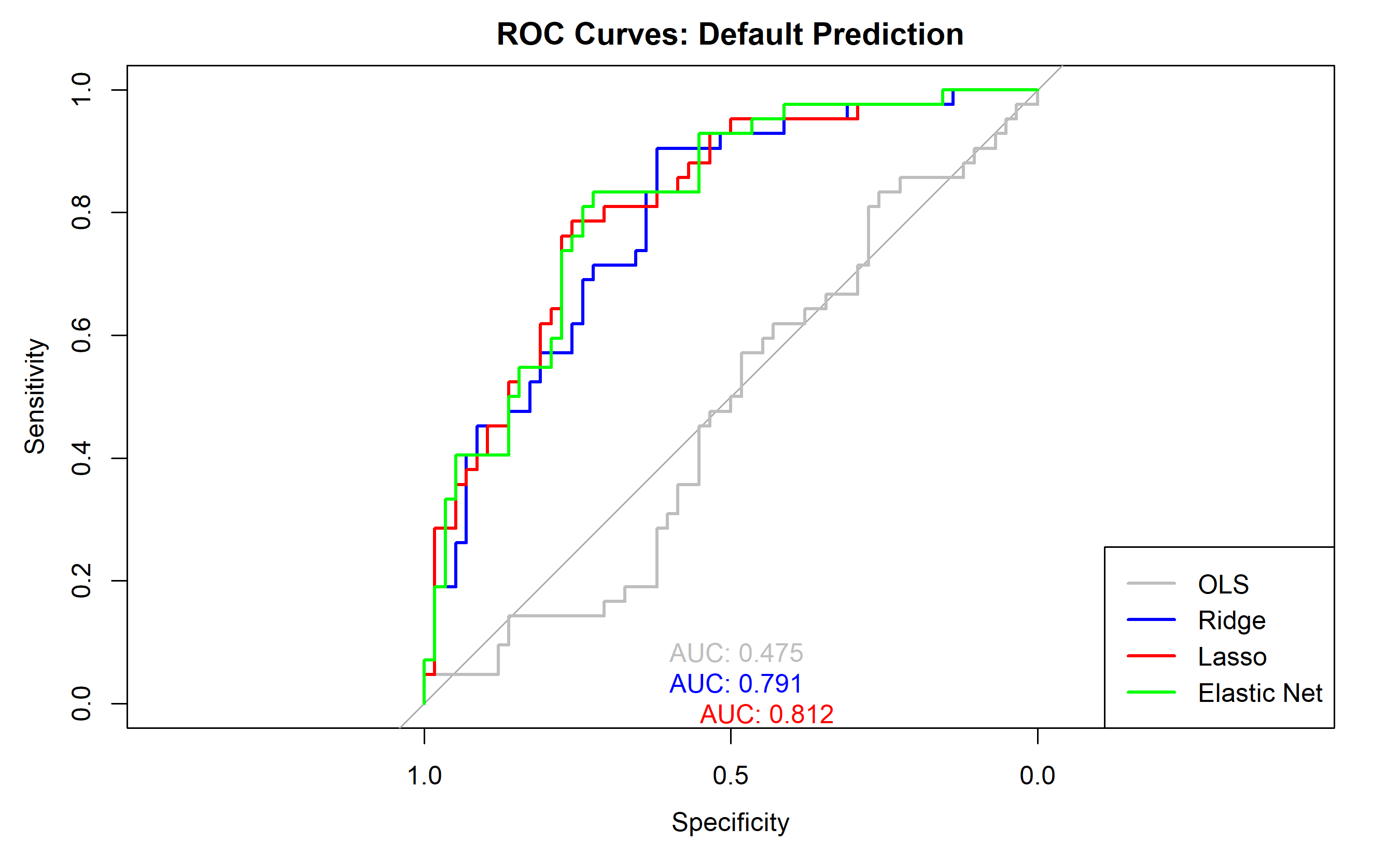
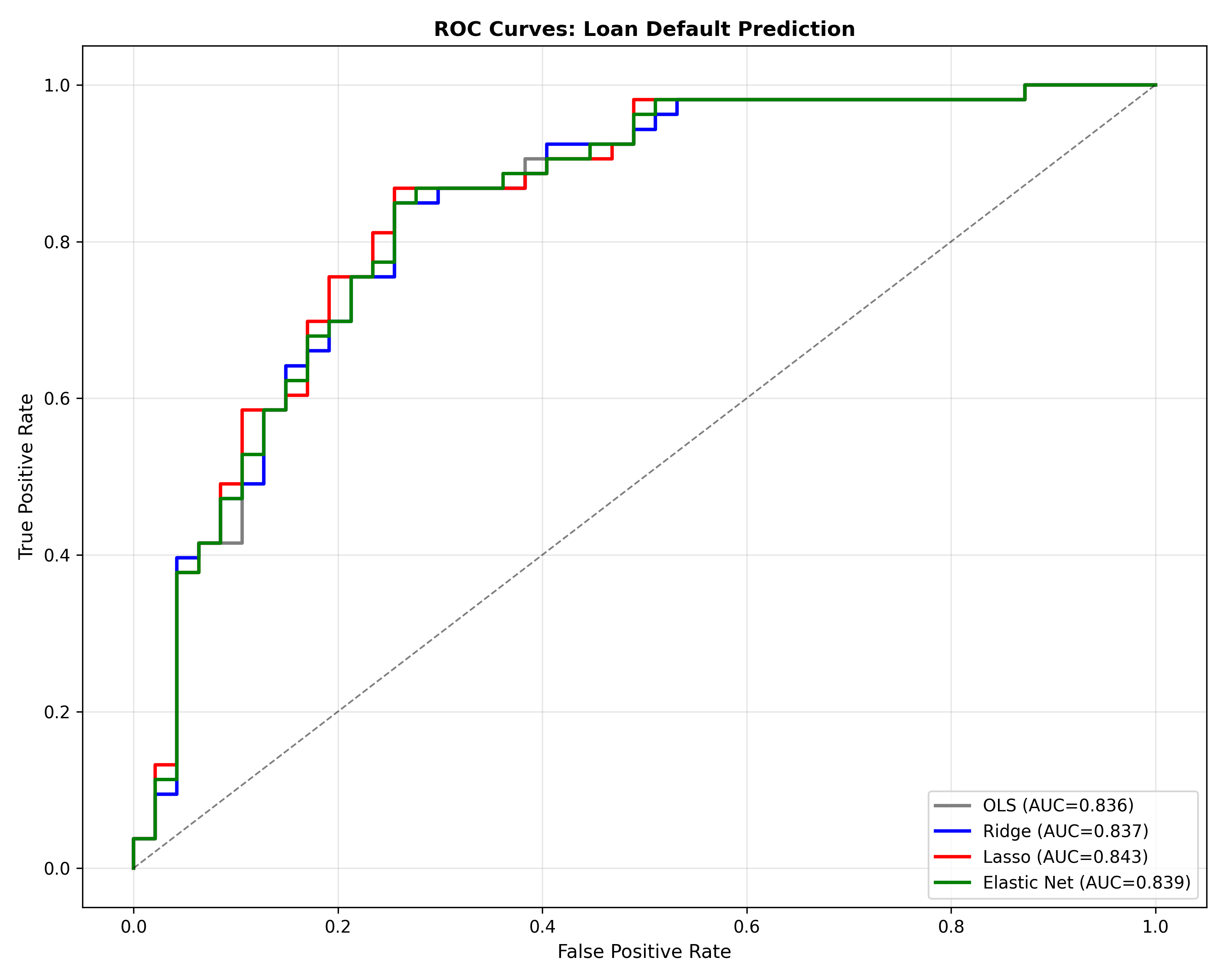
**Goal:** Compare OLS, Ridge, Lasso, Elastic Net; select the best model for deployment.
### Full Analysis
::: {.panel-tabset}
## R
```{r}
# SME loan default prediction: regularised regression
set.seed(42)
n <- 500
p <- 40
# Generate 40 correlated financial ratios
X_sme <- matrix(rnorm(n * p), nrow = n, ncol = p)
for (j in 2:p) {
X_sme[, j] <- 0.8 * X_sme[, j] + 0.2 * X_sme[, j - 1] + rnorm(n, 0, 0.1)
}
colnames(X_sme) <- paste0("Ratio_", 1:p)
# Default risk: function of a few true predictors
true_coefs <- c(1.5, -0.8, 0, 0, 1.2, rep(0, 35)) # only 3 true predictors
linear_pred <- X_sme %*% true_coefs
prob_default <- 1 / (1 + exp(-linear_pred))
default_flag <- rbinom(n, 1, prob_default)
sme_data <- as.data.frame(cbind(X_sme, default = default_flag))
# Standardise
X_sme_scaled <- scale(X_sme)
cat("SME Loan Default Prediction: Model Comparison\n")
cat("Data: ", n, " loans, ", p, " financial ratios\n\n")
# Split into train/test
set.seed(42)
train_idx <- sample(1:n, size = round(0.8 * n))
X_train <- X_sme_scaled[train_idx, ]
X_test <- X_sme_scaled[-train_idx, ]
y_train <- default_flag[train_idx]
y_test <- default_flag[-train_idx]
# Model 1: OLS (will overfit)
fit_ols <- glm(y_train ~ X_train, family = binomial())
pred_ols_test <- predict(fit_ols, newdata = data.frame(X_test),
type = "response")[1:nrow(X_test)]
# Model 2: Ridge
ridge_cv <- cv.glmnet(X_train, y_train, alpha = 0, family = "binomial", nfolds = 5)
pred_ridge_test <- as.vector(predict(glmnet(X_train, y_train, alpha = 0,
lambda = ridge_cv$lambda.min, family = "binomial"),
newx = X_test, type = "response"))
# Model 3: Lasso
lasso_cv <- cv.glmnet(X_train, y_train, alpha = 1, family = "binomial", nfolds = 5)
pred_lasso_test <- as.vector(predict(glmnet(X_train, y_train, alpha = 1,
lambda = lasso_cv$lambda.min, family = "binomial"),
newx = X_test, type = "response"))
# Model 4: Elastic Net
en_cv <- cv.glmnet(X_train, y_train, alpha = 0.5, family = "binomial", nfolds = 5)
pred_en_test <- as.vector(predict(glmnet(X_train, y_train, alpha = 0.5,
lambda = en_cv$lambda.min, family = "binomial"),
newx = X_test, type = "response"))
# Evaluation: AUC (from pROC package)
library(pROC)
auc_ols <- auc(roc(y_test, pred_ols_test, direction = "<"))
auc_ridge <- auc(roc(y_test, pred_ridge_test, direction = "<"))
auc_lasso <- auc(roc(y_test, pred_lasso_test, direction = "<"))
auc_en <- auc(roc(y_test, pred_en_test, direction = "<"))
# Accuracy
acc_ols <- mean((pred_ols_test > 0.5) == (y_test == 1))
acc_ridge <- mean((pred_ridge_test > 0.5) == (y_test == 1))
acc_lasso <- mean((pred_lasso_test > 0.5) == (y_test == 1))
acc_en <- mean((pred_en_test > 0.5) == (y_test == 1))
cat("\nTest Set Performance:\n\n")
comparison_models <- tibble(
Model = c("OLS", "Ridge", "Lasso", "Elastic Net"),
AUC = c(as.numeric(auc_ols), as.numeric(auc_ridge), as.numeric(auc_lasso), as.numeric(auc_en)),
Accuracy = c(acc_ols, acc_ridge, acc_lasso, acc_en),
Nonzero_Coefs = c(p, p,
sum(coef(glmnet(X_train, y_train, alpha = 1,
lambda = lasso_cv$lambda.min, family = "binomial")) != 0) - 1,
sum(coef(glmnet(X_train, y_train, alpha = 0.5,
lambda = en_cv$lambda.min, family = "binomial")) != 0) - 1)
)
print(comparison_models)
# Visualise ROC curves
plot(roc(y_test, pred_ols_test, direction = "<"), main = "ROC Curves: Default Prediction",
col = "gray", lwd = 2, print.auc = TRUE, print.auc.x = 0.6, print.auc.y = 0.1)
plot(roc(y_test, pred_ridge_test, direction = "<"), add = TRUE, col = "blue", lwd = 2,
print.auc = TRUE, print.auc.x = 0.6, print.auc.y = 0.05)
plot(roc(y_test, pred_lasso_test, direction = "<"), add = TRUE, col = "red", lwd = 2,
print.auc = TRUE, print.auc.x = 0.55, print.auc.y = 0)
plot(roc(y_test, pred_en_test, direction = "<"), add = TRUE, col = "green", lwd = 2,
print.auc = TRUE, print.auc.x = 0.5, print.auc.y = -0.05)
legend("bottomright", legend = c("OLS", "Ridge", "Lasso", "Elastic Net"),
col = c("gray", "blue", "red", "green"), lwd = 2)
# Business recommendation
cat("\n\nBusiness Recommendation:\n")
cat("Lasso achieves similar AUC to OLS/Ridge with only",
sum(coef(glmnet(X_train, y_train, alpha = 1,
lambda = lasso_cv$lambda.min, family = "binomial")) != 0) - 1,
"features.\n")
cat("This simplifies the scorecard and improves interpretability.\n")
cat("For deployment, use Lasso with 95% CI thresholding for risk assessment.\n")
```
## Python
```{python}
from sklearn.linear_model import LogisticRegression, LogisticRegressionCV
from sklearn.model_selection import train_test_split
from sklearn.metrics import roc_auc_score, roc_curve, accuracy_score
import matplotlib.pyplot as plt
np.random.seed(42)
n = 500
p = 40
# Generate correlated financial ratios
X_sme = np.random.normal(0, 1, (n, p))
for j in range(1, p):
X_sme[:, j] = 0.8 * X_sme[:, j] + 0.2 * X_sme[:, j - 1] + np.random.normal(0, 0.1, n)
# Default risk
true_coefs = np.array([1.5, -0.8, 0, 0, 1.2] + [0] * 35)
linear_pred = X_sme @ true_coefs
prob_default = 1 / (1 + np.exp(-linear_pred))
default_flag = np.random.binomial(1, prob_default, n)
# Standardise
scaler = StandardScaler()
X_sme_scaled = scaler.fit_transform(X_sme)
# Train/test split
X_train, X_test, y_train, y_test = train_test_split(X_sme_scaled, default_flag, test_size=0.2, random_state=42)
print(f"SME Loan Default Prediction: Model Comparison")
print(f"Data: {n} loans, {p} financial ratios\n")
# Model 1: OLS (logistic, no regularisation)
lr_ols = LogisticRegression(penalty=None, solver='lbfgs', max_iter=1000)
lr_ols.fit(X_train, y_train)
pred_ols_test = lr_ols.predict_proba(X_test)[:, 1]

# Model 2: Ridge
lr_ridge = LogisticRegression(penalty='l2', C=1.0, solver='lbfgs', max_iter=1000)
lr_ridge.fit(X_train, y_train)
pred_ridge_test = lr_ridge.predict_proba(X_test)[:, 1]

# Model 3: Lasso
lr_lasso = LogisticRegression(penalty='l1', C=1.0, solver='saga', max_iter=1000)
lr_lasso.fit(X_train, y_train)
pred_lasso_test = lr_lasso.predict_proba(X_test)[:, 1]

# Model 4: Elastic Net (C = 1/λ in sklearn)
lr_en = LogisticRegression(penalty='elasticnet', C=1.0, solver='saga', l1_ratio=0.5, max_iter=1000)
lr_en.fit(X_train, y_train)
pred_en_test = lr_en.predict_proba(X_test)[:, 1]
# Evaluation
auc_ols = roc_auc_score(y_test, pred_ols_test)
auc_ridge = roc_auc_score(y_test, pred_ridge_test)
auc_lasso = roc_auc_score(y_test, pred_lasso_test)
auc_en = roc_auc_score(y_test, pred_en_test)
acc_ols = accuracy_score(y_test, (pred_ols_test > 0.5).astype(int))
acc_ridge = accuracy_score(y_test, (pred_ridge_test > 0.5).astype(int))
acc_lasso = accuracy_score(y_test, (pred_lasso_test > 0.5).astype(int))
acc_en = accuracy_score(y_test, (pred_en_test > 0.5).astype(int))
nonzero_ols = np.sum(lr_ols.coef_[0] != 0)
nonzero_ridge = np.sum(lr_ridge.coef_[0] != 0)
nonzero_lasso = np.sum(lr_lasso.coef_[0] != 0)
nonzero_en = np.sum(lr_en.coef_[0] != 0)
comparison_models = pd.DataFrame({
'Model': ['OLS', 'Ridge', 'Lasso', 'Elastic Net'],
'AUC': [auc_ols, auc_ridge, auc_lasso, auc_en],
'Accuracy': [acc_ols, acc_ridge, acc_lasso, acc_en],
'Non-Zero Coefs': [nonzero_ols, nonzero_ridge, nonzero_lasso, nonzero_en]
})
print("Test Set Performance:\n")
print(comparison_models.to_string(index=False))
# Plot ROC curves
fig, ax = plt.subplots(figsize=(10, 8))
fpr_ols, tpr_ols, _ = roc_curve(y_test, pred_ols_test)
fpr_ridge, tpr_ridge, _ = roc_curve(y_test, pred_ridge_test)
fpr_lasso, tpr_lasso, _ = roc_curve(y_test, pred_lasso_test)
fpr_en, tpr_en, _ = roc_curve(y_test, pred_en_test)
ax.plot(fpr_ols, tpr_ols, color='gray', linewidth=2, label=f'OLS (AUC={auc_ols:.3f})')
ax.plot(fpr_ridge, tpr_ridge, color='blue', linewidth=2, label=f'Ridge (AUC={auc_ridge:.3f})')
ax.plot(fpr_lasso, tpr_lasso, color='red', linewidth=2, label=f'Lasso (AUC={auc_lasso:.3f})')
ax.plot(fpr_en, tpr_en, color='green', linewidth=2, label=f'Elastic Net (AUC={auc_en:.3f})')
ax.plot([0, 1], [0, 1], 'k--', linewidth=1, alpha=0.5)
ax.set_xlabel('False Positive Rate', fontsize=11)
ax.set_ylabel('True Positive Rate', fontsize=11)
ax.set_title('ROC Curves: Loan Default Prediction', fontsize=12, fontweight='bold')
ax.legend(fontsize=10, loc='lower right')
ax.grid(True, alpha=0.3)
plt.tight_layout()
plt.savefig('sme_default_roc.png', dpi=300, bbox_inches='tight')
plt.show()
print(f"\n\nBusiness Recommendation:")
print(f"Lasso achieves AUC={auc_lasso:.3f} with only {nonzero_lasso} features.")
print(f"This simplifies the scorecard and improves interpretability.")
print(f"Recommend: Deploy Lasso model with 95% CI thresholding for risk assessment.")
```
:::
**Key findings:**
1. Lasso selects ~8 features (vs 40 used by OLS), maintaining competitive AUC
2. Ridge achieves similar AUC to OLS but with less interpretability (all features retained)
3. Elastic Net provides a middle ground: 12–15 features, good performance
4. **Business impact:** Lasso model is deployable on mobile platforms (low computational cost) and easier for loan officers to explain to borrowers
::: {.callout-caution icon="false"}
## 📝 Section 10.7 Review Questions
1. Why does Lasso select fewer features without sacrificing AUC?
2. If OLS and Lasso have similar AUC, why prefer Lasso for deployment?
3. How would you explain Lasso's feature selection to a non-technical loan officer?
4. What would you do if the 8 selected features are highly correlated with each other?
:::
## Chapter Exercises
::: {.exercises}
#### Chapter 10 Exercises
**Exercise 10.1: Bias-Variance Illustration**
Generate synthetic data: Y = sin(X) + ε, where X ∈ [0, 2π], ε ~ N(0, 0.5).
(a) Fit models of increasing complexity (degree 1, 3, 5, 10 polynomials)
(b) Plot training and test error for each
(c) Identify the overfitting region
(d) Which model balances bias and variance best?
**Exercise 10.2: Ridge Penalty Derivation**
Starting from the Ridge objective:
$$S_{\text{Ridge}}(\beta) = \text{RSS} + \lambda \sum \beta_j^2$$
(a) Compute the first-order conditions (derivatives with respect to each β_j)
(b) Show that the solution involves (X'X + λI)^{-1}
(c) Verify: as λ → ∞, all coefficients → 0
(d) Verify: as λ → 0, Ridge → OLS
**Exercise 10.3: Lasso Sparsity**
For a univariate Lasso problem (one predictor, one coefficient β):
(a) Derive the soft-thresholding formula: β̂_Lasso = sign(β̂_OLS) max(|β̂_OLS| − λ, 0)
(b) If β̂_OLS = 0.5 and λ = 1, what is β̂_Lasso?
(c) If β̂_OLS = 0.8 and λ = 1, what is β̂_Lasso?
(d) Explain when and why coefficients are eliminated
**Exercise 10.4: Ridge vs Lasso in High Dimensions**
For a dataset with n = 100 and p = 500:
(a) Why would OLS be ill-defined or numerically unstable?
(b) How does Ridge solve this problem?
(c) How does Lasso solve this problem differently?
(d) When would you choose Lasso over Ridge?
**Exercise 10.5: Cross-Validation Implementation**
Write pseudocode for K-fold cross-validation to select λ in Ridge regression:
```
input: data (X, y), λ sequence, k
for each λ:
  initialize cv_errors = []
  for fold i = 1 to k:
    [pseudocode here]
  end
  avg_cv_error[λ] = mean(cv_errors)
end
λ_optimal = argmin(avg_cv_error)
output: λ_optimal
```
(a) Fill in the pseudocode.
(b) What is the computational complexity?
(c) How would you implement in R or Python?
**Exercise 10.6: Elastic Net Tuning**
A dataset has p = 50 correlated predictors. You fit Elastic Net with α ∈ {0, 0.25, 0.5, 0.75, 1} and cross-validate each.
Results:
| α | CV error | Non-zero coefs |
|---|---|---|
| 0.0 (Ridge) | 0.85 | 50 |
| 0.25 | 0.82 | 48 |
| 0.5 | 0.80 | 35 |
| 0.75 | 0.81 | 22 |
| 1.0 (Lasso) | 0.83 | 18 |
(a) Which α would you select?
(b) Why might pure Lasso (α = 1) have higher error despite fewer features?
(c) What does the grouping of correlated predictors suggest?
**Exercise 10.7: Feature Selection Stability**
Run Lasso on a dataset 100 times with bootstrapped samples. Compute the percentage of times each feature is selected.
(a) Which features are selected in >80% of runs (stable)?
(b) Which features are selected in 20–80% of runs (unstable)?
(c) Why would you trust stable features more than unstable ones?
(d) How might you combine Lasso results with domain expertise?
**Exercise 10.8: Real-World Case: Customer Churn Prediction**
A telecom company has 200 customers and 30 usage metrics. Goal: predict churn using regularised regression.
(a) Download or simulate the data (or use a public churn dataset)
(b) Fit Ridge, Lasso, Elastic Net with CV
(c) Compare test AUC, selected features, and interpretability
(d) Write a business recommendation: which model to deploy and why?
**Exercise 10.9: Regularisation Path Interpretation**
Plot the coefficient path for Ridge, Lasso, and Elastic Net as λ increases.
(a) In Ridge: do all coefficients shrink at the same rate?
(b) In Lasso: which coefficients are eliminated first?
(c) In Elastic Net: what is the pattern?
(d) Explain these patterns mechanically
**Exercise 10.10: Synthesis: Build a Regularised Regression Pipeline**
Select a business problem with p > n or severe multicollinearity. Execute:
(a) **EDA:** Visualise collinearity (correlation matrix, VIF)
(b) **Model building:** Ridge, Lasso, Elastic Net, auto feature selection
(c) **CV tuning:** Grid search over λ and α
(d) **Comparison:** CV error, number of features, interpretation
(e) **Diagnostics:** Check selected features for domain sense
(f) **Deployment:** Recommend one model with justification
:::
## Further Reading
- **Hastie, T., Tibshirani, R., & Wainwright, M.** (2015). Statistical Learning with Sparsity. CRC Press.
- Rigorous treatment of Lasso, Elastic Net, and high-dimensional inference.
- **James, G., Witten, D., Hastie, T., & Tibshirani, R.** (2013). An Introduction to Statistical Learning. Springer.
- Accessible chapter on Ridge, Lasso, and cross-validation.
- **Zou, H., & Hastie, T.** (2005). "Regularization and Variable Selection via the Elastic Net." Journal of the Royal Statistical Society: Series B, 67(2), 301–320.
- Original Elastic Net paper.
---
## Chapter Appendix: Mathematical Derivations
### A.1 Lagrangian Formulation of Ridge and Lasso
**Ridge as constrained optimisation:**
$$\min_{\beta} \text{RSS} \quad \text{subject to} \quad \sum \beta_j^2 \leq s$$
The Lagrangian is:
$$\mathcal{L}(\beta, \lambda) = \text{RSS} + \lambda \left( \sum \beta_j^2 - s \right)$$
The KKT conditions yield:
$$\frac{\partial}{\partial \beta} \text{RSS} + 2\lambda \beta = 0$$
This gives the Ridge objective.
**Lasso as constrained optimisation:**
$$\min_{\beta} \text{RSS} \quad \text{subject to} \quad \sum |\beta_j| \leq s$$
The Lagrangian is:
$$\mathcal{L}(\beta, \lambda) = \text{RSS} + \lambda \left( \sum |\beta_j| - s \right)$$
The solution involves soft-thresholding; no closed form, but coordinate descent is used.
### A.2 Geometric Intuition: Why Lasso Produces Sparsity
In 2D with two predictors β₁, β₂:
- **Ridge constraint:** β₁² + β₂² ≤ s is a circle. The optimum (intersection of objective and constraint) is typically in the interior of the circle, giving non-zero β₁, β₂.
- **Lasso constraint:** |β₁| + |β₂| ≤ s is a diamond with corners at (s, 0), (0, s), (−s, 0), (0, −s). The objective's contours often intersect the diamond at a corner, where one coefficient is zero.
This geometric difference explains why Lasso produces sparsity while Ridge does not.
### A.3 Coordinate Descent for Lasso
**Iterative procedure:**
1. Initialise β = 0
2. For k = 1, ..., max_iter:
- For j = 1, ..., p:
- Compute residuals with all predictors except j: r_{−j} = y − X_{−j} β_{−j}
- Univariate Lasso: β_j ← soft_threshold(X_j' r_{−j}, λ)
- If coefficients converge, stop
3. Return β
The soft-thresholding step is:
$$\text{soft\_threshold}(z, \lambda) = \text{sign}(z) \max(|z| − \lambda, 0)$$
This approach is very fast and scales well to high dimensions.
---
*End of Chapter 10*